Performance of Fine-Tuning Convolutional Neural Networks for HEp-2 Image Classification - MDPI
←
→
Page content transcription
If your browser does not render page correctly, please read the page content below
applied
           sciences
Technical Note
Performance of Fine-Tuning Convolutional Neural
Networks for HEp-2 Image Classification
Vincenzo Taormina 1 , Donato Cascio 2, * , Leonardo Abbene 2 and Giuseppe Raso 2
 1    Department of Engineering, University of Palermo, 90128 Palermo, Italy; vincenzo.taormina@unipa.it
 2    Department of Physics and Chemistry, University of Palermo, 90128 Palermo, Italy;
      leonardo.abbene@unipa.it (L.A.); giuseppe.raso@unipa.it (G.R.)
 *    Correspondence: donato.cascio@unipa.it

 Received: 8 September 2020; Accepted: 1 October 2020; Published: 3 October 2020

 Abstract: The search for anti-nucleus antibodies (ANA) represents a fundamental step in the
 diagnosis of autoimmune diseases. The test considered the gold standard for ANA research is indirect
 immunofluorescence (IIF). The best substrate for ANA detection is provided by Human Epithelial type
 2 (HEp-2) cells. The first phase of HEp-2 type image analysis involves the classification of fluorescence
 intensity in the positive/negative classes. However, the analysis of IIF images is difficult to perform
 and particularly dependent on the experience of the immunologist. For this reason, the interest of
 the scientific community in finding relevant technological solutions to the problem has been high.
 Deep learning, and in particular the Convolutional Neural Networks (CNNs), have demonstrated
 their effectiveness in the classification of biomedical images. In this work the efficacy of the CNN
 fine-tuning method applied to the problem of classification of fluorescence intensity in HEp-2 images
 was investigated. For this purpose, four of the best known pre-trained networks were analyzed
 (AlexNet, SqueezeNet, ResNet18, GoogLeNet). The classifying power of CNN was investigated with
 different training modalities; three levels of freezing weights and scratch. Performance analysis was
 conducted, in terms of area under the ROC (Receiver Operating Characteristic) curve (AUC) and
 accuracy, using a public database. The best result achieved an AUC equal to 98.6% and an accuracy of
 93.9%, demonstrating an excellent ability to discriminate between the positive/negative fluorescence
 classes. For an effective performance comparison, the fine-tuning mode was compared to those in
 which CNNs are used as feature extractors, and the best configuration found was compared with
 other state-of-the-art works.

 Keywords: CNNs; autoimmune diseases; IIF test; HEp-2; deep learning; fine-tuning;
 features extractors

1. Introduction
     Autoimmune diseases occur whenever the immune system is activated in an abnormal way and
attacks healthy cells, instead of defending them from pathogens; thus, causing functional or anatomical
alterations of the affected district. [1]. There are at least 80 types of known autoimmune diseases
(AD) [1]. AD can affect almost any part of the body i.e., tissue, organ, body system [2]. The anti-nucleus
autoantibodies (ANA) are directed towards distinct components of the nucleus and are traditionally
sought after with the indirect immunofluorescence (IIF) technique. With this method, in addition to
the antibodies directed towards nuclear components, antibodies directed towards antigens are also
highlighted and located in other cellular compartments. When Human Epithelial type 2 (HEp-2) cells
are used as a substrate, the IIF method allows the detection of autoantibodies to at least 30 distinct
nuclear and cytoplasmic antigens [3]. For this reason, the IIF technique with HEp-2 substrate is

Appl. Sci. 2020, 10, 6940; doi:10.3390/app10196940                                 www.mdpi.com/journal/applsci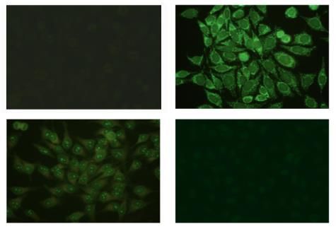
patterns with which fluorescence can occur are associated with groups of autoimmune diseases.
      In the IIF image analysis flow, the first phase concerns the fluorescence intensity classification.
This phase is obviously of considerable importance in the diagnostic workflow, as it aims to
discriminate on the presence/absence of autoimmune diseases. Figure 1 shows examples of
positive/negative class.
Appl. Sci. 2020, 10, 6940                                                                                           2 of 20
      However, the analysis of IIF images, as a whole, and in particular, in regards to the analysis of
intensity, is extremely complex and linked to the experience of the immunologist [4]. For this reason,
in recent years
considered     the goldtherestandard
                              have been
                                      test numerous      scientific
                                           for the diagnosis        works aimeddiseases.
                                                                of autoimmune         at obtaining   automatic
                                                                                              The patterns   withsupport
                                                                                                                   which
systems for HEp-2
fluorescence      can occurimage
                               are analysis
                                   associated[5,6].
                                                withIngroups
                                                        particular, in the last few
                                                                of autoimmune          years, various research groups
                                                                                    diseases.
interested
      In the inIIF the
                    image topic  have flow,
                              analysis  tried the
                                               to first
                                                    exploit  theconcerns
                                                         phase     potentialtheoffered   by recent
                                                                                 fluorescence         machine
                                                                                               intensity        learning
                                                                                                           classification.
techniques
This  phase isinobviously
                   order to address     the problem
                               of considerable          of the in
                                                importance     classification
                                                                  the diagnosticof HEp-2   images.
                                                                                    workflow,       However,
                                                                                              as it aims        the topic
                                                                                                         to discriminate
of fluorescence
on                    intensity of
    the presence/absence         classification
                                    autoimmune   is diseases.
                                                    still poorly  addressed
                                                               Figure  1 shows [7].examples of positive/negative class.

     Figure 1. Examples of indirect immunofluorescence (IIF) images with different fluorescence intensity:
     Figure 1. Examples of indirect immunofluorescence (IIF) images with different fluorescence intensity:
     in the upper left a positive centrioles image, in the upper right a positive cytoplasmic image, in the
     in the upper left a positive centrioles image, in the upper right a positive cytoplasmic image, in the
     lower left a positive nucleolar image, in the lower right a negative image. The positivity/negativity
     lower left a positive nucleolar image, in the lower right a negative image. The positivity/negativity of
     of fluorescence is not strictly correlated with the luminous intensity of the Human Epithelial type 2
     fluorescence is not strictly correlated with the luminous intensity of the Human Epithelial type 2
     (HEp-2) images; the image in the upper left for example, although presenting low light intensity, has a
     (HEp-2) images; the image in the upper left for example, although presenting low light intensity, has
     positive fluorescence intensity.
     a positive fluorescence intensity.
     However, the analysis of IIF images, as a whole, and in particular, in regards to the analysis
      Over the past decade, the popularity of methods that exploit deep learning techniques has
of intensity, is extremely complex and linked to the experience of the immunologist [4]. For this
considerably increased, evidently as deep learning has improved the state-of-the-art methods in
reason, in recent years there have been numerous scientific works aimed at obtaining automatic
research fields, such as speech recognition and computer vision [8]. Although neural networks had
support systems for HEp-2 image analysis [5,6]. In particular, in the last few years, various research
their scientific boom already in the 80s, their recent success can be attributed to an increased
groups interested in the topic have tried to exploit the potential offered by recent machine learning
availability of data, improvements in hardware/software [9], and new algorithms capable of both
techniques in order to address the problem of the classification of HEp-2 images. However, the topic of
speeding up learning in the training phase and improving the generalization of new data [10].
fluorescence intensity classification is still poorly addressed [7].
      In the field of computer vision, deep learning has expressed its potential in image processing
     Over the past decade, the popularity of methods that exploit deep learning techniques has
thanks to Convolutional Neural Networks (CNNs). In recent years there have been several fields of
considerably increased, evidently as deep learning has improved the state-of-the-art methods in
use of CNNs that, nowadays, allow the development of important applications. Some examples are:
research fields, such as speech recognition and computer vision [8]. Although neural networks had
the antispoofing of the face and iris [11], recognition of highway traffic congestion [12], the image
their scientific boom already in the 80s, their recent success can be attributed to an increased availability
steganography and steganalysis [13], the galaxy morphology classification [14], drone detection, and
of data, improvements in hardware/software [9], and new algorithms capable of both speeding up
classification [15,16].
learning in the training phase and improving the generalization of new data [10].
     In the field of computer vision, deep learning has expressed its potential in image processing
thanks to Convolutional Neural Networks (CNNs). In recent years there have been several fields of
use of CNNs that, nowadays, allow the development of important applications. Some examples are:
the antispoofing of the face and iris [11], recognition of highway traffic congestion [12], the image
steganography and steganalysis [13], the galaxy morphology classification [14], drone detection,
and classification [15,16].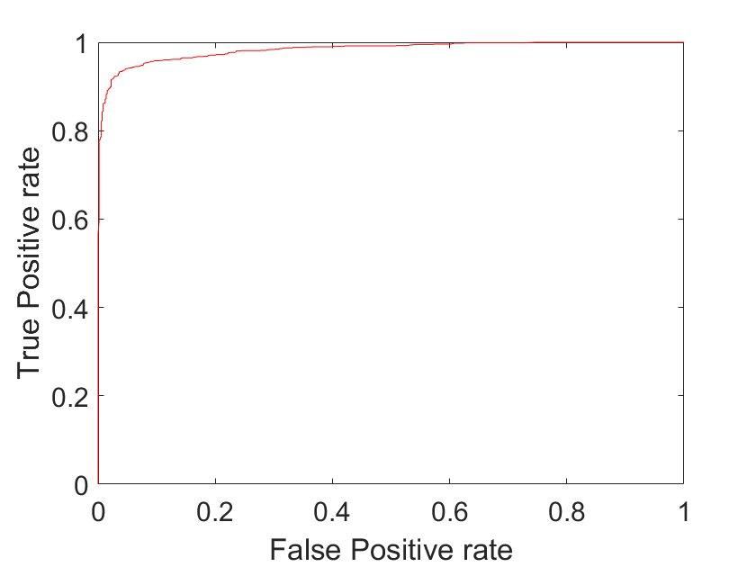
Appl. Sci. 2020, 10, 6940                                                                            3 of 20

     Conceptually, the CNNs are inspired by the visual system as proposed in the works of Hubel
and Wiesel on cat and monkey visual cortices [17]. A CNN accepts an image directly as input and
applies a hierarchy of different convolution kernels to it. The first layers allow extraction of elementary
visual features, such as oriented edges, end-points, and corners, and are gradually combined with
subsequent layers in order to detect higher-order features [18].
     In the field of image classification in general, CNNs can be used, proposing ad-hoc architecture
and proceeding with its training, or using pre-trained architecture. In the latter case, the training on
specific data to the problem can be carried out from scratch, or through fine-tuning of a part of the
parameters/weights of the pre-trained network.
     Fine-tuning is known as transfer learning, as the knowledge of another problem is exploited to
solve the object of the study. Furthermore, a pre-trained CNN architecture can be modified in its
architecture before carrying out training or fine-tuning.
     In our previous work [19], we started to tackle the problem of fluorescence intensity classification
by means of CNNs, but we did it by limiting their use to feature extractors. In this study, we analyzed
various known CNNs and their respective layers from which to extract the features that allowed
classification by means of Support Vector Machine (SVM) classifiers. The advantage of this type of work
is the simplicity of implementation (no retraining of the pre-trained networks must be carried out),
the disadvantage is usually relatively lower performances than those obtained from the pre-trained
networks with the fine-tuning method. This is confirmed in the recent review by Rahman et al. [7],
in fact the authors, regarding our previous work, comment as follows: “It is believed that the adoption
of features from a fine-tuned CNN model would further improve the performance of Cascio et al.
(2019c)’s method “.
     The importance of the topic, the fact that it has been little addressed by the scientific community,
and the possibility of analyzing the effectiveness of pre-trained networks, training them with the
performing mode of fine-tuning, were the motivations that led us to face the problem of fluorescence
intensity classification in HEp-2 images.

2. Literature Review
      Numerous contributions have been made in recent years by the scientific community in the
classification of HEp-2 images, especially due to contests organized on the subject, such as ICPR
2012 [20], ICIP 2013 [21], and ICPR 2014 [22]. However, these competitions have only dealt with the
theme of pattern classification, considering 6/7 classes of significant interest.
      In Li and Shen’s work [23], a deep cross residual network (DCR-Net) was proposed. The structure
is similar to DenseNet, but the authors, in order to minimize the vanishing gradient problem, added
cross-residual shortcuts between some layers to the original network. The advantage of the change is to
increase the depth of the network by improving feature representation. They made a date augmentation
for rotations. The database used is I3A Task 1 and MIVIA. The method showed a Mean Class Accuracy
(MCA) of 85,1% on a private test of I3A database.
      Manivannan et al. [24] proposed a method that allowed them to win the ICPR 2014 contest with an
MCA of 87.1%. They extracted a local feature vector that is aggregated via sparse coding. The method
uses a pyramidal decomposition of the cell analyzed in the central part and in the crown that contains
the cell membrane. Linear SVMs are the classifiers used on the learned dictionary. Specifically, they use
four SVMs, the first one trained on the orientation of the original images, and the remaining three,
respectively, on the images rotated by 90/180/270 degrees.
      In a few cases, the authors have ventured into unsupervised classifications methods for the
analysis of HEp-2 images [25,26]. In these cases, the number of analyzed patterns was reduced.
In [25], the authors compared the method called BoW (Bag of Words), based on hand-crafted features
and the deep learning model as learning hierarchical features, by clustering unsupervised learning.
The authors obtained the best results with the BoW model. They demonstrated that, while the deep
learning model allows better extraction of global features, the BoW model is better at extracting local
Appl. Sci. 2020, 10, 6940 4 of 20
features. In [26], the authors proposed the grouping of centromeres present on the cells through a
clustering K-means algorithm; the method allows the identification and classification of the centromere
pattern. The method is tested on two public databases, MIVIA and Auto-Immunité, Diagnostic Assisté
par ordinateur (AIDA), on which accuracy performances of 92% and 98%, respectively, are obtained.
Despite the high indexing performance of the centromeric pattern, being able to classify only one type
of pattern is certainly a limitation for the method.
Only recently has deep learning been applied to the various fields of HEp-2 image analysis [7].
In this context, one of the first works on the classification of HEp-2 images in which CNN was used
is due to Gao et al. [27]. In this work, a CNN having eight layers, compared to the Bag of Features
and Fisher Vector methods, was compared. The proposed CNN architecture has six convolution-type
layers with pooling operations, and two fully-connected layers. The database used for the test is I3A
Task 1 and MIVIA. The authors obtained 96.76% of mean class accuracy (MCA) and 97.24% of accuracy.
In [28], the authors used well-known CNNs in the pre-trained mode as vector feature extractors
and trained multiple SVM classifiers in the one-against-all (OAA) mode. This strategy is one of the best
known for breaking down a multi-class problem into a series of binary classifiers. Instead of using the
classic OAA scheme, in which the test is assigned to the majority classifier result, the authors proposed
the use of a K-nearest neighbors (KNN) based classifier as a collector of the various ensemble results.
The performances on the public database I3A are in terms of MCA 82.16% and 93.75% at the cell level,
and at the image level, respectively.
Some research groups have dealt with other aspects in the field of HEp-2 images, such as
segmentation [29] and the search for mitosis [30].
The problem of classifying the intensity of fluorescence has certainly been little addressed [7].
The reason is probably due to the lack of public databases containing both positive and negative images;
to date, it seems that the only public database of HEp-2 images with these characteristics is AIDA [4].
In Merone et al. [31], the problem of fluorescence intensity analysis was addressed but the authors
did not make a classification between positive and negative, rather between positive, negative and
weak positive. The authors extracted features through an Invariant Scattering Convolutional Network
and used SVM classifiers with a Gaussian kernel. The network was based on multiple wavelet module
operators and was used as a texture description. To classify the tree-class the authors applied the
one-on-one approach and trained the tree binary classifier (negative vs. positive/negative vs. weak
positive/negative vs. weak positive). Their method was trained on a private database of 570 wells
for a total of 1771 images in which the fluorescence intensity was blindly classified by two doctors.
The accuracy reported in the private database was 89.5%.
A classification of fluorescence intensity into positive vs. weak positive was also carried out by
Di Cataldo et al. [32]. The authors used local contrast features at multiple scales and a KNN classifier
to characterize the image, thereby achieving an accuracy of 85% in fluorescent intensity discrimination.
In Bennamar Elgaaied et al. [4] the authors have implemented a method based on SVM to classify
the HEp-2 images in positive or negative intensity. They achieved an accuracy of 85.5% using traditional
features based on intensity, geometry, and shape. The same set of tests was analyzed by two young
immunologists verifying a greater ability of the automatic system (85.5% vs. 66%).
Other authors addressed the classification in positive/negative intensity on private databases.
Iannello et al. [33] used a private database with 914 images to train a classifier able to discriminate
between positive and negative intensity. Some areas of interest, called patches, have been extracted
from the training set with the aid of the scale-invariant feature transform (SIFT) algorithm; therefore,
19 features are extracted from these. The features were extracted from first and second order gray
level histograms. Two method of feature reduction was applied, the principal component analysis
(PCA) and the linear discriminant analysis (LDA). Finally, the classification was based on the Gaussian
mixture model and reaches an accuracy of 89.49%.
In the work of Zhou et al. [34] the authors presented a fluorescence intensity classification method
in which private databases are analyzed. The method makes use of the fusion of global and local typeAppl. Sci. 2020, 10, 6940 5 of 20
features. For simple cases, they use the SVM classifier with global features, while for doubtful cases,
they proposed a further classification based on local features combined with another SVM. The results
show an accuracy of 98.68%. However, as the analysis was conducted on a private database, the work
does not allow easy performance comparison.
Despite its recognized potential, deep learning, and, in particular, the fine-tuning training method,
has hardly been used for fluorescence intensity analysis. Only in one of our recent works presented at
congress [35], was the fine-tuning method used with the pre-trained GoogLeNet network. In this study,
albeit with a very limited analysis, promising results were obtained. In fact, the accuracy was 93%
with an area under the Receiver Operating Characteristic (ROC) curve (AUC) of 98.4%. A synthetic
representation of the literature presented here, with its pros and cons, is shown in the Table 1.
In the present work we analyzed the effectiveness of the fine-tuning training method applied to the
problem of fluorescence intensity classification in HEp-2 images. For this purpose four of the best known
pre-trained networks (AlexNet, SqueezeNet, ResNet18, GoogLeNet) have been analyzed. Different
training modalities have been investigated; three levels of freezing weights and scratch. The effect
that data augmentation by rotations can lead to classification performance was tested and the k-fold
cross validation procedure was applied to maximize the use of the database examples. For an effective
performance comparison, the fine-tuning mode was compared with those in which CNNs are used by
feature extractors. The best configuration found was compared with other state-of-the-art works.Appl. Sci. 2020, 10, 6940 6 of 20
Table 1. Literature related to automatic analysis of HEp-2 images.
Reference Method and Database Pros Cons Purpose of the Research
-Preprocessing with histogram equalization and
morphological operations. Double segmentation Accurate segmentation masks. A public database was The analysis was conducted on only six cell patterns.
Percannella [29] HEp-2 cells segmentation.
phase based on the use of a classifier. used. Mitoses were not considered.
-MIVIA dataset.
-Data augmentation. Linear Support Vector Machine A classification phase of fluoroscopic patterns, to verify
It is one of the few works for the classification of HEp-2 cells classification into
Gupta [28] (SVM) trained with features extracted from AlexNet. whether the identification of mitosis allows a substantial
mitosis. A public database was used. mitotic and non-mitotic classes.
improvement in performance, is missing.
-I3A dataset.
-Preprocessing with stretching and data augmentation.
Classification based on Deep Co-Interactive Relation The implemented method proved to be robust and The classification is cell level based, but the cells was Classification of (six) staining
Shen [23] performing by winning the ICPR 2016 contest on the
Network (DCR-Net). manually segmented. patterns.
-I3A task1 and MIVIA dataset. I3A task1 dataset.
-Preprocessing with intensity normalization.
Pyramidal decomposition of the cells in the central The pyramidal decomposition proved to be very The final classification is obtained considering the
Classification of (six/seven) staining
part and in the crown. Four types of local descriptors efficient, in fact the method won the ICPR 2014 contest maximum value of the classifiers used. The use of an
Manivannan [24] patterns with/without segmentation
as features and sparse coding as aggregation. on the I3A task1 and task2 dataset. additional classifier could give greater robustness and better
masks.
Classification based on linear SVM classifiers. performance.
-I3A task1 and I3A task2 dataset.
-Preprocessing with intensity normalization. Bag of
Words based on scale-invariant feature transform
(SIFT) features, comparing with deep learning model A comparison between the traditional method based The classification is cell level based, but the cells was Classification of (six) staining
Gao [25] (Single-layer networks for patches classification and on Bag of Words and the method based on deep manually segmented. patterns.
multi-layer network for full images classification). learning was made.
Classification by k-means clustering.
-I3A task1 and MIVIA dataset.
-Preprocessing with contrast limited adaptive
histogram equalization (CLAHE) and morphological
operations like dilatation and holes filling. Automatic Good performance of centromere identification
Vivona [26] Only one fluorescence pattern was analyzed. Classification of centromere pattern.
segmentation of the Centromere pattern. without manual segmentation and supervised dataset.
Classification by k-means clustering. A public database was used.
-AIDA and MIVIA dataset.
-Preprocessing with intensity normalization and data
augmentation. CNN (Convolutional Neural Network)
A comparison between the traditional methods such The classification is cell level based, but the cells was Classification of (six) staining
Gao [27] with eight layers (six convolutional layers and two
Bag of words and Fisher Vector (FV) was made. manually segmented. patterns.
fully connected layers).
-I3A task1 and MIVIA dataset.
-Preprocessing with stretching and data augmentation.
Six linear SVM trained with features extracted from An intensive analysis of procedures and parameters The classification is cell level based, but the cells was Classification of (six) staining
Cascio [28] CNN. Final classification with KNN (K-nearest was conducted, which allowed performances among manually segmented. patterns.
neighbors) to improve classic one-against-all strategy. the highest on the I3A task1 public database.
-I3A task1 dataset.Appl. Sci. 2020, 10, 6940 7 of 20
Table 1. Cont.
Reference Method and Database Pros Cons Purpose of the Research
-Preprocessing based on histogram equalization and
morphological opening. Segmentation with the
Watershed technique. KNN classifier with
morphological features and global/local texture One of the most comprehensive works for HEp-2 Probably due to the database at their disposal, they do not Classification between positive and
Di Cataldo [32] weak positive fluorescence classes.
descriptors to classify the patterns and KNN with image classification. analyze the positive/negative fluorescence intensity.
local contrast features at multiple scale to classify Classification of (six) staining
intensity fluorescence. patterns.
-I3A and MIVIA dataset.
-Three SVM with Gaussian kernel trained on features
extracted from Invariant Scattering Convolutional The network was based on multiple wavelet module Classification between positive,
The use of a private dataset of HEp-2 images for
Merone [31] Network based on wavelet modules. Final operators and was used as a texture description, in negative and weak positive
training/test the method.
classification based on one-against-one strategy. this way it was particularly effective. fluorescence classes.
-Private dataset.
-Separate preprocessing for each class to recognize. The only work published in which a complete
Traditional features extraction and separate features Computer aided diagnosis (CAD) system is presented
reduction for each class. Classification based on seven to classify HEp-2 images in terms of fluorescence Fluorescence intensity classification
Bennamar [4] intensity and florescence pattern. The CAD Perfectible classification performance.
SVM with Gaussian kernel. Final classification with and classification of (seven) staining
KNN. performance is comparable with the Junior patterns.
immunologist.
-AIDA database.
-SIFT algorithm to detect patches and features
extracted from first and second order gray level
histograms. Features selection with Principal
Iannello [33] Component Analysis (PCA) and Linear Discriminant The features reduction process was particularly careful A private database was used. Fluorescence intensity classification
Analysis (LDA). Final classification with Gaussian
mixture model.
-Private dataset.
-An adaptive local thresholding was applied to cell
image segmentation.
Two step classification: (1) with global features based The classification process is very effective because it is
Zhou [34] on mean and variance of each channel RGB; (2) with A private database was used. Fluorescence intensity classification
trained on the segmented cells (without the
local features based on SIFT and bag of words for background).
doubt cases.
-Private dataset.
-Data augmentation. Pre-trained CNNs dataset used
An intense analysis of the parameters involved was Convolutional neural networks were used only as feature
Cascio [19] as features extractors coupled with linear SVM. Fluorescence intensity classification.
conducted in order to maximize performance. extractors.
-AIDA dataset.
-Data augmentation. The GoogLeNet network was
used, both as a feature extractor and training it with
Taormina [35] The use of fine tuning has proved very promising. Limited configurations explored. Fluorescence intensity classification.
fine-tuning mode.
-AIDA dataset.Appl. Sci. 2020, 10, 6940 8 of 20
3. Materials and Methods
3.1. Database and Cross-Validation Strategy
The analysis conducted in this work made use of the data contained in the public AIDA database [4].
Starting in November 2012, the Auto-Immunité, Diagnostic Assisté par ordinateur (AIDA) project
is an international strategic project funded by the European Union (EU) in the context of ENPI
Italy–Tunisia cross-border cooperation, in which one of the objectives was to collect a large database
available to the scientific community.
Using a standard approach, seven immunology services have collected images of the IIF test
on HEp-2 cells accompanied by the report of the senior immunologists. The public AIDA database
consists of images only where three physician experts (independently) have expressed a unanimous
opinion when reporting.
The AIDA database consists of 2080 images relating to 998 patients (261 males and 737 females);
of these images, 582 are negative, while 1498 show a positive fluorescence intensity. The AIDA database
is the public HEp-2 image database containing both images with positive fluorescence intensity and
negative images; the other public databases are essentially composed of positive and weak positive
fluorescence images, but not negative cases.
Besides being “numerous”, the database is extremely varied, containing fluorescence positive sera
with a variety of more-than-twenty staining patterns. In each image, a single or multiple pattern can
be present. The pattern terminology is in accordance with the International Consensus on ANA Patterns
(ICAP). Available online: http://www.anapatterns.org (accessed on 8 September 2020) [36]. Moreover,
manufacturers of kits and instruments employed for the ANA testing were different site-to-site,
as well as, different automated systems solutions for the processing of Indirect Immunofluorescence
tests have been used: IF Sprinter Euroimmun, NOVA from INOVA diagnostic, and Helios from Aesku.
HEp-2 images have been acquired, after incubation of the 1/80 serum dilution, by means of a unit
consisting of a fluorescence microscope (40-fold magnification) coupled with a 50 W mercury vapor
lamp and a digital camera. The camera has a CCD sensor equipped with pixel size that equals 3.2 µm.
The images have 24 bits color-depth and were stored in different common image file formats, as “jpg”,
“png”, “bmp”, and “tif”. The public database can be downloaded, after registration, from the download
section of the site AIDA Project. Available online: http://www.aidaproject.net/downloads (accessed on
8 September 2020).
In order to make maximum use of the available data, the k-fold validation technique at the level
of the specimen was used for the training–validation–test chain in this work [24]. In fact, in order not
to affect the performance, the images belonging to the same well were used entirely, for training, or for
testing. According to this method, the database was divided into five folds (k = 5), with this strategy,
five trainings and related tests were carried out. Regarding the composition of the sets, approximately
each training was obtained using 20% of the dataset for the test, while the remaining 80% was divided
into training and validation to the extent of approximately 64% and 16% of the dataset.
3.2. Statistics
When it is necessary to discriminate between two classes (which in the case of medical imaging
problems often represent healthy/pathological classes), the evaluation of the performance of a diagnostic
system is usually expressed through a pair of indices: sensitivity and specificity. In our case,
the sensitivity represents the fraction of correctly recognized positive images, true positives (TP), on the
total number of positive images, obtained by adding the true positives and the false negatives (FN), i.e.:
TP
Sensitivity = (1)
TP + FNAppl. Sci. 2020, 10, 6940 9 of 20
The specificity of a test is the fraction of recognized negative images, true negatives (TN), on the
total of negative images, obtained by adding the true negatives and the false positives (FP), i.e.:
TN
Speci f icity = (2)
TN + FP
Using the aforementioned indices, various figures of merit recognized in medical imaging are
obtained. One is certainly accuracy, which is defined as follows:
TP + TN
Accuracy = (3)
TP + FN + TN + FP
An automatic classification system generally returns an output value in the definition range; in this
case between zero (image negativity) and one (image positivity). The output value must be compared
with a predefined threshold value in order to associate the generic image with the positive/negativity
classes. This leads to a variability of performance, in terms of the figures of merit introduced above,
based on the threshold value chosen. For this reason, very often in medical statistics the Receiver
Operating Characteristic (ROC) curve is used, which allows a performance analysis not dependent
on the choice of the threshold value. In fact, when the threshold value changes, different pairs of
sensitivity
Appl. Sci. 2020,and
10, xspecificity that will define the specific ROC. Therefore, a further figure of merit
FOR PEER REVIEW 9 offor
19
classification systems is the area under the ROC curve, generally indicated with AUC.
The capacity of a CNN can vary based on the number of layers it has. In addition to having
3.3. Convolutional Neural Networks
different types of layers, a CNN can have multiple layers of the same type. In fact, there is rarely a
single
Theconvolutional
use of Deep level,
Neural unless the network
Networks in question
for solving is extremely
classification problems simple. Usually
has grown a CNN hasina
significantly
series of
recent convolutional
years. levels,
In particular, the first of these,
Convolutional Neural starting
Networksfrom(CNN)
the inputarelevel
widelyandused
going towards
[37]; the name the
output level,
derives from the is used to obtainoperations
convolution low-level present
characteristics,
in them.suchThe as horizontal
success of deeporlearning
vertical and
lines,CNNs
angles, is
various contours, etc. The levels closest to the output level produce high-level
certainly due, in addition to the high classification performance demonstrated by these classification characteristics, i.e.,
they represent
methods, also torather complex
the ease figures
of carrying outsuch as faces, specific
a classification process objects, a scene,
using these etc.In
tools. Since
fact,the
thedesign and
traditional
training
chain of a CNN
composed is a complex problem,
of preprocessing, features where exhaustive
extraction, trainingresearch
model, iscannot be replaced
entirely used, andbytraining
CNNs,
requires
which in large and accurate
their training process databases for training,
include feature and aCNNs
extraction. computing power specialized
are networks that is not in always
data
accessible towhich
processing researchers,
have the a well-established
form of multipleway in the
vectors literature
with a known is to use pre-trained
grid-form CNN
topology. Annetworks.
example
Thanks
of to ImageNet
this type of data cancompetition, extremely
be a time series, whichpowerful
can be seen CNN as anetworks havesampled
grid at a size emergedfrom [38].regular
These
CNNs have
intervals, or been trained
an image, on over
which can bea million
seen asimages to model generic
a two-dimensional feature
grid of pixelsrich representations.
containing the intensity
valueInforthis
thework,
three CNNs were used
color channels to classify the fluorescence intensity in HEp-2 images. In detail,
(RGB).
the performances
The architecture of four
of a of
CNNthe ismost well-known
structured pre-trained
as a series CNNs were made
of representations analyzedup ofapplying
two types themof
according
layers: to the fine-tuning
the convolution layers and learning approach.
the pooling TheFigure
layers (see strategy according
2). The units in to
thewhich pre-trained
convolution layers
networks
are organized are used as feature
into feature maps, extractors
in whichwaseach also
unitevaluated.
is connected In this
to acase,
localthe classification
portion of the map phase
of theis
usually
next layer carried
through outa set
in combination
of weights calledwitha filter
a classifier.
bank. TheForresult
this purpose, weweighted
of this local have used linearisSVM
average then
classifiers
passed in thisa work.
through The function
nonlinear choice ofsuch
best configuration was performed
as Rectified Linear automatically,
activation Function (ReLU). using the AUC
All units in a
as a figure
feature mapofshare
meritthe
in asame
validation process based on the k-fold method.
filter bank.
Figure
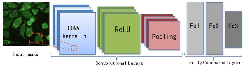
Figure 2. General scheme
2. General scheme of
of the
the architecture
architecture of
of aa the
the Convolutional
Convolutional Neural
Neural Network
Network (CNN).
(CNN).
3.4. Pre-Trained CNNs
Considering the state-of-the-art methods for CNNs, we have chosen the following four
architectures:
AlexNet [10]: the AlexNet network is one of the first convolutional neural networks that hasAppl. Sci. 2020, 10, 6940 10 of 20
The capacity of a CNN can vary based on the number of layers it has. In addition to having
different types of layers, a CNN can have multiple layers of the same type. In fact, there is rarely a
single convolutional level, unless the network in question is extremely simple. Usually a CNN has a
series of convolutional levels, the first of these, starting from the input level and going towards the
output level, is used to obtain low-level characteristics, such as horizontal or vertical lines, angles,
various contours, etc. The levels closest to the output level produce high-level characteristics, i.e.,
they represent rather complex figures such as faces, specific objects, a scene, etc. Since the design and
training of a CNN is a complex problem, where exhaustive research cannot be used, and training
requires large and accurate databases for training, and a computing power that is not always accessible
to researchers, a well-established way in the literature is to use pre-trained CNN networks. Thanks to
ImageNet competition, extremely powerful CNN networks have emerged [38]. These CNNs have
been trained on over a million images to model generic feature rich representations.
In this work, CNNs were used to classify the fluorescence intensity in HEp-2 images. In detail,
the performances of four of the most well-known pre-trained CNNs were analyzed applying them
according to the fine-tuning learning approach. The strategy according to which pre-trained networks
are used as feature extractors was also evaluated. In this case, the classification phase is usually carried
out in combination with a classifier. For this purpose, we have used linear SVM classifiers in this work.
The choice of best configuration was performed automatically, using the AUC as a figure of merit in a
validation process based on the k-fold method.
3.4. Pre-Trained CNNs
Considering the state-of-the-art methods for CNNs, we have chosen the following four architectures:
• AlexNet [10]: the AlexNet network is one of the first convolutional neural networks that has
achieved great classification successes. The winner of the 2012 Image-Net Large-Scale Visual
Recognition Challenge (ILSVRC) competition, this network was the first to obtain more than good
results on a very complex dataset such as ImageNet. This network consists of 25 layers, the part
relating to convolutional layers sees 5 levels of convolution with the use of ReLU and (only for the
first two levels of convolution and for the fifth) the max pooling technique. The second part of the
CNN is composed of fully connected layers with the use of ReLU and Dropout techniques and
finally by softmax for a 1000-d output.
• SqueezeNet [39]: in 2016 the architecture of this CNN was designed to have performances
comparable to AlexNet, but with fewer parameters, so as to have an advantage in distributed
training, in exporting new models from the cloud, and in deployment on a FPGA with limited
memory. Specifically, this network consists of 68 layers with the aim of producing large activation
maps. The filters used instead of being 3 × 3 are 1 × 1 precisely to reduce the computation by 1/9.
CNN is made up of blocks called “fire modules”, which contain a squeeze convolution layer with
1x1 filters and a expand layer with a mix of 1 × 1 and 3 × 3 convolution filters. This CNN has an
initial and a final convolution layer, while the central part of the CNN is composed of 8 fire module
blocks. No fully connected layers are used but an average pooling before the final softmax.
• ResNet18 [40]: this CNN, introduced in 2015, and inspired by the connection between neurons
in the cerebral cortex, uses a residual connection or skip connections, which jump over some
layers. With this method, it is possible to counteract the problem of degradation of performance
as the depth of the net increases, in particular the “vanishing gradient”. This CNN is made up
of 72 layers, the various convolutions are followed by batch normalization and ReLU, while the
residual connection exploits an additional layer of two inputs. The last layers consist of an average
pooling, a fully connected layer and softmax.
• GoogLeNet [41]: this architecture is based on the use of “inception modules”, each of which
includes different convolutional sub-networks subsequently chained at the end of the module.
This network is made up of 144 layers, the inception blocks are made up of four branches, the first
three with 1 × 1, 3 × 3, and 5 × 5 convolutions, and the fourth with 3 × 3 max pooling. After that,Fine-tuning is a transfer learning technique that focuses on storing knowledge gained while
solving one problem and applying it to a different but related problem [42]. Since CNNs are
composed of numerous layers and a huge number of parameters, e.g., AlexNet has 650 K neurons
and 60 M parameters (as an example, a graphical representation of the AlexNet architecture is shown
in Figure
Appl. 3),10,the
Sci. 2020, network training phase should benefit from the use of databases rich in examples
6940 11 of 20
that avoid the problem of overfitting. Unfortunately, it is not always possible to take advantage of
such large databases. Furthermore, training a CNN effectively better on a large database is
all feature
demanding both maps at different
in terms paths aretime
of computation concatenated together as the
and the computational input of
resources the next module.
required.
The last layers are composed of an average pooling and a fully
Fine-tuning arises from the need to make up for these deficiencies. This method connected layers and the softmax
consists in the
for the final output.
possibility of using a Neural Network, pre-trained on a large database, through a further training
phase with another database, even a small one. The output level is replaced with a new softmax
3.5. Fine-Tuning Description
output level, adjusting the number of classes to the classification problem being faced. The initial
Fine-tuning
values of the weights is a transfer
used arelearning
those of technique that focuses
the pre-trained network, onexcept
storing forknowledge gained
the connections while
between
solving one problem
the penultimate and and applying
last level whoseit toweights
a different but relatedinitialized.
are randomly problem [42]. New Since CNNs
training are composed
iterations (SGD)
of numerous layers and a huge number of parameters, e.g., AlexNet has 650
are performed to optimize the weights with respect to the peculiarities of the new dataset (it does K neurons and 60not
M
parameters
need to be (as an example,
large). a graphical
Fine-tuning can be representation
done in two ways. of theOne
AlexNet
way architecture
is to freeze is
theshown in Figure
weights of some3),
the network
layers and carry training phase
out new should
training benefit
cycles from the
to modify theuse of databases
weights rich in examples
of the remaining thatconcept
layers. The avoid
the problem
of fixing the of overfitting.
weights of theUnfortunately,
layers is defined it isasnot alwaysofpossible
freezing to take
the layers. advantage
Generally, theyofare
such
thelarge
first
databases.
layers to beFurthermore,
frozen as thetraining a CNN
first layers effectively
capture better
low level on a large
features. Thedatabase
greater is
thedemanding
number ofbothfrozenin
terms
layers,ofthe
computation time andeffort
less the fine-tuning the computational
in terms of time resources required.
and resources is required.
Figure 3.3. Schematic
Figure Schematic of
of the
the AlexNet
AlexNet architecture.
architecture. The
The output
output has
has been
been replaced
replaced considering
considering the
the two
two
classes on which to discriminate.
classes on which to discriminate.
Fine-tuning arises from the need to make up for these deficiencies. This method consists in the
possibility of using a Neural Network, pre-trained on a large database, through a further training
phase with another database, even a small one. The output level is replaced with a new softmax output
level, adjusting the number of classes to the classification problem being faced. The initial values of the
weights used are those of the pre-trained network, except for the connections between the penultimate
and last level whose weights are randomly initialized. New training iterations (SGD) are performed to
optimize the weights with respect to the peculiarities of the new dataset (it does not need to be large).
Fine-tuning can be done in two ways. One way is to freeze the weights of some layers and carry out
new training cycles to modify the weights of the remaining layers. The concept of fixing the weights of
the layers is defined as freezing of the layers. Generally, they are the first layers to be frozen as the
first layers capture low level features. The greater the number of frozen layers, the less the fine-tuning
effort in terms of time and resources is required.
In this case, the weights of the first CNN levels are frozen and the remaining parameters/weights are
trained. The other way is to have the architecture re-train entirely on the new database. This method
is called training from scratch. It is intuitive that the greater the number of frozen layers the
lower the computational cost of training, so training from scratch is the most expensive form of
computational training.
3.6. Hyperparameter Optimization
The design of a generic CNN provides, in addition to establishing the architecture and the
topology, the optimization of parameters and connection weights through optimization procedures in
the training phase. It refers to the numerous values to be optimized as hyperparameters optimization.Appl. Sci. 2020, 10, 6940 12 of 20
The pre-trained CNNs have a consolidated and optimized architecture for the database for which they
were originally trained.
The process of optimizing the parameters during the training phase is certainly not trivial.
Among the most recognized methods, there is the Stochastic Gradient Descent with Momentum
(SGDM) that minimizes the loss function at each iteration considering the gradient of the loss function
on the entire training dataset. The momentum term reduces the oscillations of the SGDM algorithm
along the path of steepest descent towards the optimum. The momentum is responsible for reducing
some noise and oscillations in the high curvature regions of the loss function generated by the SGD.
A variant of the SGD uses training subsets called mini-batches, in this case a different mini-batch is
used at each iteration. Simply put, the mini-batch specifies how many images to use in each iteration.
The full pass of the training algorithm over the entire training set using mini-batches is one epoch.
SGDM with mini-batch was used in this work.
Another fundamental parameter of the training process is the learning rate that allows to
set the learning speed of the training process with the level of improvement of the network’s
weights. Conceptually, a high learning rate increases the speed of training execution by sacrificing
the performance of the trained network, while a low learning rate will increase the training times by
optimizing the network’s weights that will be more performing. This parameter defines the level
of adjustments of weight connections and network topology applied at each training cycle. A small
learning rate permits a surgical fine-tune of the model to the training data, at the cost of a greater
number of training cycles and longer processing times. A high learning rate permits the model to
learn more quickly, but may sacrifice its accuracy caused by the lack of precision over the adjustments.
This parameter is generally set to 0.01, but in some cases, it is interesting to be fine-tuned, especially
when it is necessary to improve the runtime when using SGD. Table 2 shows the search space analyzed
for the optimization of the parameters.
Table 2. Hyperparameters grid search.
Parameter Configurations
Stochastic Gradient Descent with Momentum with
Training mode
mini-batch
Mini-batch size {4, 8, 16, 32, 64, 128, 256}
Learning Rate {0.01, 0.001, 0.0001}
Momentum coefficient 0.9
max 10 epoch if freeze some layers max 30 epoch if
Epoch
training CNN from scratch
The extraction of features from a pre-trained CNN is simple to implement and computationally
fast as it exploits the implicit power of representing CNN characteristics. In this work, the feature
vector extracted from the generic CNN is used to train a SVM classifier. As the size of the feature vector
is large, we have chosen to train a linear SVM that has one hyperparameter: the penalty parameter “C”
of the error term. The search for linear kernel parameter “C” is carried out using MATLAB “logspace”
function in the range [10−6 , 102.5 ]; twenty equidistant values on a logarithmic scale were analyzed.
3.7. Training Strategy and Classification
In this work the binary classification of HEp-2 images in positive and negative fluorescence intensity
was analyzed. In this regard, the transfer learning technique was used on CNN pre-trained networks.
In detail, the fine-tuning approach was analyzed for each CNN network, according to which,
starting from the generic pre-trained CNN, the parameters are optimized by carrying out a training
using the new database. In general, to implement fine-tuning, the last layer must be replaced toAppl. Sci. 2020, 10, x FOR PEER REVIEW 12 of 19
3.7. Training Strategy and Classification
Appl. Sci. 2020, 10, 6940
In this 13 of 20
work the binary classification of HEp-2 images in positive and negative fluorescence
intensity was analyzed. In this regard, the transfer learning technique was used on CNN pre-trained
networks.
correctly define thethe
In detail, number of classes
fine-tuning to be was
approach discriminated.
analyzed forTheeachproblem analyzed
CNN network, in this work,
according since we
to which,
want starting
to discriminate between two classes, turns out to be binary.
from the generic pre-trained CNN, the parameters are optimized by carrying out a training
In the the
using present
new work, the In
database. four CNN networks
general, to implementdescribed in Section
fine-tuning, 3.4layer
the last havemust
been beanalyzed,
replacedtraining
to
themcorrectly
both in scratch mode
define the andofwith
number fine-tuning
classes considering
to be discriminated. Thethree different
problem depths
analyzed ofwork,
in this freeze. Table 3
since
showswethe
want to discriminate
three freeze levelsbetween
chosentwo
for classes, turns out to be binary.
each CNN.
In the present work, the four CNN networks described in Section 3.4 have been analyzed,
training themTable Number
3. in
both scratchof frozen
mode andlayers
withat different levels
fine-tuning and forthree
considering the CNN analyzed.
different depths of freeze.
Table 3 shows the three freeze levels chosen for each CNN.
CNN Name Total Layers Low Frozen Medium Frozen High Frozen
AlexNet 25
Table 3. Number of frozen 9
layers at different levels and 16 19
for the CNN analyzed.
SqueezeNet 68 11 34 62
CNN Name Total Layers Low Frozen Medium Frozen High Frozen
ResNet18
AlexNet 2572 12
9 52 16 67 19
SqueezeNet
GoogLeNet 68144 11 11034 139 62
ResNet18 72 12 52 67
GoogLeNet 144 11 110 139
As an example, Figure 4 shows the 25 layers that make up the AlexNet CNN with the graphic
overlay ofAs the
anthree frozen
example, levels
Figure chosen
4 shows theto25perform themake
layers that fine-tuning. The first
up the AlexNet CNN level
withcalled low frozen
the graphic
indicates
overlay of the three frozen levels chosen to perform the fine-tuning. The first level called low frozenof the
that the weights of the first nine layers of CNN AlexNet are fixed with the values
network pre-trained
indicates on the original
that the weights of the firstImageNet
nine layersdatabase.
of CNN AlexNetThe fine-tuning
are fixed within this case consists
the values of the in
network
applying pre-trained
training cycles toonCNN
the original ImageNet
by changing database.ofThe
the weights the fine-tuning in this at
remaining layers case
eachconsists in i.e.,
iteration,
from applying
layer 10 training cycles
to the last. In to CNNsimilar
a very by changingway the weights
to the of the the
first level, remaining
medium layers at each
frozen anditeration,
high frozen
levelsi.e.,
werefrom layerinto
taken 10 to the last. In a very
consideration, which, similar way to thefix
respectively, first
thelevel, the medium
weights frozen and high
of the pre-trained AlexNet
frozen levels were taken into consideration, which, respectively, fix the weights of the pre-trained
network up to layer 16 and layer 19; the fine-tuning in these two cases is carried out by modifying the
AlexNet network up to layer 16 and layer 19; the fine-tuning in these two cases is carried out by
weights of the last 9 layers and 6 layers. As described in sub-Section 3.6, the three selected fine-tuning
modifying the weights of the last 9 layers and 6 layers. As described in sub-Section 3.6, the three
levelsselected
are analyzed by iterating
fine-tuning levels areonanalyzed
the learning rate values
by iterating on the{0.01, 0.001,rate
learning 0.0001}
valuesand on 0.001,
{0.01, the various
0.0001}batch
sizes and
considering a maximum of 10 epochs. The results obtained and the related
on the various batch sizes considering a maximum of 10 epochs. The results obtained and the best configurations
are reported in the
related best next section.
configurations are reported in the next section.
Figure 4. Example
Figure diagram
4. Example of theofthree
diagram levels
the three of freezing
levels of the
of freezing weights
of the weightsreferred
referredto
tothe
the AlexNet
AlexNet layers.
layers.
Table 4 shows, by way of example, part of the code to carry out the fine-tuning of CNN AlexNet.
Table
The code is 4 shows,
written byMATLAB
using way of example,
R2020apart of the
[43] andcode to carry outconsists
conceptually the fine-tuning of CNN
of seven AlexNet.
steps.
The code is written using MATLAB R2020a [43] and conceptually consists of seven steps.
Table 4. Steps for the fine-tuning of the pre-trained AlexNet network.
Table 4. Steps for the fine-tuning of the pre-trained AlexNet network.
Step 1: load AlexNet pre-trained CNN and take input
image size. %%% load pre-trained networknetwork
Step 1: load AlexNet pre-trained %%% load pre-trained
After download and install Deep LearningCNN
Toolbox Model myNet =myNet
alexnet;= alexnet;
and takesupport
for AlexNet Network input image size.set “myNet” as
package,
%%% take%%%input image
take inputsize
image size
AlexNet CNN pre-trained on the ImageNet data set.
inputSize = myNet.Layers(1). InputSize;
set “inputSize” because AlexNet requires input images of
size 227×227×3.
Step 2: load images. %%% load training / validation / test
Load the training/validation/test images with the imdsTrain = imageDatastore(dir_training),
imageDatastore function that automatically labels the ‘IncludeSubfolders’,true, ‘LabelSource’, ‘foldernames’);
images based on folder names and stores the data as an imdsValid = imageDatastore(dir_validation),
ImageDatastore object. The imageDatastore function is ‘IncludeSubfolders’,true, ‘LabelSource’, ‘foldernames’);
optimized for large image data and efficiently read batches imdsTest = imageDatastore(dir_test),
of images during training. ‘IncludeSubfolders’,true, ‘LabelSource’, ‘foldernames’);Appl. Sci. 2020, 10, 6940 14 of 20
Table 4. Cont.
%%% resize images and augmentation with rotation
imageAugmenter =
imageDataAugmenter(‘RandRotation’,(−20,20));
Step 3: resize images and apply augmentation with rotation.
augimdsTrain = augmentedImageDatastore(inputSize(1:2),
With the augmentedImageDatastore function, the
imdsTrain, ‘DataAugmentation’, imageAugmenter);
training/validation/test images are resized and augmented
augimdsValid = augmentedImageDatastore(inputSize(1:2),
with rotation of 20◦ .
imdsValid, ‘DataAugmentation’, imageAugmenter);
augimdsTest = augmentedImageDatastore(inputSize(1:2),
imdsTest, ‘DataAugmentation’, imageAugmenter);
%%% replace final layers
Step 4: replace final layers.
layersTransfer = myNet.Layers(1:end-3);
Replace final layers considering that the new classes are
layers = (layersTransfer fullyConnectedLayer (2) % two
only positive and negative while the pre-trained AlexNet
class: positive and negative softmaxLayer
are configured for 1000 classes.
classificationLayer);
Step 5: freeze initial layers.
%%% freeze initial layers
With the freezeWeights function, the first network layers
freeze = 16; % the first 16 layers layers(1:freeze) =
chosen are frozen so the new training does not change
freezeWeights(layers(1:freeze));
these weights.
%%% training options
Step 6: training network.
options = trainingOptions(‘sgdm’, . . . % sgd with
”Option” set the various training parameters such as the
momentum
optimization algorithm, the learning rate, etc. The function
‘MiniBatchSize’, 32, ‘MaxEpochs’, 10, . . . ‘LearnRate’, 0.001,
trainNetwork executes the training on the network
. . . ‘Momentum’, 0,9, . . . ‘ValidationData’, augimdsValid’);
“myNet” considering the options, the freeze weights and
%%% train network using the training and validation data
the validation images set.
myNet = trainNetwork(augimdsTrain, layers, options);
%%% test network fine tuned
Step 7: test network. [pred, probs] = classify(myNet, augimdsTest);
With the classify function, the network trained on the %%% extract performance
validation set is tested on the test set, and the performance (X,Y,T,AUC) = perfcurve(imdsTest.Labels, probs, ‘POS’);
measures are extracted, such as ACC and AUC. Perfcurve fprintf(‘ACC: %d\n’, accuracy); %print ACC
function find the AUC and then the ROC curve is drawn fprintf(‘AUC: %d\n’, AUC); %print AUC
with plot function. figure, plot(X,Y,‘r’); %ROC curve
accuracy = mean(pred == imdsTest.Labels);
4. Results
This section reports the procedures carried out and the results obtained regarding the classification
of the fluorescence intensity in the positive/negative classes of the HEp-2 images with the fine-tuning
method. For a better evaluation of the results, a comparison was made with the results obtained by the
same CNNs used by feature extractors and finally a comparison with other state-of-the-art methods.
For the four pre-trained CNN networks described in Section 3.4, the transfer learning technique
applied to HEp-2 images was analyzed. The division of the available patterns was carried out with a
5-fold cross validation and for each of the 5 iterations, training, validation, and testing were performed.
The training phase was optimized considering the AUC as a measure of merit. IIF images have been
resized to 227 × 227 (for AlexNet and SqueezeNet networks) and 224 × 224 (for GoogLeNet and
ResNet18 networks) to be provided as input to CNN; no preprocessing has been applied to the image.
CNN networks want a 3-channel image input, for this reason, we have evaluated the results using
both RGB IIF images and only the green channel and replicating it on R and B channels. The results
favored the second choice, to which all of the analyses reported in this work were conducted.
Moreover, we evaluated the application of the data augmentation using the rotation with angles of
20◦ . Data augmentation is a very effective practice especially when the data set for training is limited,
or as in our case, when some classes are not particularly represented in the set of examples. In this way
an 18 times larger sample data set was obtained.
The effect of this data augmentation was valued quantitatively in terms of performance. Table 5
shows the best results obtained, in terms of AUC, from the four CNNs analyzed:You can also read