R 1270 - Asymmetry in the conditional distribution of euro-area inflation by Alex Tagliabracci - Banca d'Italia
←
→
Page content transcription
If your browser does not render page correctly, please read the page content below
Temi di discussione
             (Working Papers)

             Asymmetry in the conditional distribution of euro-area inflation

             by Alex Tagliabracci
March 2020

                                                                       1270
                                                              Number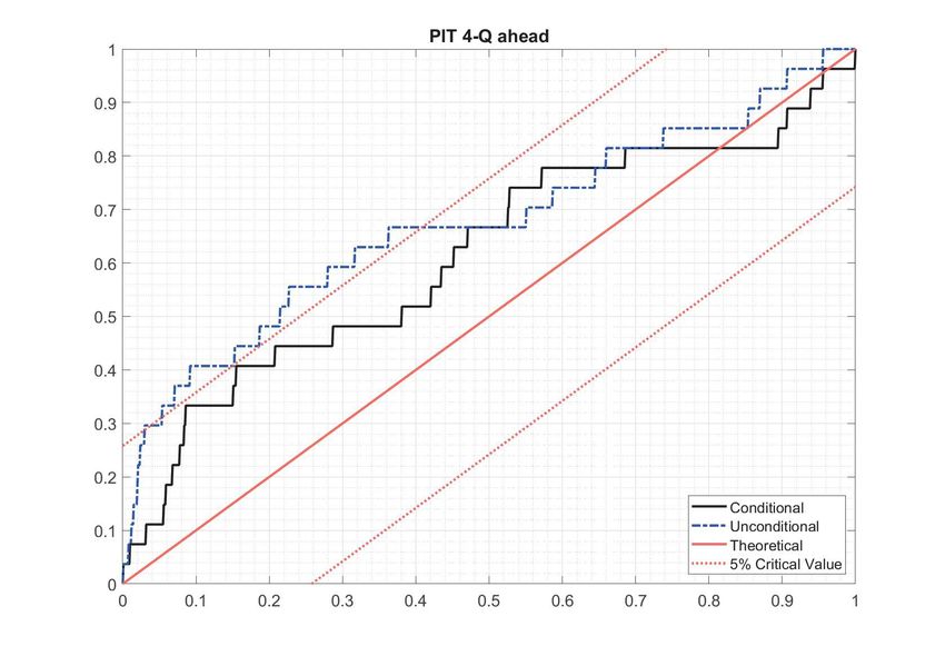
Temi di discussione
(Working Papers)

Asymmetry in the conditional distribution of euro-area inflation

by Alex Tagliabracci

Number 1270 - March 2020
The papers published in the Temi di discussione series describe preliminary results and
are made available to the public to encourage discussion and elicit comments.
The views expressed in the articles are those of the authors and do not involve the
responsibility of the Bank.

Editorial Board: Federico Cingano, Marianna Riggi, Monica Andini, Audinga
Baltrunaite, Marco Bottone, Davide Delle Monache, Sara Formai, Francesco
Franceschi, Salvatore Lo Bello, Juho Taneli Makinen, Luca Metelli, Mario
Pietrunti, Marco Savegnago.
Editorial Assistants: Alessandra Giammarco, Roberto Marano.

ISSN 1594-7939 (print)
ISSN 2281-3950 (online)
Printed by the Printing and Publishing Division of the Bank of Italy
ASYMMETRY IN THE CONDITIONAL DISTRIBUTION OF EURO-AREA INFLATION

                                                      by Alex Tagliabracci*

                                                                Abstract
Macroeconomic conditions are among the key determinants of the inflation outlook. This
paper studies how business cycles affect the conditional distribution of euro-area inflation
forecasts. Using a quantile regression approach, I estimate the conditional distribution of
inflation to assess the impact of business cycle conditions over time and the possible
asymmetries across quantiles of inflation. Interestingly, downside risks to inflation forecasts
are related to the business cycle while upside risks are instead relatively stable over time and
are not affected by the state of the economy.

JEL Classification: C32, E31, E32, E37.
Keywords: inflation, quantile regression, conditional distribution, asymmetry, downside
risks.
DOI: 10.32057/0.TD.2020.1270

                                                               Contents

1. Introduction ......................................................................................................................... 5
2. Estimating the conditional distribution................................................................................ 7
   2.1 Quantile regression approach ....................................................................................... 8
   2.2 The conditional distribution ........................................................................................ 10
   2.3 In-sample fit ................................................................................................................ 11
3. Asymmetry in inflation distribution .................................................................................. 12
   3.1 Relative entropy.......................................................................................................... 12
   3.2 Expected shortfall and longrise .................................................................................. 13
   3.3 Policy-scenario probabilities ...................................................................................... 14
4. Out-of-sample .................................................................................................................... 15
   4.1 Quantile score ............................................................................................................. 15
   4.2 Probability integral transformation ............................................................................. 16
5. Robustness checks ............................................................................................................. 18
6. Conclusions ....................................................................................................................... 19
References .............................................................................................................................. 20
Data appendix: ....................................................................................................................... 22

_______________________________________
*
    Bank of Italy, DG Economics, Statistics and Research.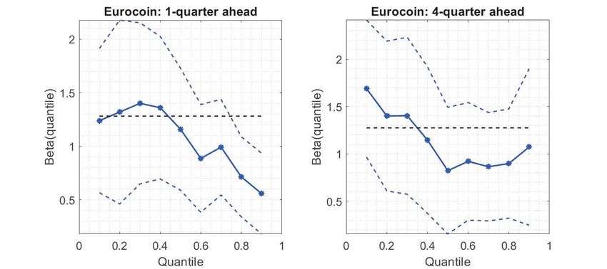

“If we look at the uncertainty dimension of inflation, we see two phe-
        nomena. The first is that tail risks have disappeared. [. . . ] And we also
        see that the uncertainty about the path of inflation has also decreased.”

                                                            Mario Draghi, 8 June 2017

1       Introduction1
Predicting inflation is of primary importance for several reasons, especially for the
conduct of monetary policy. The literature on forecasting inflation has showed an
increasing effort over the last years in better characterizing the level of uncertainty
associated to point estimates, which is generally captured by means of the predic-
tive density (e.g. Elliott and Timmermann [2008]). An accurate representation of
the possible risks related to future inflation is undoubtedly relevant both for eco-
nomic agents and policymakers. The importance of this point is clear in most of
the economic surveys: indeed, professional forecasters, and more in general market
operators participating in these questionnaires, are asked to provide not only their
point estimates but also the probability distribution of their forecasts. Similarly,
policymakers regularly evaluate the probability of different scenarios, such as de-
flation or high-inflation rate, to gauge possible risks associated to future inflation,
which is a major threat to policy effectiveness.
    Macroeconomic conditions are generally considered the major driver of inflation.
Scholars have extensively investigated how the state of the economy propagates into
the dynamics of future prices. This paper takes a step into this direction: indeed, it
contributes to the literature on inflation forecasting by providing a comprehensive
study on how macroeconomic conditions shape the conditional distribution of infla-
tion forecasts in the euro area. To do so, first it uses a quantile-regression approach
to characterize the effects of changes in the current state of the economy with re-
spect to the entire distribution of inflation. Then, it adopts the quantile function
to estimate the conditional distribution of inflation forecasts. This method follows
Adrian, Boyarchenko, and Giannone [2019] who focus on the relation between US
gross domestic product and financial conditions. Their approach fits with the pur-
pose of this paper because it allows to investigate the properties of the conditional
    1
     This paper previously circulated with the title “The Vulnerability of Euro Area Inflation Fore-
casts”. I would like to thank Andrea Gazzani, Domenico Giannone, Alberto Musso, Stefano Neri,
Andrea Nobili, Gabriel Pérez-Quirós and Roberta Zizza for their helpful comments. I also ben-
efited from comments made by participants at seminars at Universitat Autonoma de Barcelona,
ECB, IAEE 2019. All the possible errors remain mine.

                                                 5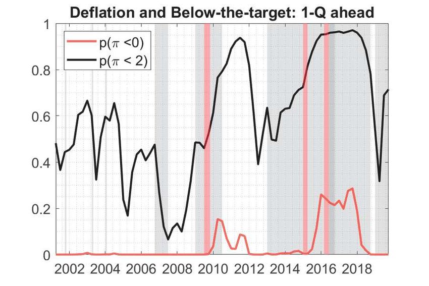
distribution, focusing not only on the first two moments, as generally done in the
literature, but rather on the entire shape of the distribution.
    Existing studies have already investigated the distribution of inflation forecasts
using a different perspective. Some examples are Tsong and Lee [2011] who show
asymmetric inflation dynamics for twelve OECD countries and Manzan and Zerom
[2013] who challenged the view that random-walk models are more accurate for
forecasting inflation by exploring the power of leading indicators of economic activity
as valuable predictors, especially at the tails of the distribution. Busetti et al. [2015]
adopt a quantile phillips-curve approach for the euro area with the aim of improving
the accuracy of standard linear forecasting models.
    This paper takes a different direction with respect to the existing literature be-
cause it does not propose a standard “horse-race” forecasting exercise for competing
models but rather it uses a quantile regression approach to estimate the conditional
distribution of inflation forecasts in the euro area and analyze its evolution over time
with respect to economic conditions. Loosely speaking, this allows to study how the
current state of the economy shapes the (model-based) uncertainty and risks asso-
ciated to future inflation. The idea is that macroeconomic conditions matter for
future inflation but in an asymmetric way, i.e. more for lower quantiles of inflation
whereas are not informative for the upper quantiles.
    The main finding of this paper is that the distribution of euro area inflation
forecasts conditional on the current state of the economy evolves asymmetrically.
Specifically, the left part of the distribution is sensitive to the deterioration of eco-
nomic conditions while the right part remains relatively stable over time, regardless
if the economy is experiencing an expansion phase. In other words, downside risks
to inflation vary considerably with the business cycle whereas upside risks are less
sensitive to economic fluctuations. This finding appears robust to a large and het-
erogeneous set of business cycle indicators commonly used to study the relation
of between prices and output. This asymmetric relation appears important also
for forecasting purpose: the performance of the model in an out-of-sample setting
is higher for lower quantiles and the accuracy gain decreases nearly monotonically
across quantiles.
    Interestingly, other previous works investigated possible determinants of inflation
risks: for instance Andrade et al. [2014] look at how financial market data affect
survey-based inflation risk indicators in the euro area and Lopez-Salido and Loria
[2019] document that financial conditions can carry substantial and persistent low-
inflation risks both in the US and in the euro area. This paper differs from them
because it focuses explicitly on the role of business cycle indicators rather than

                                            6
financial variables on the inflation outlook.
The rest of the paper is structured as follows. Section 2 illustrates the steps
to estimate the conditional distribution of inflation forecasts which is then used in
section 3 for further analyses. Section 4 performs perform an out-of-sample exercise
while and 5 presents some robustness checks. Section 6 briefly concludes.
2 Estimating the conditional distribution
Characterizing the relation between inflation and the business cycle belongs to the
long-lasting debate on the validity of the Phillips curve. To study this relation, I first
consider the data for the euro area by looking at the year-on-year inflation rate and a
business cycle variable. Specifically, I use the e-coin (Eurocoin) indicator, which is
a measure introduced by Altissimo et al. [2010] and can be considered as a real-time
“thermometer” of the euro area economy2 . The choice of using the e-coin rather
than other business cycle indicators as real GDP or unemployment rate is motivated
by the fact that the e-coin is obtained as a smooth estimate that summarizes the
current economic condition for the euro area in one index3 . Together with the year-
on-year inflation rate, data are taken at a quarterly frequency and spanned over the
period 1999Q1-2019Q3 as illustrated in figure 11.
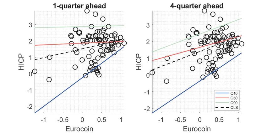
Figure 1 shows the scatter plots of the data together with the slope of 10th, 50th
and 90th percentiles and the ordinary least squares (OLS) estimates (black-dashed
line) for two different horizons, i.e. one and four quarters ahead. These charts are
informative about the ability/inability of the OLS in fitting the data at all quantiles:
for instance, if the OLS line is parallel to the ones characterizing the other quantiles,
then it indicates that a linear regression model also does a good job in capturing
the relation between inflation and e-coin in the tails.
The evidence suggests that the OLS performs poorly at both tails, especially at lower
quantiles. In particular, the 10th percentile slope (blue line) behaves remarkably
different from the other lines and this holds at both horizons. This represents a
motivating point for the adoption of the quantile regression for the remaining of this
paper.
2
In practice, this index is constructed from a dynamic factor model which uses a large set of
macroeconomic variables (industrial production, business surveys, financial and demand indicators
and others) to extract the information that is relevant to forecast GDP.
3
The results of this paper are robust to the choice of using other business cycle indicators as
shown by some evidence are presented in Section 5.
7Figure 1: Scatter plot
2.1 Quantile regression approach
The quantile regression and the simple linear regression model (OLS) mainly differs
in two ways: the minimization problem is based on the sum of absolute errors and
not on the sum of squared errors and in addition the error terms are weighted differ-
ently according to the relative quantile (and not equally as in the OLS framework).
Concretely, as shown by Adrian et al. [2019], the use of the quantile regression ap-
proach presents two main advantages. First, it allows to study the impact of the
explanatory variables on different quantiles of the inflation distribution and not only
on the mean as in the case of OLS. This feature is extremely important since recent
periods have been characterized by two recessions and simple linear regression mod-
els might fail to capture the effects of large shocks on inflation. Second, estimation
and inference in a quantile-regression framework are distribution-free and therefore
no strong assumptions are needed on the distribution of the inflation rate.
Given this background, I estimate a quantile regression (see Koenker and Bassett
[1978]) of yt (euro area headline inflation) on xt (the e-coin plus a constant). This
allows the estimation of the conditional distribution in a second step as described in
the next session. Equation 1 shows a standard quantile regression formula in which
the coefficients βτ,h are chosen to minimize the quantile weighted absolute errors as
follows
X
T
βτ,h = argmin (τ ·✶(yt ≥ xt−h βh )|yt −xt−h βτ,h |+(1−τ )·✶(yt < xt−h βh )|yt −xt−h βτ,h |)
βh ∈Rk t=1
(1)
where τ represents the different quantiles, h the forecast horizon and ✶(·) denotes
8the indicator function. In what follows, the baseline model, i.e. the one that is used
to construct the conditional distribution, uses as regressors the average inflation rate
over the last four quarters and e-coin indicator. The first term aims at capturing
the persistence of inflation (see Atkeson and Ohanian [2001]) while the second term
describes the relation with the business cycle. Similarly, Lopez-Salido and Loria
[2019] use the average inflation rate rather than the lag of inflation in conjunction
with some financial indicators to study inflation dynamics in the euro area and in
the US. The estimated coefficients of equation 1 for the conditional model are then
analyzed to characterize their variation across quantiles. The forecast horizon is
arbitrarily selected equal to one and four to provide a short and a medium-term
view of this relation. Figures 2 illustrates the coefficient estimates across all quan-
tiles, considering a grid from 0.1 to 0.9 with a 0.05-interval. First, the blue lines
show that the coefficients are generally statistically significant (with the exception
of the right tail at one-quarter ahead)4 . Second, both graphs point out significant
differences across quantiles, especially comparing the lower quantiles with the upper
quantiles. Clearly, this reinforces the idea that OLS estimates (black dashed line)
do not properly capture tails relations and therefore are less informative about tail
behaviours which are better described in a quantile-regression approach.
Figure 2: Estimated coefficients over quantiles
4
The confidence bands are obtained by estimating the variance-covariance matrix as described
in Greene [2008].
92.2 The conditional distribution
Using the estimated coefficients βτ,h from equation 1, the predicted distribution of
inflation Q̂yt+h |xt can be directly computed as
Q̂yt+h |xt (τ ) = xt βτ,h (2)
where the forecast horizon is h = 1, 4. As described before, the conditional distribu-
tion model is obtained by including in xt the average of the last four lags of inflation
and the e-coin. Note that equation 2 produces a prediction for each quantile τ at
each t which are then used to obtain the predicted distribution by means of a non-
parametric approach as the normal kernel function (e.g. D’Agostino, Giannone, and
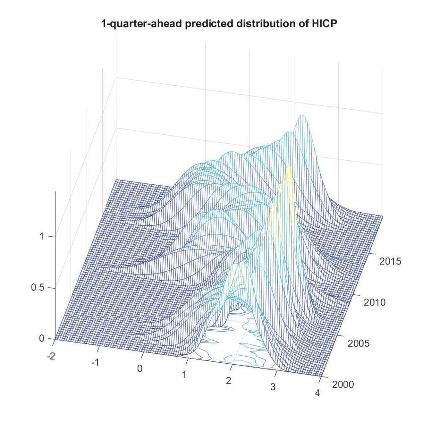
Gambetti [2013])5 . Figure 3 presents the estimated conditional distributions with
respect to one- (left) and four-quarter (right) ahead forecasts.
Figure 3: Estimated distribution of inflation forecasts
The main finding is that there is a considerable time-variation in the shape of
the conditional distribution which is mainly driven by the different behaviour of the
tails. Indeed, for both horizons, the distribution shows asymmetric moves with the
left tail more sensitive to business cycle developments while the right tail remains
relatively stable over time. Loosely speaking, the conditional distribution of infla-
tion forecasts points out that the left tail moves following business cycle conditions
5
The empirical results are robust to different approaches for estimating the conditional distri-
bution. In practice, several specifications for the kernel function or a simple linear interpolation as
in Busetti et al. [2015] produce differences across methods that are negligible.
10while the right one is more stable over time, not increasing even when the economy
goes through an expansion phase. As a consequence, this also implies that changes
in inflation uncertainty are entirely driven by the left tail of the conditional distri-
bution, therefore when an increase in the uncertainty is not generated by symmetric
moves of both tails.
2.3 In-sample fit
One way to look at the importance of business cycle indicators to explain the left
part of the distribution is to consider their contribution in terms of goodness of fit
for the tails of the distribution. To validate the (quantile regression) model, one
can use the pseudo-R2 measure suggested by Koenker and Machado [1999] which
assesses the fit at each quantile by comparing the sum of weighted deviations for
the model of interest with the same sum from a model in which only the intercept
appears, i.e.:
P P
yi ≥ŷi τ · |yi − ŷi | + (1 − τ ) · |yi − ŷi |
R (τ ) = 1 − P
2
Pyifinding characterizes the left asymmetry of this distribution and thus validates the
idea that business cycle conditions have an asymmetric effect on the conditional
distribution of inflation forecasts.
3 Asymmetry in the inflation distribution
This section examines in depth the estimated conditional distribution of inflation
to show his asymmetry in three different ways. First, it looks at the role of con-
ditioning the inflation distribution on economic conditions. Second, it provides a
quantification of the evolution of extreme inflation rate scenarios generated by the
estimated distribution. Finally, it illustrates two appealing inflation-related policy
scenarios.
3.1 Relative entropy
In this part I quantify the implications of conditioning on the state of the business
cycle by considering the Kullback-Leibler divergence between the conditional, f (y),
and the unconditional distribution, g(y), of inflation forecasts6 . As described by
Adrian et al. [2019], this measure can be used to assess the impact of the conditioning
variable on the distribution of inflation. In other words, the relative entropy provides
the information gain produced by including the current state of the business cycle.
Analytically, this can be written as
Z F −1 (0.5)
LD
t (ft , g) = (log g(y) − log ft (y)) ft (y)dy (4)
−∞
Z ∞
LUt (ft , g) = (log g(y) − log ft (y)) ft (y)dy . (5)
F −1 (0.5)
where the downside entropy LD t refers to the difference between the unconditional
and conditional distribution for the left part of the distribution (namely from the
first percentile to the median) and the upside entropy LUt which is the analogous
for the right part of the distribution. Figure 5 points out one main evidence: the
downside entropy (red line) is significantly more volatile than the upside entropy
(black line) which indeed remains stable over time. This confirms that economic
conditions do not provide any information gain about the upper quantiles of the
6
The Kullback-Leibler divergence, also known as relative entropy or information divergence, is
a measure of the non-symmetric difference between two distributions. It is generally used because
differently from other measures of distance, it has a direct counterpart in the logarithmic scoring
rule, which is commonly used for evaluating density forecasts (see Amisano and Giacomini [2007]).
12inflation distribution, while they are extremely important for the bottom ones. In
other words, the variation of the conditional distribution is mainly driven by the
movements in the left tail and not by those in the right tail which remains relatively
constant over time.
Figure 5: Downside (red) and upside (black) entropy
Note: the grey shaded areas corresponds to the CEPR recession periods in the euro area
3.2 Expected shortfall and longrise
The estimated conditional distribution can also be used to quantify the expected
values of extreme scenarios, namely either low or high values of inflation that a
forecaster might predict according to this quantile-regression model. This is imple-
mented by considering the expected shortfall and expected longrise which are two
measures commonly used in the finance literature to represent the expected return
on the portfolio in the worst (or best) τ % of cases. In practice, these two measures
can be defined as
Z 0.05 Z 1
−1
SFt = Ft (τ ) dτ LRt = Ft−1 (τ ) dτ (6)
0 0.95
and they correspond to the integral of the inverse cumulative distribution function
Ft−1 (·) at its extreme 5-percentile tails, i.e. from 1 to the 5-th percentile and from
95-th to the 100 percentile.
Figure 6 shows that for both horizons the expected longrise remains roughly stable
over time fluctuating around values of 3% while the expected shortfall is much more
volatile in the interval between -1% and 1%. The main message of these two figures
is that the expectation of low inflation is sensitive to the fluctuations in the business
cycle whereas the upside risk is less responsive to changes in economic conditions.
13Figure 6: Expected Shortfall (red) and Longrise (black)
Note: the grey shaded areas corresponds to the CEPR recession periods in the euro area
3.3 Policy-scenario probabilities
Price stability is the main target of the majority of central banks. In the euro area,
the European Central Bank (ECB) is the institution which pursues medium- and
long-term price stability, with the mandate to keep headline inflation “close but
below to two percent”. Recent episodes as the Europe’s Double-Dip recessions and
oil turmoils in the period 2014-2015 had a considerable impact on the level of prices
and brought the inflation rate also in negative territory.
With this is mind, this section uses the estimated conditional distribution to propose
the quantification of two relevant policy scenarios, namely the risk of deflation (π <
0) and the probability of being below the target (π < 2), which for simplicity is
assumed to be at a 2 percent inflation rate. Using the same notation of equation 6,
this can be specified as
Z (0) Z (2)
FtDEF L (0) = ft (y)dy FtBT (2) = ft (y)dy . (7)
−∞ −∞
where ft (y) is the conditional distribution of inflation and FtDEF L,BT (·) is the cor-
responding cumulative distribution function. Figure 6 illustrates the quantitative
results in following way: the red line represents the probability of a future inflation
rate in negative territory while the black line corresponds to the probability of an
inflation rate below the 2% target. Similarly, the red and the grey shaded areas
represent the periods in which the euro area was in deflationary time and below the
target, respectively.
The charts present similar results for both horizons. The probability of being
below the target is well-captured: indeed, the odds of having inflation below 2%
is generally above 0.5 for all the period after 2013, which is commonly known as
14Figure 7: Policy-scenario analysis
Note: the red shaded areas correspond to deflationary periods and the grey shaded areas represent
the periods in which the inflation rate was below 2%.
“missing inflation”. Similarly, the probability of deflation rises in 2009 related to
the severity of the recession and then it spikes again in 2016 in the period of very
low inflation due to some turmoil in oil dynamics.
4 Out-of-sample
The empirical results presented so far are obtained using an in-sample estimation
approach. Although this is extremely useful for understanding the properties of
the estimated distribution of inflation forecasts, it does not fully replicate the true
experience of a forecaster. For this reason, this section proposes an out-of-sample
exercise to assess the forecasting abilities of this quantile model. The forecasting
exercise evaluates the performance of the model over a period of seven years, i.e. 28
quarters between 2012Q4 and 2019Q3, using a recursive estimation procedure with
a focus on two specific dimensions: (i) the quantile score, which assesses the forecast
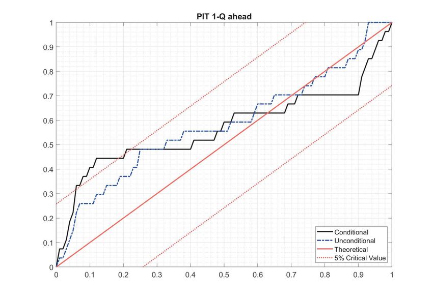
accuracy across different quantiles, and (ii) the probability integral transformation
(PIT), that measures the calibration of the predictive density.
4.1 Quantile score
In the case of a non-parametric distribution, the standard approach to evaluate
the performance of a model is to use the predictive score which corresponds to
the value of the predictive density generated by the model at the realized value of
inflation following the logic that the higher the score, the more accurate the model is.
However, in the presence of a considerable asymmetry as in this case, looking at the
score per sè is not very informative. Indeed, the most appropriate way to evaluate
these model is to assess the specific performance across quantiles (see Gneiting and
15Raftery [2007] and Busetti et al. [2015]). In practice, this corresponds to consider
the loss function L(τ ) evaluated as
X X
L(τ ) = τ |yt − Q̂τ,t | + (1 − τ )|yt − Q̂τ,t | (8)
yt ≥Qτ,t ytwhether the generated distribution zt+h , which is obtained as
Z yt+h
zt+h = ft+h (yt+h )dy, (9)
−∞
is distributed as an iid Uniform (0, 1) distribution. To test for the correct specifi-
cation of the conditional predictive density, I adopt the test proposed by Rossi and
Sekhposyan [2019] which preserves the estimation error of the parameters used to
construct the densities and focuses on evaluating the absolute performance of the
model’s predictive density7 . In this context, a perfectly calibrated density should be
equal to the 45-degree line, therefore any deviation from the bisector line suggests a
bias in the predictive density. Figure 9 shows the results for the conditional (black
line) and unconditional (blue dashed line) distribution together with the critical val-
ues (red dotted lines). A line outside these 5% critical values indicates the rejection
of the null hypothesis of correct calibration, therefore considering the model as not
correctly calibrated.
Figure 9: Probability integral transformation
Interestingly, the overall difference in terms of calibration between the two dis-
tributions is relatively small. However, for the horizon h = 1 the test rejects the null
hypothesis of correct calibration for the conditional distribution due to the left part
of the distribution. Viceversa, the null hypothesis is rejected only for the uncondi-
tional distribution for h = 4. One explanation of these results is that the business
cycle conditions lead the conditional model to be relatively pessimist on the infla-
tion outlook, generating a left asymmetry. In the second case, the lack of correct
calibration is probably due to the persistency of inflation.
7
Critical values (red dotted lines in the graphs) are obtained using the method proposed by
Rossi and Sekhposyan [2019] which also provide an interesting review of the related literature.
175 Robustness checks
The results obtained so far are based on the e-coin as the indicator of the busi-
ness cycle in the euro area. Although its validity has been extensively analyzed
(see Altissimo et al. [2010]), it is interesting to study whether the left asymmetry
of the distribution of inflation forecasts is also robust to other main business cycle
variables. For this reason, the analysis of Section 3 is repeated by conditioning on a
list of standard business cycle indicators for the euro area: more precisely, I consider
real GDP, industrial production, unemployment rate and ISM PMI manufacturing
index8 . To assess the robustness of the results, figure 10 presents the pseudo R-
squared statistic as in section 2.3. In this case, the pseudo-R2 of the unconditional
and the conditional model are compared to the corresponding values for the models
with the other business cycle indicators. These two charts confirm the main result of
the paper, namely the existence of an left asymmetry in the distribution of inflation
forecasts which is generated by the deterioration of the business cycle. In some cases
the evidence of a left asymmetry appears less strong than the case of the e-coin
but this is due to the fact that the latter is obtained by including a large variety of
indicators of business cycle, therefore it appears to better capture the current state
of the economy.
Figure 10: Robustness over business cycle indicators
8
A complete description of the variables is available in the Data Appendix.
186 Conclusions
Recent years of low inflation rates have posed new important questions for scholars
(see Ciccarelli and Osbat [2017] for the euro area). Evaluating possible risks to
inflation has become of primary importance, especially for policymakers. Quanti-
tatively, this is commonly measured by the predictive density which corresponds to
an estimate of the expected probability distribution of the target variable.
This paper proposes a comprehensive analysis of the evolution of the distribution
of inflation forecasts conditional on macroeconomic conditions to formally evaluate
the risk to inflation conditional on the current state of the economy. More specifi-
cally, I first adopt a quantile-regression approach to appropriately capture the effects
of changes in economic conditions on all quantiles of the inflation distribution. Then,
I use the quantile function to estimate the conditional distribution of inflation fore-
casts. The main finding is that there is a significant time-variation in the shape of
the distribution which is mainly due to the relation of the lower quantiles of infla-
tion with the business cycle. In other words, the conditional distribution presents a
dynamics of the downside risk which is sensitive to the current state of the economy
while the upside risk remains stable over time. This evidence is generally robust to
several business cycle indicators.
This paper also performs some other interesting exercises using the estimated
conditional distribution. First, it shows the implication of conditioning on the busi-
ness cycle by means of the relative entropy. Second, it quantifies the probability of
possible but extreme inflation outcomes and lastly it performs some relevant policy
scenario analyses to study the ability of the model in capturing inflation dynamics.
Last but not least, the main finding of this paper might have some important
policy implications. The asymmetric behaviour of the inflation distribution might
be related to the different effectiveness of the monetary policy. Indeed, the evidence
of this paper supports the idea that the central bank seems more in control of prices
during period of booms, while it appears somehow less effective during downturns,
since it can not avoid the possibility of periods of low inflation. However, the
sensitivity of this point and the centrality for policy purposes represent a stimulating
point for future research.
19References
Adrian, T., N. Boyarchenko, and D. Giannone (2019): “Vulnerable
Growth,” American Economic Review, 109, 1263–1289.
Altissimo, F., R. Cristadoro, M. Forni, M. Lippi, and G. Veronese
(2010): “New Eurocoin: Tracking Economic Growth in Real Time,” The Review
of Economics and Statistics, 92, 1024–1034.
Amisano, G. and R. Giacomini (2007): “Comparing density forecasts via
Weighted Likelihood Ratio Tests,” Journal of Business and Economic Statistics,
25, 177–190.
Andrade, P., V. Fourel, E. Ghysels, and J. Idier (2014): “The financial
content of inflation risks in the euro area,” International Journal of Forecasting,
30, 648–659.
Atkeson, A. and L. E. Ohanian (2001): “Are Phillips curves useful for fore-
casting inflation?” Quarterly Review, 2–11.
Busetti, F., M. Caivano, and L. Rodano (2015): “On the conditional distri-
bution of euro area inflation forecast,” Temi di discussione (Economic working
papers) 1027, Bank of Italy.
Ciccarelli, M. and C. Osbat (2017): “Low inflation in the euro area: Causes
and consequences,” ECB Working Papers 181, European Central Bank.
D’Agostino, A., D. Giannone, and L. Gambetti (2013): “Macroeconomic
Forecasting and Structural Change,” Journal of Applied Econometrics, 28, 82–
101.
Diebold, F. X., T. A. Gunther, and A. S. Tay (1998): “Evaluating Den-
sity Forecasts with Applications to Financial Risk Management,” International
Economic Review, 39, 863–883.
Elliott, G. and A. Timmermann (2008): “Economic Forecasting,” Journal of
Economic Literature, 46, 3–56.
Gneiting, T. and A. E. Raftery (2007): “Strictly Proper Scoring Rules, Pre-
diction, and Estimation,” Journal of the American Statistical Association, 102,
359–378.
20Greene, W. H. (2008): Econometric Analysis, International Student Edition,
Fifth Edition.
Koenker, R. and G. Bassett (1978): “Regression Quantiles,” Econometrica,
33–50.
Koenker, R. and J. Machado (1999): “Goodness of Fit and Related Inference
Processes for Quantile Regression,” Journal of the American Statistical Associa-
tion, 94, 1296–1310.
Lopez-Salido, J. and F. Loria (2019): “Inflation at Risk,” Working Paper
Series 14074, Centre for Economic Policy Research.
Manzan, S. and D. Zerom (2013): “Are macroeconomic variables useful for fore-
casting the distribution of U.S. inflation?” International Journal of Forecasting,
29, 469–478.
Rossi, B. and T. Sekhposyan (2019): “Alternative tests for correct specification
of conditional predictive densities,” Journal of Econometrics, 208, 638–657.
Tsong, C.-C. and C.-F. Lee (2011): “Asymmetric inflation dynamics: Evidence
from quantile regression analysis,” Journal of Macroeconomics, 33, 668–680.
21Data Appendix
The data are taken from the ECB Statistical Data Warehouse. The sample covers
the period Q1.1999-Q3.2019, using quarterly observations.
• HICP: Euro area (changing composition) - HICP - Overall index, Monthly in-
dex, backdated, fixed euro conversion rate used for weights, European Central
Bank, Working day and seasonally adjusted;
• e-coin: Euro area (changing composition), Centre for Economic Policy Re-
search and Banca d‘Italia, Coincident indicator of business cycle, based on
quarterly changes in cyclical component of the GDP, see Altissimo et al. [2010];
For the robustness exercise:
• real GDP Gross domestic product at market prices - Euro area 19 (fixed
composition) Chain linked volume (rebased), Non transformed data, Calendar
and seasonally adjusted data;
• ISM PMI Manufacturing: Euro area 19 (fixed composition), Markit, Man-
ufacturing - output, Total, Seasonally adjusted, not working day adjusted;
• Industrial production: Euro area 19 (fixed composition) - Industrial Pro-
duction Index, Total Industry (excluding construction); Working day and sea-
sonally adjusted;
• Unemployment rate: Euro area 19 (fixed composition) - Standardised un-
employment, Rate, Seasonally adjusted, not working day adjusted, percentage
of civilian workforce;
• Oil price index: annual growth rate of the Brent oil price converted in Euro;
• ECB commodity price index: annual growth rate of the ECB commod-
ity price index, import weighted, Euro denominated, neither seasonally nor
working day adjusted.
22Figure 11: Raw data
Data for the section on robustness checks
Note: the grey shaded areas corresponds to the recession periods in the euro area as defined by
the CEPR business cycle dating committee.
23RECENTLY PUBLISHED “TEMI” (*)
N. 1246 – Financial development and growth in European regions, by Paola Rossi and Diego
Scalise (November 2019).
N. 1247 – IMF programs and stigma in Emerging Market Economies, by Claudia Maurini
(November 2019).
N. 1248 – Loss aversion in housing assessment among Italian homeowners, by Andrea
Lamorgese and Dario Pellegrino (November 2019).
N. 1249 – Long-term unemployment and subsidies for permanent employment, by Emanuele
Ciani, Adele Grompone and Elisabetta Olivieri (November 2019).
N. 1250 – Debt maturity and firm performance: evidence from a quasi-natural experiment,
by Antonio Accetturo, Giulia Canzian, Michele Cascarano and Maria Lucia Stefani
(November 2019).
N. 1251 – Non-standard monetary policy measures in the new normal, by Anna Bartocci,
Alessandro Notarpietro and Massimiliano Pisani (November 2019).
N. 1252 – The cost of steering in financial markets: evidence from the mortgage market, by
Leonardo Gambacorta, Luigi Guiso, Paolo Emilio Mistrulli, Andrea Pozzi and
Anton Tsoy (December 2019).
N. 1253 – Place-based policy and local TFP, by Giuseppe Albanese, Guido de Blasio and
Andrea Locatelli (December 2019).
N. 1254 – The effects of bank branch closures on credit relationships, by Iconio Garrì
(December 2019).
N. 1255 – The loan cost advantage of public firms and financial market conditions: evidence
from the European syndicated loan market, by Raffaele Gallo (December 2019).
N. 1256 – Corporate default forecasting with machine learning, by Mirko Moscatelli, Simone
Narizzano, Fabio Parlapiano and Gianluca Viggiano (December 2019).
N. 1257 – Labour productivity and the wageless recovery, by Antonio M. Conti, Elisa
Guglielminetti and Marianna Riggi (December 2019).
N. 1258 – Corporate leverage and monetary policy effectiveness in the Euro area, by Simone
Auer, Marco Bernardini and Martina Cecioni (December 2019).
N. 1259 – Energy costs and competitiveness in Europe, by Ivan Faiella and Alessandro
Mistretta (February 2020).
N. 1260 – Demand for safety, risky loans: a model of securitization, by Anatoli Segura
and Alonso Villacorta (February 2020).
N. 1261 – The real effects of land use regulation: quasi-experimental evidence from a
discontinuous policy variation, by Marco Fregoni, Marco Leonardi and Sauro
Mocetti (February 2020).
N. 1262 – Capital inflows to emerging countries and their sensitivity to the global
financial cycle, by Ines Buono, Flavia Corneli and Enrica Di Stefano (February 2020).
N. 1263 – Rising protectionism and global value chains: quantifying the general equilibrium
effects, by Rita Cappariello, Sebastián Franco-Bedoya, Vanessa Gunnella
and Gianmarco Ottaviano (February 2020).
N. 1264 – The impact of TLTRO2 on the Italian credit market: some econometric evidence,
by Lucia Esposito, Davide Fantino and Yeji Sung (February 2020).
N. 1265 – Public credit guarantee and financial additionalities across SME risk classes,
by Emanuele Ciani, Marco Gallo and Zeno Rotondi (February 2020).
(*) Requests for copies should be sent to:
Banca d’Italia – Servizio Studi di struttura economica e finanziaria – Divisione Biblioteca e Archivio storico – Via
Nazionale, 91 – 00184 Rome – (fax 0039 06 47922059). They are available on the Internet www.bancaditalia.it."TEMI" LATER PUBLISHED ELSEWHERE
2018
ACCETTURO A., V. DI GIACINTO, G. MICUCCI and M. PAGNINI, Geography, productivity and trade: does
selection explain why some locations are more productive than others?, Journal of Regional Science,
v. 58, 5, pp. 949-979, WP 910 (April 2013).
ADAMOPOULOU A. and E. KAYA, Young adults living with their parents and the influence of peers, Oxford
Bulletin of Economics and Statistics,v. 80, pp. 689-713, WP 1038 (November 2015).
ANDINI M., E. CIANI, G. DE BLASIO, A. D’IGNAZIO and V. SILVESTRINI, Targeting with machine learning:
an application to a tax rebate program in Italy, Journal of Economic Behavior & Organization, v.
156, pp. 86-102, WP 1158 (December 2017).
BARONE G., G. DE BLASIO and S. MOCETTI, The real effects of credit crunch in the great recession: evidence from
Italian provinces, Regional Science and Urban Economics, v. 70, pp. 352-59, WP 1057 (March 2016).
BELOTTI F. and G. ILARDI Consistent inference in fixed-effects stochastic frontier models, Journal of
Econometrics, v. 202, 2, pp. 161-177, WP 1147 (October 2017).
BERTON F., S. MOCETTI, A. PRESBITERO and M. RICHIARDI, Banks, firms, and jobs, Review of Financial
Studies, v.31, 6, pp. 2113-2156, WP 1097 (February 2017).
BOFONDI M., L. CARPINELLI and E. SETTE, Credit supply during a sovereign debt crisis, Journal of the
European Economic Association, v.16, 3, pp. 696-729, WP 909 (April 2013).
BOKAN N., A. GERALI, S. GOMES, P. JACQUINOT and M. PISANI, EAGLE-FLI: a macroeconomic model of
banking and financial interdependence in the euro area, Economic Modelling, v. 69, C, pp. 249-
280, WP 1064 (April 2016).
BRILLI Y. and M. TONELLO, Does increasing compulsory education reduce or displace adolescent crime?
New evidence from administrative and victimization data, CESifo Economic Studies, v. 64, 1, pp.
15–4, WP 1008 (April 2015).
BUONO I. and S. FORMAI The heterogeneous response of domestic sales and exports to bank credit shocks,
Journal of International Economics, v. 113, pp. 55-73, WP 1066 (March 2018).
BURLON L., A. GERALI, A. NOTARPIETRO and M. PISANI, Non-standard monetary policy, asset prices and
macroprudential policy in a monetary union, Journal of International Money and Finance, v. 88, pp.
25-53, WP 1089 (October 2016).
CARTA F. and M. DE PHLIPPIS, You've Come a long way, baby. Husbands' commuting time and family labour
supply, Regional Science and Urban Economics, v. 69, pp. 25-37, WP 1003 (March 2015).
CARTA F. and L. RIZZICA, Early kindergarten, maternal labor supply and children's outcomes: evidence
from Italy, Journal of Public Economics, v. 158, pp. 79-102, WP 1030 (October 2015).
CASIRAGHI M., E. GAIOTTI, L. RODANO and A. SECCHI, A “Reverse Robin Hood”? The distributional
implications of non-standard monetary policy for Italian households, Journal of International Money
and Finance, v. 85, pp. 215-235, WP 1077 (July 2016).
CIANI E. and C. DEIANA, No Free lunch, buddy: housing transfers and informal care later in life, Review of
Economics of the Household, v.16, 4, pp. 971-1001, WP 1117 (June 2017).
CIPRIANI M., A. GUARINO, G. GUAZZAROTTI, F. TAGLIATI and S. FISHER, Informational contagion in the
laboratory, Review of Finance, v. 22, 3, pp. 877-904, WP 1063 (April 2016).
DE BLASIO G, S. DE MITRI, S. D’IGNAZIO, P. FINALDI RUSSO and L. STOPPANI, Public guarantees to SME
borrowing. A RDD evaluation, Journal of Banking & Finance, v. 96, pp. 73-86, WP 1111 (April 2017).
GERALI A., A. LOCARNO, A. NOTARPIETRO and M. PISANI, The sovereign crisis and Italy's potential output,
Journal of Policy Modeling, v. 40, 2, pp. 418-433, WP 1010 (June 2015).
LIBERATI D., An estimated DSGE model with search and matching frictions in the credit market,
International Journal of Monetary Economics and Finance (IJMEF), v. 11, 6, pp. 567-617, WP 986
(November 2014).
LINARELLO A., Direct and indirect effects of trade liberalization: evidence from Chile, Journal of
Development Economics, v. 134, pp. 160-175, WP 994 (December 2014).
NATOLI F. and L. SIGALOTTI, Tail co-movement in inflation expectations as an indicator of anchoring,
International Journal of Central Banking, v. 14, 1, pp. 35-71, WP 1025 (July 2015).
NUCCI F. and M. RIGGI, Labor force participation, wage rigidities, and inflation, Journal of
Macroeconomics, v. 55, 3 pp. 274-292, WP 1054 (March 2016).
RIGON M. and F. ZANETTI, Optimal monetary policy and fiscal policy interaction in a non_ricardian economy,
International Journal of Central Banking, v. 14 3, pp. 389-436, WP 1155 (December 2017)."TEMI" LATER PUBLISHED ELSEWHERE
SEGURA A., Why did sponsor banks rescue their SIVs?, Review of Finance, v. 22, 2, pp. 661-697, WP 1100
(February 2017).
2019
ALBANESE G., M. CIOFFI and P. TOMMASINO, Legislators' behaviour and electoral rules: evidence from an Italian
reform, European Journal of Political Economy, v. 59, pp. 423-444, WP 1135 (September 2017).
APRIGLIANO V., G. ARDIZZI and L. MONTEFORTE, Using the payment system data to forecast the economic
activity, International Journal of Central Banking, v. 15, 4, pp. 55-80, WP 1098 (February 2017).
ARNAUDO D., G. MICUCCI, M. RIGON and P. ROSSI, Should I stay or should I go? Firms’ mobility across
banks in the aftermath of the financial crisis, Italian Economic Journal / Rivista italiana degli
economisti, v. 5, 1, pp. 17-37, WP 1086 (October 2016).
BASSO G., F. D’AMURI and G. PERI, Immigrants, labor market dynamics and adjustment to shocks in the
euro area, IMF Economic Review, v. 67, 3, pp. 528-572, WP 1195 (November 2018).
BATINI N., G. MELINA and S. VILLA, Fiscal buffers, private debt, and recession: the good, the bad and the
ugly, Journal of Macroeconomics, v. 62, WP 1186 (July 2018).
BURLON L., A. NOTARPIETRO and M. PISANI, Macroeconomic effects of an open-ended asset purchase
programme, Journal of Policy Modeling, v. 41, 6, pp. 1144-1159, WP 1185 (July 2018).
BUSETTI F. and M. CAIVANO, Low frequency drivers of the real interest rate: empirical evidence for
advanced economies, International Finance, v. 22, 2, pp. 171-185, WP 1132 (September 2017).
CAPPELLETTI G., G. GUAZZAROTTI and P. TOMMASINO, Tax deferral and mutual fund inflows: evidence from
a quasi-natural experiment, Fiscal Studies, v. 40, 2, pp. 211-237, WP 938 (November 2013).
CARDANI R., A. PACCAGNINI and S. VILLA, Forecasting with instabilities: an application to DSGE models
with financial frictions, Journal of Macroeconomics, v. 61, WP 1234 (September 2019).
CHIADES P., L. GRECO, V. MENGOTTO, L. MORETTI and P. VALBONESI, Fiscal consolidation by
intergovernmental transfers cuts? The unpleasant effect on expenditure arrears, Economic
Modelling, v. 77, pp. 266-275, WP 985 (July 2016).
CIANI E., F. DAVID and G. DE BLASIO, Local responses to labor demand shocks: a re-assessment of the case
of Italy, Regional Science and Urban Economics, v. 75, pp. 1-21, WP 1112 (April 2017).
CIANI E. and P. FISHER, Dif-in-dif estimators of multiplicative treatment effects, Journal of Econometric
Methods, v. 8. 1, pp. 1-10, WP 985 (November 2014).
CIAPANNA E. and M. TABOGA, Bayesian analysis of coefficient instability in dynamic regressions,
Econometrics, MDPI, Open Access Journal, v. 7, 3, pp.1-32, WP 836 (November 2011).
COLETTA M., R. DE BONIS and S. PIERMATTEI, Household debt in OECD countries: the role of supply-side
and demand-side factors, Social Indicators Research, v. 143, 3, pp. 1185–1217, WP 989 (November
2014).
COVA P., P. PAGANO and M. PISANI, Domestic and international effects of the Eurosystem Expanded Asset
Purchase Programme, IMF Economic Review, v. 67, 2, pp. 315-348, WP 1036 (October 2015).
ERCOLANI V. and J. VALLE E AZEVEDO, How can the government spending multiplier be small at the zero
lower bound?, Macroeconomic Dynamics, v. 23, 8. pp. 3457-2482, WP 1174 (April 2018).
FERRERO G., M. GROSS and S. NERI, On secular stagnation and low interest rates: demography matters,
International Finance, v. 22, 3, pp. 262-278, WP 1137 (September 2017).
FOA G., L. GAMBACORTA, L. GUISO and P. E. MISTRULLI, The supply side of household finance, Review of
Financial Studies, v.32, 10, pp. 3762-3798, WP 1044 (November 2015).
GIORDANO C., M. MARINUCCI and A. SILVESTRINI, The macro determinants of firms' and households'
investment: evidence from Italy, Economic Modelling, v. 78, pp. 118-133, WP 1167 (March 2018).
GOMELLINI M., D. PELLEGRINO and F. GIFFONI, Human capital and urban growth in Italy,1981-2001,
Review of Urban & Regional Development Studies, v. 31, 2, pp. 77-101, WP 1127 (July 2017).
MAGRI S., Are lenders using risk-based pricing in the Italian consumer loan market? The effect of the 2008
crisis, Journal of Credit Risk, v. 15, 1, pp. 27-65, WP 1164 (January 2018).
MAKINEN T., A. MERCATANTI and A. SILVESTRINI, The role of financial factors for european corporate
investment, Journal of International Money and Finance, v. 96, pp. 246-258, WP 1148 (October 2017).
MIGLIETTA A., C. PICILLO and M. PIETRUNTI, The impact of margin policies on the Italian repo market,
The North American Journal of Economics and Finance, v. 50, WP 1028 (October 2015)."TEMI" LATER PUBLISHED ELSEWHERE
MONTEFORTE L. and V. RAPONI, Short-term forecasts of economic activity: are fortnightly factors useful?,
Journal of Forecasting, v. 38, 3, pp. 207-221, WP 1177 (June 2018).
NERI S. and A. NOTARPIETRO, Collateral constraints, the zero lower bound, and the debt–deflation
mechanism, Economics Letters, v. 174, pp. 144-148, WP 1040 (November 2015).
PEREDA FERNANDEZ S., Teachers and cheaters. Just an anagram?, Journal of Human Capital, v. 13, 4, pp.
635-669, WP 1047 (January 2016).
RIGGI M., Capital destruction, jobless recoveries, and the discipline device role of unemployment,
Macroeconomic Dynamics, v. 23, 2, pp. 590-624, WP 871 (July 2012).
2020
COIBION O., Y. GORODNICHENKO and T. ROPELE, Inflation expectations and firms' decisions: new causal
evidence, Quarterly Journal of Economics, v. 135, 1, pp. 165-219, WP 1219 (April 2019).
D’IGNAZIO A. and C. MENON, The causal effect of credit Guarantees for SMEs: evidence from Italy, The
Scandinavian Journal of Economics, v. 122, 1, pp. 191-218, WP 900 (February 2013).
RAINONE E. and F. VACIRCA, Estimating the money market microstructure with negative and zero interest
rates, Quantitative Finance, v. 20, 2, pp. 207-234, WP 1059 (March 2016).
RIZZICA L., Raising aspirations and higher education. evidence from the UK's widening participation policy,
Journal of Labor Economics, v. 38, 1, pp. 183-214, WP 1188 (September 2018).
FORTHCOMING
ARDUINI T., E. PATACCHINI and E. RAINONE, Treatment effects with heterogeneous externalities, Journal of
Business & Economic Statistics, WP 974 (October 2014).
BOLOGNA P., A. MIGLIETTA and A. SEGURA, Contagion in the CoCos market? A case study of two stress
events, International Journal of Central Banking, WP 1201 (November 2018).
BOTTERO M., F. MEZZANOTTI and S. LENZU, Sovereign debt exposure and the Bank Lending Channel: impact
on credit supply and the real economy, Journal of International Economics, WP 1032 (October 2015).
BRIPI F., D. LOSCHIAVO and D. REVELLI, Services trade and credit frictions: evidence with matched bank –
firm data, The World Economy, WP 1110 (April 2017).
BRONZINI R., G. CARAMELLINO and S. MAGRI, Venture capitalists at work: a Diff-in-Diff approach at late-
stages of the screening process, Journal of Business Venturing, WP 1131 (September 2017).
BRONZINI R., S. MOCETTI and M. MONGARDINI, The economic effects of big events: evidence from the Great
Jubilee 2000 in Rome, Journal of Regional Science, WP 1208 (February 2019).
CORSELLO F. and V. NISPI LANDI, Labor market and financial shocks: a time-varying analysis, Journal of
Money, Credit and Banking, WP 1179 (June 2018).
COVA P., P. PAGANO, A. NOTARPIETRO and M. PISANI, Secular stagnation, R&D, public investment and monetary
policy: a global-model perspective, Macroeconomic Dynamics, WP 1156 (December 2017).
GERALI A. and S. NERI, Natural rates across the Atlantic, Journal of Macroeconomics, WP 1140
(September 2017).
LIBERATI D. and M. LOBERTO, Taxation and housing markets with search frictions, Journal of Housing
Economics, WP 1105 (March 2017).
LOSCHIAVO D., Household debt and income inequality: evidence from italian survey data, Review of Income
and Wealth, WP 1095 (January 2017).
MOCETTI S., G. ROMA and E. RUBOLINO, Knocking on parents’ doors: regulation and intergenerational
mobility, Journal of Human Resources, WP 1182 (July 2018).
PANCRAZI R. and M. PIETRUNTI, Natural expectations and home equity extraction, Journal of Housing
Economics, WP 984 (November 2014).
PEREDA FERNANDEZ S., Copula-based random effects models for clustered data, Journal of Business &
Economic Statistics, WP 1092 (January 2017).
RAINONE E., The network nature of otc interest rates, Journal of Financial Markets, WP 1022 (July 2015).You can also read