Measuring the economic impact of early bushfire detection ANU Centre for Social Research and Methods

Bushfire detection

 Measuring the economic impact of early
 bushfire detection

 ANU Centre for Social Research and
 Methods
Professor Nicholas Biddle1, Dr Colleen Bryant2, Professor Matthew Gray1 and Dinith
Marasinghe1

1 ANU Centre for Social Research and Methods
2 Research School of Earth Sciences
Australian National University

March 2020

 1
The Australian National University Centre for Social Research and Methods

Bushfire detection

Abstract
The fires that occurred over the 2019/20 Australian summer were unprecedented in scale and
had a devastating impact on large parts of Australia. In this paper, we estimate the economic
costs of bushfires between 2020 and 2049 and the potential reduction in these costs from
investments in early fire detection systems. Under various plausible climate change related
scenarios the costs of fires over the next 30 years will be considerable, up to $2.2billion per
year, or $1.2billion per year in Net Present Value terms. Even with conservative estimates of
the reduction in the number of economically damaging fires due to earlier fire detection, the
reduction in the costs of fires over the next 30 years is considerable. Under plausible scenarios
of change leading to a growth in large fires (which almost all scientists expect it will) and early
detection leading a reduction in the probability of large fires, then we predict an economic
benefit of around $14.4billion, or $8.2billion in Net Present Value terms.

Acknowledgements
This paper was funded by Fireball International, developers of real-time mapping and fire
detection. While we take into account Fireball International’s approach when constructing
potential future scenarios, we are not modelling the cost effectiveness of their or other
products or specific approaches. The authors would like to thank Christopher Tylor and Tim
Ball from Fireball for comments on an earlier draft of the paper, as well as Dr Roslyn Prinsley
for co-ordinating comments from colleagues at the ANU.

 2
The Australian National University Centre for Social Research and Methods

Bushfire detection

1 Introduction and overview
Australia is prone to frequent and severe bushfires (wildfires) that result in significant loss of
human and animal life, mental and physical injury and illness, and substantial economic costs.
The bushfires that occurred over the 2019/20 Australian spring and summer were
unprecedented in scale both in Australia and arguably internationally, and had a devastating
impact on large parts of Australia, but particularly the east and south-east of the content. As
of March 2020, more than 11 million hectares (110,000 square kilometres) had been burnt.12
Boer, Resco de Dios et al. (2020) concluded that although the Australian continent is relatively
fire prone, typically less than two per cent of the forest biome burns even in the most extreme
fire seasons whereas the 2019/20 forest fires burnt 21 per cent. This is a globally
unprecedented percentage of any continental forest biome burnt. According to the Australian
Academy of Science, the country appears to have lost over a billion birds, mammals and
reptiles, with additional loss of life of insects, amphibians and fish.3
The human costs of the 2019/20 fires are large with 34 people having lost their lives. Survey
data reveals that ‘the vast majority of Australians (78.6 per cent) were impacted either directly,
through their family/friends, or through the physical effects of smoke’ and that ‘around 2.9
million adult Australians had their property damaged, their property threatened, or had to be
evacuated’ (Biddle, Edwards et al. 2020). More than half of the adult Australian population
reported some form of anxiety or worry due to the fires. The Australian Government has
allocated at least $2 billion towards a National Bushfire Recovery Fund.
While the economic costs of the 2019/20 bush fires is still emerging, the insurance costs alone,
as of mid-January, was $1.4 billion ($2019).4 Based on the experience of previous major fires,
the total economic costs will be a multiple of the insurance costs. For example, the insurance
costs of the 2009 Victorian Black Saturday fires were also $1.4 billion (in $2019) whereas the
total economic costs are estimated to be $7.4 billion ($2019). For reasons discussed below,
the costs of the 2019/20 fires are likely to therefore be at least as large, and potentially many
times larger than the costs of previous fires.
The scientific consensus is that climate change or global warming/heating is making bushfires
more likely, last longer and more intense (IPCC 2014). This is due to a combination of the direct
effect of high temperatures on combustibility during the fire season, the difficulties of hazard
reduction during hotter than average years and the decreased moisture due to more frequent
and prolonged drought in part due to increases in drought associated with El Niño (Cai et al.,
2014; Garnaut 2019; State of the Climate Report,5 2018; Wang et al. 2017). The prediction is
for ‘An increase in the number of higher fire weather danger days and a longer fire season for
southern and eastern Australia’ (State of the Climate, 2018).

1
 https://www.bbc.com/news/world-australia-50951043 [accessed 29 March 2020]
2
 In a paper published since this report was finalised, Bowman et al. (2020) estimate using satellite
 imagery that the total area burned was 30.4 million hectares, about 24 per cent lower than estimates
 from compilations of official government sources. However, the authors also estimate that ‘almost 20%
 of Australia’s eucalyptus forest coverage burnt — a figure more than 7.5 times higher than the annual
 average percentage burnt for the past 18 years.’
3
 https://www.science.org.au/news-and-events/news-and-media-releases/australian-bushfires-why-they-
 are-unprecedented [accessed 29 March 2020]
4 Data from the Insurance Council of Australia.
5
 http://www.bom.gov.au/state-of-the-climate/

 3
The Australian National University Centre for Social Research and Methods

Bushfire detection

Even if the world is successful in climate change mitigation, under the most optimistic
scenarios, it is likely that temperatures will still increase by 1.5-2°C over pre-industrial levels
and that temperature increases, increased frequency of heatwaves, are likely to be greater in
Australia than the global average (Cowan, Purich et al. 2014). Australia alone cannot control
the future effects of climate change and is highly reliant on global efforts. It is important,
therefore, for bushfire policy planning to reflect likely increases in average temperature.
According to the Productivity Commission (2014) governments overinvest in post-disaster
reconstruction and underinvest in mitigation that would limit the impact of natural disasters
in the first place. As such, natural disaster costs have become a growing, unfunded liability for
governments. This statement applies equally to bushfires as it does to other types of natural
disasters. Finding ways to reduce the incidence and severity of large bushfires are likely to have
large economic returns.
A key determinant of whether a fire ignition turns into a large and costly fire is the size of the
fire when fire suppression resources arrive. The more quickly fire suppression resources arrive
at the fire ground (the initial attack delay) the smaller the fire will be at the time of first attack
response and the better the chances of the fire being contained before it can do significant
economic damage. One of the ways of responding more quickly to fires is to increase how
quickly fires are detected through investments in early fire detection system.
This paper presents results of the modelling of the potential impact of earlier detection of fires
which increases the effectiveness of initial fire suppression efforts on the economic costs of
Australian bushfires over the period 2020 to 2049. Specifically, we combine a number of
databases on the current distribution of bushfires within Australia and then relate these to
known cost estimates. We then outline a number of potential future distributions of bushfires
and related costs based on plausible climate change scenarios and population growth and
changes in density. These are the counterfactual scenarios, in the absence of any policy
change. For each of these future counterfactual scenarios, we then introduce a number of
alternative (treatment) scenarios with more rapid detection of fires, with related decreases in
either the number or scale of fires under extreme fire weather conditions. The Net Present
Value of the difference between the estimated costs under the counterfactual and treatment
scenarios are then taken to be an initial estimate of the economic impact of early bushfire
detection.
The costs of developing and implementing early detection systems that can achieve the fire
detection outcomes modelled under the different scenarios have not been taken into account
and thus any investment decisions based on a cost or benefit or return on investment criteria
would need to offset these costs against the projected benefits.
The remainder of the paper is structured as follows. First, we provide a brief contextual review
of the literature on risk factors for bushfires, how these impact upon fire suppression and the
success of fire suppression and the potential role for early fire detection in reducing fire
probabilities (Section 2). This is followed in Section 3 by a discussion of the methods for
estimating the costs of bushfires, including direct tangible costs, indirect tangible costs, and
intangible costs. We then introduce the data and methods used to estimate the economic
impacts of early detection, including the parameters for the counterfactual and treatment
scenarios (Section 4), followed by our initial estimates and a discussion of their sensitivity to
alternative assumptions (Section 5). In the final section of the paper (Section 6), we provide

 4
The Australian National University Centre for Social Research and Methods

Bushfire detection

some concluding comments, and outline what we think the data and research needs are for a
more comprehensive analysis of the economic impacts of early detection of bushfires.

2 The distribution of fires in Australia and the role of bushfire
 detection in bushfire risk
According to Geosciences Australia, ‘Bushfires are an intrinsic part of Australia's environment.
Natural ecosystems have evolved with fire, and the landscape, along with its biological
diversity, has been shaped by both historic and recent fires.’6 Table 1 summarises data on the
distribution of fires over the period 2008 to January 2020 for the three States in Australia that
have experienced the greatest number of economic losses and fatalities – New South Wales,
Victoria and South Australia.7 The dataset includes 13,790 bushfires ranging in size from less
than 1 hectare to 1,346,813 hectares (hazard reduction fires that were lit and controlled by
fire services are excluded).8
Table 1 divides bushfires fires into ten roughly equal size groups (deciles), with the average
size, as well as the minimum and maximum size within each of the deciles. The majority of
Australian fires are small with the median fire size being 5 hectares. The distribution of fire size
being highly skewed. Decile 1 (smallest fires) entirely consists of fires of less than 1 hectare,
and the fires in decile 10 (largest fires) range from a minimum fire size of 258 hectares to over
one million hectares. The vast majority of total hectares burned in these three States come
from a small number of fires.

6
 https://www.ga.gov.au/scientific-topics/community-safety/bushfire [accessed 29 March 2020]
7
 Fires in Queensland, Western Australia, and the Northern Territory tend to be less costly and to be much
 smaller in size
8
 In the costs database used later in this paper, some of these fires are merged, as they commenced
 roughly concurrently or eventually merged.

 5
The Australian National University Centre for Social Research and Methods

Bushfire detection

 Table 1 Mean, minimum and maximum fire size (hectares) by fire size decile
 Decile Minimum Mean Maximum
 1 (smallest fires) 0 0 0
 2 0 0 1
 3 1 1 2
 4 2 2 3
 5 3 4 5
 6 5 7 9
 7 9 13 18
 8 18 30 47
 9 47 112 258
 10 (largest fires) 258 9,948 1,346,813
 Total 0 1,012 1,346,813
Note: Hazard reduction fires that were controlled are excluded
Sources: 1) Department of Planning, Industry and Environment: NPWS Fire History - Wildfires and Prescribed
 Burns https://datasets.seed.nsw.gov.au/dataset/fire-history-wildfires-and-prescribed-burns-1e8b6
 2) Department of Environment, Water and Natural Resources, Forestry SA and SA Water: Bushfires and
 Prescribed Burns History https://data.sa.gov.au/data/dataset/fire-history
 3) Department of Environment, Land, Water and Planning (VIC) - Fire history overlay of most recent
 fires https://discover.data.vic.gov.au/dataset/fire-history-overlay-of-most-recent-fires

 Twenty-three fires that met the minimum cost threshold to be included in the Insurance
 Council of Australia (ICA) database, with the vast majority not included in the fire cost database
 used in this paper. Only one of these (the Bunker Hill Bushfire in 2019) had a total area outside
 of the 10th decile in Table 1, with the average size of fires in the cost database over the 2008-
 2020 period being around 503,000 hectares. In other words, there is very little overlap
 between the bushfires database and the costs database discussed below.
 The question then is, what factors influence the growth of a fire from a few hectares to the
 hundreds and thousands, and what role does early detection play in this potential growth.
 2.1 The determinants of fire containment
 The effectiveness of extinguishment measured in terms of the final area burned, the
 containment times, and the probability of containment within a given time frame or area, are
 a function of, or correlated with a number of environmental factors.
 The fire-related weather at the time of ignition is associated with the probability of
 containment of forest fires in particular decreasing as fire weather severity increases
 (measured by the Forest Fire Danger Index (Arienti et al., 2006; Penman et al., 2013b; Plucinski,
 2012; Collins et al., 2018).
 The behaviour of grassfires and forest fires, however, differ. The behaviour of grass fires is
 highly influenced by weather (e.g., Cheney and Sullivan 2008), and can spread more rapidly
 than fires in other vegetation types (e.g., Luke and McArthur 1978; Cheney and Sullivan 2008;
 Sullivan 2010). However, most grassfires in Australia are contained quickly, with Collins et al.
 (2018) identifying that of the 4,618 grassfires included within their study (NSW, July 2005 to

 6
 The Australian National University Centre for Social Research and Methods

Bushfire detection

June 2013), 95.2% were contained within 2 hours, and 98.9 percent were contained in less
than 4 hours.
Forest fires take longer to contain than grassfires (762 minutes compared to 52 minutes).
Although direct attack at the fires edge may be possible for some forest fires there is a greater
probability that forest fires will require indirect attack, involving the construction of physical
or chemical containment lines (e.g., back-burning, fire-retardant, grading), (e.g., Fried and
Fried, 1996; Luke and McArthur, 1978). Not only is this process itself more time-consuming,
there is often a need to wait for the arrival of the fire at the barrier. Fuel loads influencing
flame dimensions, spread rates, spot-fire generation and accessibility are strongly correlated
with the probability of containment of forest fires (McCarthy and Tolhurst 1998; McCarthy et
al., 2012; Plucinski, 2012; Collins et al., 2018).
Fuel reduction burning can be effective in reducing the severity of fires. However, the analysis
by Tolhurst & McCarthy (2016, p. 1) of the effects of previous fuel reduction burning on the
severity of the 2003 Alpine Fire in eastern Victoria (of greater than one million hectares)
highlighted that the reduction in fire severity and suppression assistance effects of previous
fuel-reduction burning started to decline substantially when the Forest Fire Danger Index
exceeded 50. Above a Forest Fire Danger Index of 50, landscape-scale fires became ‘weather-
dominated’ and variation in fuel and topography became less important to continued fire
spread.
The speed with which fire suppression resources arrive at the fire ground and the location,
level and nature of fire suppression resources available have a substantial impact on the
likelihood of a fire being contained quickly (Hirsch et al., 2004; McCarthy et al., 2012; Penman
et al., 2013b; Podur and Martell, 2007). Importantly these are factors that can be influenced
by fire policy and resourcing decisions. According to Gill, Stephens et al. (2013):
 Minimizing adverse outcomes involves controlling fires and fire regimes, increasing
 the resistance of assets to fires, locating or relocating assets away from the path of
 fires, and, as a probability of adverse impacts often remains, assisting recovery in
 the short term while promoting the adaptation of societies in the long term.
To put this another way, once a fire has been ignited, the probability of that fire having
devastating human, economic, and environmental costs is influenced by the speed of
detection; the timing and scale of response; the effectiveness of extinguishment; and the post-
recovery efforts.
2.2 The specific role of detection and response times
The time taken for fire suppression resources to reach a fire from time of ignition (initial attack
delay) is a function of detection time and the response time. The detection time is the time
taken for fire authorities to be notified of the fire, which depends upon the time taken for the
fire to be observed plus the time taken for this information to be communicated to the fire
authorities. The response time is the time taken from detection by the fire authorities to the
arrival of suppression resources at the fire and depends upon how quickly resources are
deployed (once information is communicated) and the time it takes for those resources to
travel to the fire.
Minimising the time between fire ignition and first attack (initial attack delay) is a critical factor
in determining how quickly a fire is contained and the final size of the fire. The larger the size
(area and perimeter length), and intensity of a fire, the more difficult it becomes to suppress

 7
The Australian National University Centre for Social Research and Methods

Bushfire detection

and the greater the probability it will not be contained within a given time or area (Parks
(1964), McCarthy and Tolhurst (1998), McCarthy (2003), Hirsch et al. (2004), Arienti et al.
(2006) and Plucinski et al. (2007)). Fires that escape initial attack account for the bulk of the
costs associated with bushfires.
While it is very difficult (impossible) to document the detection time of fires unless the actual
ignition is observed, there is some data on response times. For NSW over the period July 2005
to June 2013, the response times for forest fires varied from 2 to 237 minutes with a median
of 27 and a mean of 35 minutes. The response times for grassfires varied from 2 to 241 minutes
with a median of 20 and a mean of 23 minutes (Collins et al. 2018).9
The existing evidence suggests that the relationship between response time (as a proxy for
initial attack delay) and containment success is complex. What the research does suggest
though is that initial attack delay becomes more critical as the fire danger increases (Plucinski
et al. 2007). Specifically, on lower risk fire days (Forest Fire Danger Index less than 24) the
probability of first attack success was 80 per cent if the time to first attack was less than 2
hours but 40 per cent if the time to first attack was greater than 2 hours (see Figure 1). Aerial
attack makes relatively little difference to control likelihood on low fire risk days. On very high
fire danger days (Forest Fire Danger Index of between 24 and 50) the probability of first attack
success (with aerial support) decreased to 50 per cent if the time to first attack was less than
30 minutes and 20 per cent if it was more than 30 minutes. On severe or above fire risk days
(Forest Fire Danger Index above 50) the probability of first attack success (with aerial support)
decreased to 40 per cent even when the time to first attack was 30 minutes or less.
That is, the window of opportunity for initial attack success decreases, and commensurately
the probability of a large fire increases markedly as the fire danger increases. There is only a
40 per cent chance of initial attack success if aircraft reach the fire-ground within the first half
hour of detection under conditions where the Forest Fire Danger Index exceeds 50.

9
 The Collins et al. (2018) estimates are for over 2,200 forest fires and 4,600 grassfires attended by fires
 services in NSW from July 2005 to June 2013, for which suppression resources were deployed
 immediately upon notification.

 8
The Australian National University Centre for Social Research and Methods

Bushfire detection

Figure 1 Factors associated with probability of first attack success

Note: FFDI = Forest Fire Danger Index
Source: Plucinski et al. (2007: p4).

3 Measuring the costs of bushfires
While there have been a number of studies that attempt to quantify the costs of bushfires,
only fires that have large economic costs have been the subject of the detailed study required
to estimate their cost. According to Ambrey, Fleming et al. (2017):
 In 2014, the total economic cost of bushfires in Australia was estimated to average
 approximately $337 million per year … In real terms, this total is forecast to grow
 by 2.2 per cent annually. This is primarily due to the impact of further population
 growth and concentrated infrastructure density. With this growth rate, the annual
 total economic cost of bushfires in Australia is expected to reach $800 million by
 2050.
Despite the efforts to construct a standardised estimate of bushfire costs, estimating the costs
of bushfires remains a challenge, and as a result, the existing literature on cost estimates is
patchy and disparate. Difference in cost estimates stem from the differences in methodology,
which costs are included and whether some included components are treated as a loss or a
benefit (Ladds, Keating et al. 2017). These differences result in a significant variation in cost
estimates. There is widespread recognition amongst researchers of the lack of consistent and
comparable data (Ladds, Keating et al. 2017). Estimates of the cost of the 2009 Black Saturday
fires are a useful example, with estimates including (all in $2013) $6.72 billion (Deloitte Access
Economics 2016), $11.8 billion (Ladds, Keating et al. 2016 and Magee 2017), $1.5 billion
(Stephenson, Handmer et al. 2013), and $4.8 billion (the Bushfires Royal Commission).

 9
The Australian National University Centre for Social Research and Methods

Bushfire detection

A useful framework for identifying and categorising the costs of bushfires was developed by
the Productivity Commission (2014) and is reproduced in Figure 2. Under this framework, the
costs of bushfires are broad and include direct market costs, indirect market costs and
intangible or non-market cost.
Figure 2 Framework for the economic costs of bushfires and other natural disasters

Source: Productivity Commission (2014), Volume 2, Figure 1.1.

Estimating of many of the individual components of the economic costs of fires is often
difficult, and as noted above have usually been only available for the largest and most
catastrophic fires. For many of the smaller to medium fires only insured losses are available,
and even then, the Insurance Council of Australia database only includes disasters where the
insured costs (i.e., insurance payouts) exceed $10 million. Insurance costs are usually an under-
estimate of the total economic costs of natural disasters as they do not include uninsured
property or infrastructure, and very little of the intangible costs or indirect market costs.10
Within the Productivity Commission (2014) framework, intangible or non-market costs are the
most difficult to measure, as they include damages that cannot easily be priced, based on
goods and services not usually bought and sold on markets. The most tragic impact of bushfires
is the loss of life. In the last half-century, 75 people were killed in the Ash Wednesday bushfires
(February 1983); 173 in the Black Saturday bushfires (February to March 2009) and 34 people
were killed in the 2019/20 bushfire season. Many other recent fires have resulted in deaths in
the single digits. In order to estimate the dollar value of the costs of bushfires, it is necessary
to place a monetary value on the loss of human life (Viscusi and Aldy 2003). Using the Value of

10
 However in some cases can be an over-estimate, as they reflect the replacement costs, rather than the
 depreciated value of assets.

 10
The Australian National University Centre for Social Research and Methods

Bushfire detection

Statistical Life (VSL)11a standard estimate recommended by the Department of Prime Minister
and Cabinet of $4.6 million costs of the 2019/20 bushfires purely attributable to deaths would,
therefore, be in the order of $156 million, though this might vary somewhat depending on the
age distribution of victims and associated life expectancy.
The costs of serious injury also need to be estimated and this can be done either using
estimates derived from the VSL, or a range of other methods that can be used for different
types of injuries, including the direct health expenditure, and the opportunity cost of time in
treatment and recovery. We do not yet have final estimates of the health impacts of the
2019/20 bushfires, though it is likely that they will be relatively high due to the health impacts
of exposure to bushfire smoke.
Environmental and animal welfare costs are also challenging to calculate. One way to put a
value on these costs is through willingness to pay (WTP) surveys, where individuals with a
particular stake in the preservation of a particular area or aspect of an ecosystem are asked
how much they would be prepared to pay (either with their own money or through general
revenue) to preserve or repair damage to the environment (Levin and McEwan 2000). While
these are sometimes validated against actual expenditure (Carlsson and Martinsson 2001),
individuals often give much larger hypothetical values (stated preference) than they are
actually prepared to make (revealed preference). There is a large and growing literature on the
measurement of this ‘hypothetical bias’, with an important role for natural field experiments
(Hensher 2010). At the moment though, there are such large differences in estimates based
on variation in wording, framing, and context that it is difficult to consistently apply WTP
estimates.

4 Methods for measuring the economic impact of early bushfire
 detection
The factors that predict size and intensity of fires (Section 2) can be categorised as: (i)
environmental risk factors which impact upon the likelihood of fires starting and the
characteristics of fires that do start (e.g., fuel load, vegetation type, topography, fire weather
risk); and (ii) firefighting response factors (e.g., detection time, response time and level and
nature of fire suppression resources).
While government policies can influence some of the environmental risk factors and factors
that affect the economic costs of fires, many of these are not easily amenable to being
modified by government policies in the short-term, although many can be influenced by
government policies over the longer-term. For example, factors that policy can influence only
over the longer-term include the location of urban areas with respect to vegetation type and
topography via urban planning, zoning laws and other policies and long-term climate change.
Furthermore, climate change cannot be addressed by Australian policy action alone and there
is considerable warming that is already likely to occur, regardless of any future emissions
reductions. Reductions in fuel loads can have a benefit and can be achieved more quickly, but
as the discussion in Section 2 shows, this is only likely to be beneficial on days where the fire
risk is comparatively lower.

11
 This is ‘an estimate of the financial value society places on reducing the average number of deaths by
 one’ (Office of Best Practice Regulation 2014)

 11
The Australian National University Centre for Social Research and Methods

Bushfire detection

In contrast, fire response factors are within control of short- to medium-term policy change,
including fire detection and reporting systems, how quickly fires are responded to, the amount
and types of firefighting resources and the location of these resources. As outlined in Section
2, an important influence on whether a fire can be controlled before it causes significant
economic damage is the time from fire ignition to the arrival of effective fire suppression
resources on the fire ground (initial fire attack delay).
One way of reducing the initial attack delay is via reducing the time from detection to the
arrival of suppression resources at the fire ground. There, however, are limits to how fast
existing suppression resources can arrive at a fire. It is thus necessary to find gains in temporal
responses elsewhere. Substantially lowering the detection time, provides one efficient way of
achieving that. This can be demonstrated through hypothetical scenarios. Ten minutes equates
to a truck travelling about 16.6 km on a highway at 100 km/h, or 8.3 km on a road at 50 km/h.
Therefore, reducing detection time by 10 minutes is broadly equivalent to reducing the
distance between rural fires station by more than 8 km. In more populated regional areas, of
eastern Australia, this may be equivalent to 0.5-1 times the travel distance between rural fire
brigade brigades.
The basic approach we follow is to use the existing data to generate a synthetic dataset that
has a simulated number of fires, size, location and cost for each year between 2020 and 2049
under different scenarios. This is achieved using the following steps:
 1. Using existing data on the cost of fires, estimate the relationship between the economic
 cost of fire (for fires with an insured cost in excess of $10 million) and fire characteristics
 including fire size, land use and proximity to urban areas;
 2. Simulate the distribution of fires and associated costs for the period 2020 to 2049
 under a continuation of the recent past number and size of fires and two plausible
 scenarios (based on the scientific literature) which relate to increases in the number of
 fires as a result of climate change;
 3. Simulate the future distribution of fire sizes for each of the three scenarios described
 in Step 2, for four speed of fire detection scenarios. The first is no change in the speed
 of fire detection and the other three are for different reductions in response time
 related to early fire detection than currently is the case; and
 4. Calculate the difference in costs of fires between the different scenarios.
In the remainder of this section, we expand to describe the methodology in detail.
4.1 Modelling the costs of fires
The first step in our approach involves estimating a model of the relationship between fire
characteristics and insured fire costs. This enables estimates of the economic costs of different
counterfactual distributions of future fires to be calculated. As discussed above, only fires with
an insurance cost in excess of $10 million are included in the modelling (the list of fires and
costs used in the modelling are provided in Appendix A).12 The costs of fires are adjusted for
inflation to be in 2019 dollars. The explanatory variables included in the model are the size of
the fire (area in hectares), the distance between the fire and closest significant urban area, the
population density of the closest urban area, and the primary land use of the area in which the
fire is located.

12
 Given the focus of the paper we do not do any additional cost estimation for individual fires.

 12
The Australian National University Centre for Social Research and Methods

Bushfire detection

Several specifications of the cost of fires model related to including log and higher order
powers of area burned, and interactions between the main variables of interest were
estimated. The final specification is the one which best trades-off maximising the R-Squared
(amount of variation explained by the model) and minimises the root mean square error
(difference between actual and predicted values) whilst also maintaining plausible predicted
values over the observed distribution of fires in the database. Our final model includes linear
and non-linear terms for area burned, as well as linear and quadratic term for density of closest
urban area.13 The parameter estimates are shown in Equation 1.

 = 200.7128 ∗ − 6.60 10−6 ∗ 2 + 1.05 107 ∗ +
2.80 106 ∗ 2 + 1.56 107 ∗ 3 + 1.32 108 ∗ 5 (Equation 1)
Table 2 shows the predicted insured cost for different points on the distribution of fire size
(fixing population density at the median value of 2.09 person per hectare) and Table 3 shows
the predicted insured costs across the distribution of population density (fixing size of fire at
the median of 62,575 hectares). For both distributions, we fix land use at ‘Conservation and
natural environments’, which is the most common category across the fires in the database.
Table 2 shows that the model predicts a positive, but reasonably flat relationship between fire
size and insured cost at for fires at the smaller end of the fire size distribution. This reflects the
observed data (Figure 3) which shows that for fires under 150,000 hectares, there is a positive
relationship, but a significant amount of error around any linear or non-linear model. Variation
in costs of fires, therefore, is influenced more by whether a fire is very large or not, rather than
by differences at the lower part of the distribution.

13
 The constant term, higher order values for area burnt (cubic), and a quadratic term for population
 density drop out of the model as they generate implausible values for certain points on the distribution,
 whereas minimum distance to an urban area drops out of the model as being insignificant and not
 improving model fit. The R-Squared for this model is 0.6252 from a sample size of 32 fires from the year
 1990 onwards. Extending the model to fires from before 1990 and including normalised rather than
 insured costs both reduce the fit of the model.

 13
The Australian National University Centre for Social Research and Methods

Bushfire detection

Table 2 Predicted distribution of insured costs, across observed distribution of fire size
 ($2019)
 Percentile of the fire size Fire size (hectare) Predicted insured cost
 distribution
 1% 150 $21,960,900
 5% 650 $22,061,254
 10% 3,000 $22,532,873
 25% 11,050 $24,147,864
 50% 62,575 $34,464,554
 75% 145,500 $50,994,782
 90% 753,314 $169,385,175
 95% 1,200,000 $253,282,154
 99% 9,890,000 $1,361,420,526
Source: Modelling of ICA Database.

Table 3 Predicted distribution of insured costs, across observed distribution of
 population density ($2019)
 Percentile of the population Population density (persons per Predicted insured cost
 density distribution hectare)
 1% 0.253 $15,191,216
 5% 0.273 $15,405,042

 10% 0.969 $22,708,077
 25% 1.796 $31,386,657
 50% 2.089 $34,464,554
 75% 5.720 $72,590,600
 90% 9.163 $108,748,169
 99% 11.523 $133,521,060
Notes: The 95th and 99th percentiles have the same values, as they are both closest to the Sydney Significant
 Urban Area
Source: Modelling of ICA Database and Australian Census of Population and Housing.

 14
The Australian National University Centre for Social Research and Methods

Bushfire detection

Figure 3 Observed relationship between fire size and insured cost for fires under 150,000
 hectares
 $250,000,000

 $200,000,000
 Insured cost ($2019)

 $150,000,000

 $100,000,000

 $50,000,000

 $0
 0 20,000 40,000 60,000 80,000 100,000 120,000 140,000
 Area (ha)

Source: ICA Database.

In total, there is data for 52 fires since 1967 for which information on cost is available. Of these
fires, 42 fires have data on insured costs and the cost is over $10 million, 23 fires have reported
costs and 13 fires have both insured and reported costs (see Appendix Table A1). As noted in
Section 3, reported costs are closer to the full costs of fires as defined in the Productivity
Commission framework than are insured costs.
The approach taken in this paper is to use data from the fires with both insured and estimated
reported costs to estimate the relationship between insured and reported costs. For this model
data on fires since 1967 is used in order to maximise the number of fires included in the model.
This is done using a regression model with reported costs as the dependent variable and
insured costs as the only independent variable, we estimate a multiplier of 4.08, with an R-
Squared of 0.8414.14 This multiplier is used is to create a synthetic estimate for total costs for
fires for which only insured costs are available. For those fires for which we have a reported
cost, we use the actual reported data for synthetic costs. For those fires without a reported
cost of the fire but an insured cost, we use the predicted value based on the insured cost and
multiplier above to create the synthetic costs estimate.

14
 We estimated models with and without a constant term. The model with the constant term had a lower
 R-squared (0.8182) and the constant itself was not statistically significant. We also estimated a model
 with area, and distance to/density of urban area as additional explanatory variables. None of these were
 statistically significant.

 15
The Australian National University Centre for Social Research and Methods

Bushfire detection

While we are unable to individually itemise all costs associated with fires, the multiplier that
we estimate incorporates many of the components in the Productivity Commission framework
(Figure 2). Thus, our estimate of the total costs of fires includes direct market costs (primarily
through the insurance costs) including infrastructure, commercial buildings, residential
buildings, and agriculture, but also indirect market costs and non-market costs. The mark-up
for the latter is likely to be conservative given the difficulty in measurement, but would include
environmental costs, death/injury, psychological costs and animal welfare. In the concluding
section, we call for additional investments in monitoring these costs, but we should note that
they are incorporated albeit imperfectly in our model.
Setting the costs of fires that have an insured value of less than $10 million to a cost of zero
dollars (a conservative assumption that likely reduces the estimated cost savings), we can then
obtain an estimate of the total costs of fires over a given time window. Figure 4 gives the
estimated costs of bushfires by year of commencement of fire for the period 2009 to 2019,
adjusted for inflation. The total estimated cost over the 11-year period is around $16.0 billion,
or around $1.5billion per year.
Figure 4 Estimated costs of bushfires – 2009 to 2019 ($2019)
 $7,000,000,000

 $6,000,000,000

 $5,000,000,000
 Estimated costs of bushfires

 $4,000,000,000

 $3,000,000,000

 $2,000,000,000

 $1,000,000,000

 $0
 2009 2010 2011 2012 2013 2014 2015 2016 2017 2018 2019
 Year of commencement

Source: ICA Database.
4.2 Simulated distributions of fires and costs in the absence of policy change
It is impossible to accurately predict the specific bushfires that will occur in the future or their
costs. We can, however, make predictions of the size distribution of fires in future years and
their associated economic costs using:
  the observed fire size distribution over recent years (1990 to 2019);
  the parameter estimates from the models of the relationship between fire size and
 cost and population density and cost; and

 16
The Australian National University Centre for Social Research and Methods

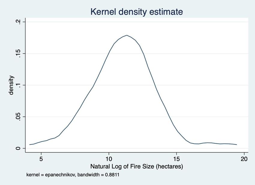
Bushfire detection

  likely changes in the distribution of fires due to climate change (obtained from the
 existing literature).
The first step is to model the likely growth through time in the number of fires that occur
under adverse fire conditions, which is done using a Poisson distribution.15 The second step is
to apply a distribution to the size and location of each of the fires. Based on observed data,
the distribution of both fire size and population density are estimated to follow independent,
log-normal distributions. The observed density functions are summarised in Figure 5 and 6
respectively, with fire size appearing to more closely approximate a normal distribution.16
Figure 5 Observed distribution of natural log of fire size

15
 We also tested for and rejected overdispersion using the negative binomial model, though it should be
 pointed out this was primarily due to quite wide confidence intervals due to the relatively small sample.
 We assume the time trend observed between 1990 and 2019 is fixed at the end of the period, giving a
 model for the Poisson distribution of the probability of the number of fires (X) in a given year (t) being
 equal to k as:
 − 
 ( = ) =
 !

 where = exp(−1.307988 + 0.0837808 ∗ ) and t = 0 in 1990 and is fixed initially at the 2019 value.
16
 For fire size, we estimate (via maximum likelihood estimation) a mean value for the distribution of
 10.76381 and a sigma of 2.202706. For density, the equivalent values are 0.9421025 and 0.923861
 respectively.

 17
The Australian National University Centre for Social Research and Methods

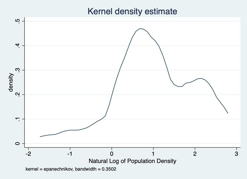
Bushfire detection

Figure 6 Observed distribution of natural log of population density of nearest urban area

The third step is to estimate the land use of the area in which the fire is located. Here, we
assume a generalised Bernoulli distribution, where the probability of being in each of the four
potential land use categories is assumed to follow the same distribution as in the observed
database.17
With the above set of assumptions, we create a synthetic dataset that has a simulated number
of fires for each year between 2020 and 2049, with a simulated size and location for each fire.18
We then apply our model for insured costs, as well as the multiplier for total costs, which gives
us an estimate of the cost of each fire.
It is standard in cost-effectiveness/cost-benefit analysis to assume that a cost or benefit
incurred or received in the future is worth less than one incurred or received in the present
year. The intuition for this is that, in terms of benefits, if that money was available now, then
it could be invested with a reasonably consistent return over the long-run. In terms of costs, a
person can invest less than the future costs now and have the funds available to cover those
costs in the future. The difference between a dollar amount now and in the future is known as
the discount rate, which we set to 4 per cent, following a House of Representatives Standing
Committee on Infrastructure, Transport and Cities recommendation.

17
 Specifically, 33.3 per cent of fires are assumed to be in ‘Conservation and Natural Environments’, 8.3 per
 cent in ‘Production from Relatively Natural Environments’, 27.8 per cent in ‘Production from Dryland
 Agriculture and Plantations’, and 30.6 per cent in ‘Intensive Uses.’
18
 In order to avoid extremes in the distributions, we restrict the number of fires to 6 in a given year (one
 more than the maximum in the observed dataset) and the fire size to 12 million hectares (roughly 20 per
 cent larger than the largest fire in the observed dataset).

 18
The Australian National University Centre for Social Research and Methods

Bushfire detection

The process described above gives us the Net Present Value for simulated bushfire costs under
the scenario of the predicted level of bushfires continuing into the future. We set up two
additional counterfactual scenarios, which factor in future additional increases in the number
of fires due to climate change (we make the conservative assumption that the size distribution
of fires is unchanged). Following Sharples, Cary et al. (2016) we assume a 30 per cent increase
in fires by 2050 as our ‘high climate change’ scenario (or a 0.88 per cent increase per year,
compounded) and a 15 per cent increase in fires by 2050 as our moderate climate change
scenario (a 0.44 per cent increase per year, compounded).
4.3 Simulated distributions of fires under early fire detection scenarios and
 calculation of cost savings from early fire detection
The counterfactual fire size and cost distributions (Section 4.2) describe the projected costs of
large bushfires (i.e. those that are present in the costs database) in the absence of any major
policy change related to fire detection or suppression, but taking into account future growth
due to climate change. The aim of this paper, and the final part of the methodology, is to
identify a set of potential treatment distributions under the scenario of reduced detection
times of fires.
We incorporate the introduction of such an early fire detection by assuming that the main
effect will be to reduce the probability of a fire entering the insurance database in the first
place due to a cost of at least $10 million (that is, the number of large fires each year), rather
than the size or costs of fires that have an insured cost of over $10 million. The intuition is that
early detection will have little impact on fire size and costs if the first attack is not successful,
but rather increase the chance of there being a successful first attack.
The main challenge in estimating the potential effect of an early detection system is that we
do not know the current distribution of fire detection times, as fire ignitions are generally not
observed. We do, however, have data from Plucinski (2012) which showed that in periods of
extreme fire danger, if the time taken between detection and arrival of first attack is less than
30 minutes, then the chance of successful suppression is estimated to be 40 per cent. We can
conceptualise a reduced detection time as being equivalent to an increased chance of arriving
at the fire within 30 minutes of ignition (what ultimately matters is time between ignition and
arrival).
Furthermore, we have information on 34 forest fires between 2005 and 2007 where the Forest
Fire Danger Index was greater than or equal to 50. On those days, the mean time between
detection and first attack is 1.45 hours, with a standard deviation of 2.80. We once again
estimate a log-normal distribution for this data.19
Using the observed distribution, 55.9 per cent of fires are responded to within 30 minutes,
which means 22.4 per cent are assumed to be successfully dealt with at first attack (based on
the success rate identified above). Under scenario one, we assume that detection time is
improved by 30 minutes. This means, using the observed distribution that 70.6 per cent are
responded to within the first 30 minutes, leading to 28.2 per cent being dealt with, or a
reduction in the number of fires that are not dealt with of 7.5 per cent.20 Under scenario two,
we assume detection time is reduced by a further 30 minutes, which based on the observed

19
 mean = -0.5622704 and sigma = 1.283504)
20 1−0.282
 (1 − ( ))
 1−0.224

 19
The Australian National University Centre for Social Research and Methods

Bushfire detection

distribution means that 88.2 per cent of fires are responded to within 30 minutes, leading to
35.3 per cent being dealt with, or a reduction in the number of fires that are not dealt with of
16.6 per cent.21 The final scenario is where early detection leads to all fires being responded
to within 30 minutes, resulting in a 40.0 success rate, or a 22.7 per cent reduction in the
number of fires compared to the counterfactual scenario.
In the treatment scenarios, we therefore, reduce the probability of each given fire occurring
by 7.47 per cent (Scenario 1), 16.6 per cent (Scenario 2) and 22.7 per cent (Scenario 3). We do
not make any assessment as to the feasibility of early detection systems achieving these
outcomes.

5 Results
Bushfires are expected to result in significant economic costs over the next thirty years (2020
to 2049) and these costs are projected to grow under the scenarios in which climate change
increases the number of fires. The modelling also shows, for a range of scenarios, that earlier
fire detection which reduces bushfire risk would have significant economic benefits. This
section first presents the results of the simulation of the number of high cost fires (over $10
million insurance cost) under the various climate change and fire detection speed scenarios. It
then presents the estimates of the costs of the economic costs of fires under the various
scenarios and the economic benefits that may result from the different scenarios related to
early fire detection.
The discussion of results begins with the simulated number of large fires per year. (Table 4).22
In the absence of any change in the speed of fire detection or changes in the frequency of fires
due to climate change, we estimate that there will be an average of 3.06 large fires per year
over the 2020 to 2049 period. Under the moderate climate change scenario (fire frequency
increases by 15 per cent) we estimate that there will be an average of 3.30 fires per year, and
under the high climate change scenario (fire frequency increase by 30 per cent) we estimate
that on average there will be 3.53 large fires per year.
Early detection of fires is estimated to reduce the number of fires per year, but not eliminate
them. Even under our most optimistic scenario that there will be no increase in fires from
climate change and that all fires will be detected in such a way as to lead to responses within
30 minutes, we are still estimating 2.39 large fires per year over the period. An example of such
fires is the 2020 Australian Capital Territory (ACT) Orroral Valley which was detected almost
instantaneously, with professional fire crews within very close proximity. However, it still led
to over 80,000 hectares being burned, an ACT State of Emergency, and has been described as
‘the territory’s worst ever environmental disaster.’23
One comparison that is worth making is between the average number of large fires in our
middle Scenario 2 (a one-hour reduction in response time) under the projected increase in

21 1−0.353
 (1 − ( ))
 1−0.224
22
 Results presented in Table 4 are based on 1,000 replications, pseudo-randomly drawing from the
 estimated distribution of fires as discussed in the previous section. A pseudo-random number generator
 uses an initial seed value (in this paper, we use 15) and an algorithm for generating a sequence of
 numbers whose properties approximate the properties of sequences of random numbers. (L'ecuyer P.
 Pseudorandom number generators. Encyclopedia of Quantitative Finance. 2010 May 15.)
23
 https://www.abc.net.au/news/2020-02-16/namadgi-national-park-recovery-after-orroral-valley-
 fire/11968950

 20
The Australian National University Centre for Social Research and Methods

Bushfire detection

fires due to climate change (2.96 fires per year) and the average number of fires with no policy
change in the absence of any climate change effects (3.06 fires per year). A very significant
increase in early detection is only likely to bring the distribution of fires back to roughly what
it would have been in the absence of climate change-related increases.
Table 4 Simulated average number of large fires per year (2020-2049)
 Detection scenarios
 Climate change scenarios No change in Scenario 1 Scenario 2 Scenario 3
 detection
 (30-min (60-min (all fires responded
 times
 reduction) reduction) to within 30-min)
 No growth 3.06 2.84 2.57 2.39
 Moderate climate change (15% growth) 3.30 3.07 2.77 2.57
 High climate change (30% growth) 3.53 3.29 2.96 2.76

Based on the modelling of economic costs we estimate that bushfires will cost, in Net Present
Value terms, between $1.1 billion per year in the absence of climate change increasing the
number of fires and $1.2 billion per year under the high climate change scenario (top panel of
Table 5). The undiscounted economic cost of fires averaged over the period 2020 to 2049 is
between $1.9 billion per year in the absence of climate change increasing the number of fires
and $2.2 billion per year under the high climate change scenario (bottom panel of Table 5).
Table 5 Simulated average cost of large fires per year (2020-2049)
 Detection scenarios
 Climate change No change in Scenario 1 Scenario 2 Scenario 3
 scenarios detection times
 (30-min reduction) (60-min reduction) (all fires responded
 to within 30-min)
 Net Present Value
 No growth $1,103,880,576 $1,017,468,160 $913,638,080 $853,655,168
 Moderate climate $1,159,702,784 $1,068,843,456 $959,046,464 $887,380,800
 change (15%
 growth)
 High climate change $1,211,963,648 $1,125,198,976 $1,012,863,360 $937,132,224
 (30% growth)
 Undiscounted values
 No growth $1,911,119,488 $1,754,565,504 $1,588,569,088 $1,477,930,496
 Moderate climate $2,038,681,472 $1,875,301,760 $1,683,185,664 $1,559,620,224
 change (15%
 growth)
 High climate change $2,156,314,112 $1,995,298,560 $1,791,100,672 $1,664,713,856
 (30% growth)

The estimated costs per year between 2020 and 2049 expressed in Net Present Value terms
are less than the estimated costs for 2009 to 2019, presented in the previous section. The
reason for this is the discounting of the costs of future fires, which is a common approach used
in studies of value for money. However, an alternative, not unreasonable assumption is that
we value the future in exactly the same way as we value the present, and the only discounting

 21
The Australian National University Centre for Social Research and Methods

Bushfire detection

that should occur is for inflation (which is held constant in our model). The effect of this is
shown across the two panels in Table 5, as well as more explicitly in Figure 7, which gives the
simulated costs of fires per year in their original value, and after discounting to Net Present
Value terms, under the scenario of 30 per cent growth of fires due to climate change and no
policy intervention. Costs increase without discounting, but decrease under discounting
(because the discount rate used by the government is far greater than the annual growth in
fires under the scenario we model).
In deciding whether to invest in early detection technology, we still recommend the use of a
discount rate as best practice, but do also recognise that different assumptions may lead to
somewhat different conclusions and provide both discounted and non-discounted values.
Figure 7 Costs of fires per year with and without discounting – 30 per cent growth over
 period/no change in detection scenario
 $3,000,000,000

 $2,500,000,000

 $2,000,000,000

 $1,500,000,000

 $1,000,000,000

 $500,000,000

 $0
 2020
 2021
 2022
 2023
 2024
 2025
 2026
 2027
 2028
 2029
 2030
 2031
 2032
 2033
 2034
 2035
 2036
 2037
 2038
 2039
 2040
 2041
 2042
 2043
 2044
 2045
 2046
 2047
 2048
 2049

 Simulat ed costs per year Discounted costs per year

So, what does that yearly reduction in costs translate to over a thirty-year period? Quite a lot.
Table 6 gives the difference in costs between the detection scenarios and the baseline
counterfactual distribution, summed over all 30 years of the simulation period. In the absence
of any increase in fires due to climate change, we estimate a reduction in the economic costs
of fires by $2.6billion, even with improvements in response times by 30 minutes. Under the
Sharples et al. (2016) climate change scenario, and with the very strong assumption of all fires
being able to be responded to within 30 minutes, we estimate a total benefit of $8.2billion, in
2019 dollars and in Net Present Value terms, or $14.8 billion in non-discounted terms.

 22
The Australian National University Centre for Social Research and Methods

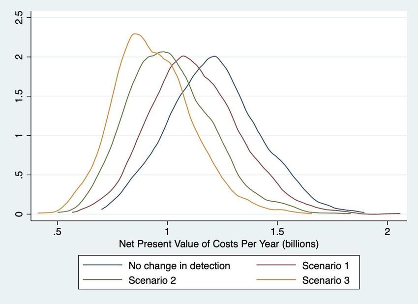
Bushfire detection

Table 6 Simulated total benefit over 30 years of earlier fire detection (2020-2049)
 Detection scenarios
 Climate change scenarios Scenario 1 Scenario 2 Scenario 3
 (30-min reduction) (60-min reduction) (all fires responded
 to within 30-min)
 Net Present Value
 No growth $2,592,372,480 $5,707,274,880 $7,506,762,240
 Moderate climate change (15% $2,725,779,840 $6,019,689,600 $8,169,659,520
 growth)
 High climate change (30% $2,602,940,160 $5,973,008,640 $8,244,942,720
 growth)
 Undiscounted values
 No growth $4,696,619,520 $9,676,512,000 $12,995,669,760
 Moderate climate change (15% $4,901,391,360 $10,664,874,240 $14,371,837,440
 growth)
 High climate change (30% $4,830,466,560 $10,956,403,200 $14,748,007,680
 growth)

It is impossible to know what the level and costs of fire activity are likely to be in a given year
into the future. Our method relies on estimating parameters for a set of observed distributions
and then randomly drawing from those distributions for each year and for each scenario. We
do this a thousand times, and then take the average across those replications as an estimate
of the likely number of fires and associated costs. However, while the average value is in many
ways the most likely outcome, it is not the only plausible outcome and any one of our
replications represents a plausible value. The distribution of those plausible values is a useful
measure of the uncertainty around the estimates of the costs of bushfires, and the benefits in
response times due to early detection.
Based on the largest increase in fires due to climate change, Figure 8 shows the estimated
distribution of costs under the counterfactual scenario, as well as under the three treatment
scenarios for early detection. Not surprisingly given the results presented in Table 5, the
greater the reduction in fire probability due to the assumed effect of early detection, the lower
the average economic cost per year from bushfires. This is represented by a shift to the left in
the distributions. However, there is also a noticeable narrowing of the distribution in Scenario
3 compared to the other three scenarios, representing a smaller standard deviation.

 23
The Australian National University Centre for Social Research and Methods