Informative Bayesian Neural Network Priors for Weak Signals
←
→
Page content transcription
If your browser does not render page correctly, please read the page content below
Bayesian Analysis (2021)                   TBA, Number TBA, pp. 1–31

Informative Bayesian Neural Network Priors for
                Weak Signals∗

      Tianyu Cui† , Aki Havulinna‡,§ , Pekka Marttinen†,‡, , and Samuel Kaski†,¶,

      Abstract. Encoding domain knowledge into the prior over the high-dimensional
      weight space of a neural network is challenging but essential in applications with
      limited data and weak signals. Two types of domain knowledge are commonly
      available in scientific applications: 1. feature sparsity (fraction of features deemed
      relevant); 2. signal-to-noise ratio, quantified, for instance, as the proportion of vari-
      ance explained. We show how to encode both types of domain knowledge into the
      widely used Gaussian scale mixture priors with Automatic Relevance Determina-
      tion. Specifically, we propose a new joint prior over the local (i.e., feature-specific)
      scale parameters that encodes knowledge about feature sparsity, and a Stein gradi-
      ent optimization to tune the hyperparameters in such a way that the distribution
      induced on the model’s proportion of variance explained matches the prior dis-
      tribution. We show empirically that the new prior improves prediction accuracy
      compared to existing neural network priors on publicly available datasets and in a
      genetics application where signals are weak and sparse, often outperforming even
      computationally intensive cross-validation for hyperparameter tuning.
      Keywords: informative prior, neural network, proportion of variance explained,
      sparsity.

1     Introduction
Neural networks (NNs) have achieved state-of-the-art performance on a wide range of
supervised learning tasks with high a signal-to-noise ratio (S/N), such as computer
vision (Krizhevsky et al., 2012) and natural language processing (Devlin et al., 2018).
However, NNs often fail in scientific applications where domain knowledge is essential,
e.g., when data are limited or the signal is extremely weak and sparse. Applications in
genetics often fall into the latter category and are used as the motivating example for
our derivations. Bayesian approach (Gelman et al., 2013) has been of interest in the NN
community because of its ability to incorporate domain knowledge into reasoning and
to provide principled handling of uncertainty. Nevertheless, it is still largely an open

   ∗ This work was supported by the Academy of Finland (Flagship programme: Finnish Center for

Artificial Intelligence, FCAI, grants 319264, 292334, 286607, 294015, 336033, 315896, 341763), and EU
Horizon 2020 (INTERVENE, grant no. 101016775). We also acknowledge the computational resources
provided by the Aalto Science-IT Project from Computer Science IT.
   † Helsinki Institute for Information Technology HIIT, Department of Computer Science, Aalto Uni-

versity, Finland, tianyu.cui@aalto.fi
   ‡ Finnish Institute for Health and Welfare (THL), Finland
   § Institute for Molecular Medicine Finland, FIMM-HiLIFE, Helsinki, Finland
   ¶ Department of Computer Science, University of Manchester, UK
    Equal contribution.


c 2021 International Society for Bayesian Analysis            https://doi.org/10.1214/21-BA1291
2 Informative Neural Network Priors
Figure 1: a) A spike-and-slab prior with slab probability p = 0.05 induces a binomial
distribution on the number of relevant features. The proposed informative spike-and-
slab can encode a spectrum of alternative beliefs, such as a discretized or ‘flattened’
Laplace (for details, see Section 3). b) The informative spike-and-slab prior can remove
false features more effectively than the vanilla spike-and-slab prior with correct slab
probability, where features are assumed independent (see Section 6.1).
question how to encode domain knowledge into the prior over Bayesian neural network
(BNN) weights, which are often high-dimensional and uninterpretable.
We study the family of Gaussian scale mixture (GSM) (Andrews and Mallows, 1974)
distributions, which are widely used as priors for BNN weights. A particular example
of interest is the spike-and-slab prior (Mitchell and Beauchamp, 1988)
(l) (l) (l) (l)2 (l)2 (l)
wij |σ, λi , τi ∼ N (0, σ (l)2 λi τi ); τi ∼ Bernoulli(p), (1)
(l)
where wij represents the NN weight from node i in layer l to node j in layer l + 1.
(l)
The hyper-parameters {σ (l) , λi , p} are often given non-informative hyper-priors (Neal,
(l)
2012), such as the inverse Gamma on σ (l) and λi , or optimized using cross-validation
(Blundell et al., 2015). In contrast, we propose determining the hyper-priors according
to two types of domain knowledge often available in scientific applications: ballpark
figures on feature sparsity and the signal-to-noise ratio. Feature sparsity refers to the
expected fraction of features used by the model. For example, it is known that less than
2% of the genome encodes for genes, which may inform the expectation on the fraction
of relevant features in a genetics application. A prior on the signal-to-noise ratio specifies
the amount of target variance expected to be explained by the chosen features, and it
can be quantified as the proportion of variance explained (PVE) (Glantz et al., 1990).
For instance, one gene may explain a tiny fraction of the variance of a given phenotype
(prediction target in genetics, e.g. the height of an individual), i.e., the PVE of a gene
may be as little as 1%.
Existing scalable sparsity-inducing BNN priors, such as the spike-and-slab prior, are
restricted in the forms of prior beliefs about sparsity they can express: conditionally
on the slab probability p the number of relevant features follows a Binomial distribu-
tion. Specifying a Beta hyper-prior on p could increase flexibility, but this still is more
restricted and less intuitive than specifying any distribution directly on the number ofT. Cui, A. Havulinna, P. Marttinen, and S. Kaski 3
Figure 2: a) The empirical distribution and corresponding kernel density estimation
(KDE) of the proportion of variance explained (PVE) for a BNN, obtained by simulating
from the model, before and after optimizing the hyperparameters according to the prior
belief on the PVE. b) The data with PVE=0.8 in its generating process are more likely
to be generated by a BNN when the mode of the PVE is approximately correctly (left)
than incorrectly (right). Colored lines are functions sampled from the BNN (for details,
see Section 4).
relevant features, and in practice in the BNN literature a point estimate for p is used.
The value of p is either set manually, cross-validated, or optimized as part of MAP
estimation (Deng et al., 2019). Moreover, the weights for different features or nodes
are (conditionally) independent in (1); thus, incorporating correct features will not help
remove false ones. In this paper, we propose a novel informative hyper-prior over the
(l)
feature inclusion indicators τi , called informative spike-and-slab, which can directly
model any distribution on the number of relevant features (Figure 1a). In addition,
(l)
unlike the vanilla spike-and-slab, the τi for different features i are dependent in the
new informative spike-and-slab, and consequently false features are more likely to be
removed when correct features are included, which can be extremely beneficial when
the noise level is high, as demonstrated with a toy example in Figure 1b.
The PVE assumed by a BNN affects the variability of functions drawn from the prior
(Figure 2b). Intuitively, when the PVE of a BNN is close to the correct PVE, the model
is more likely to recover the underlying data generating function. The distribution of
PVE assumed by a BNN is induced by the prior on the model’s weights, which in turn is
affected by all the hyper-parameters. Thus, hyper-parameters that do not affect feature
(l)
sparsity, e.g. λi , can be used to encode domain knowledge about the PVE. We propose
a scalable gradient-based optimization approach to match the model’s PVE with the
prior belief on the PVE, e.g., a Beta distribution, by minimizing the Kullback–Leibler di-
vergence between the two distributions w.r.t. chosen hyper-parameters using the Stein
gradient estimator (Li and Turner, 2018) (Figure 2a). Although it has been demon-
strated that using cross-validation to specify hyper-parameters, e.g. the global scale in
the mean-field prior, is sufficient for tasks with a high S/N and a large dataset (Wilson
and Izmailov, 2020), we empirically show that being informative about the PVE can
improve performance in low S/N and small data regimes, even without computationally
intensive cross-validation.
The structure of this paper is the following. Section 2 reviews required background on
Bayesian neural networks and Stein gradients. In Section 3, we describe our novel joint4 Informative Neural Network Priors
hyper-prior over the local scales which explicitly encodes feature sparsity. In Section 4,
we present the novel optimization algorithm to tune the distribution of a model’s PVE
according to prior knowledge. Section 5 provides the variational inference algorithm for
BNNs. Section 6 reviews in detail a large body of related literature on BNNs. Thorough
experiments with synthetic and real-world data sets are presented in Section 7, demon-
strating the benefits of the method. Finally, Section 8 concludes, including discussion
on limitations of our method as well as suggested future directions.
2 Background
2.1 Proportion of Variance Explained
In regression tasks, we assume that the data generating process takes the form
y = f (x; w) + , (2)
where f (x; w) is the unknown target function, and is the unexplainable noise. The
Proportion of Variance Explained (PVE) (Glantz et al., 1990) of f (x; w) on dataset
{X, y} with input X = {x(1) , . . . , x(N ) } and outputs y = {y (1) , . . . , y (N ) }, also called
the coefficient of determination (R2 ) in linear regression, is
N
(y (i) − f (x(i) ; w))2
PVE(w) = 1 − i=1N . (3)
(i) − ȳ)2
i=1 (y
The PVE is commonly used to measure the impact of features x on the prediction target
y, for example in genomics (Marttinen et al., 2014). In general, PVE should be in [0, 1]
because the predictions’ variance should not exceed that of the data. However, this may
not hold at test time for non-linear models such as neural networks if the models have
overfitted to the training data, in which case the variance of the residual can exceed the
variance of target in the test set. By placing a prior over w whose PVE(w) concentrates
around the PVE of the data generating process, the hypothesis space of the prior can
be made more concentrated around the true model, which eventually yields a more
accurate posterior.
2.2 Bayesian neural networks
Variational posterior approximation
Bayesian neural networks (BNNs) (MacKay, 1992; Neal, 2012) are defined by placing a
prior distribution on the weights p(w) of a NN. Then, instead of finding point estimators
of weights by minimizing a cost function, which is the normal practice in NNs, a posterior
distribution of the weights is calculated conditionally on the data. Let f (x; w) denote the
output of a BNN and p(y|x, w) = p(y|f (x; w)) the likelihood. Then, given a dataset of
inputs X = {x(1) , . . . , x(N ) } and outputs y = {y (1) , . . . , y (N ) }, training a BNN means
computing the posterior distribution p(w|X, y). Variational inference can be used to
approximate the intractable p(w|X, y) with a simpler distribution, qφ (w), by minimizingT. Cui, A. Havulinna, P. Marttinen, and S. Kaski 5
KL(qφ (w)||p(w|X, y)). This is equivalent to maximizing the Evidence Lower BOund
(ELBO) (Bishop, 2006)
L(φ) = H(qφ (w)) + Eqφ (w) [log p(y, w|X)]. (4)
The first term in (4) is the entropy of the approximated posterior, which can be cal-
culated analytically for many choices of qφ (w). The second term is often estimated
by the reparametrization trick (Kingma and Welling, 2013), which reparametrizes the
approximated posterior qφ (w) using a deterministic and differentiable transformation
w = g(ξ; φ) with ξ ∼ p(ξ), such that Eqφ (w) [log p(y, w|X)] = Ep(ξ) [log p(y, g(ξ; φ)|X)],
which can be estimated by Monte Carlo integration.
Gaussian scale mixture priors over weights
The Gaussian scale mixture (GSM) (Andrews and Mallows, 1974) is defined to be a zero
mean Gaussian conditional on its scales. In BNNs, it has been combined with Automatic
Relevance Determination (ARD) (MacKay, 1994), a widely used approach for feature
selection in non-linear models. An ARD prior in BNNs means that all of the outgoing
(l) (l)
weights wij from node i in layer l share a same scale λi (Neal, 2012). We define the
(l)
input layer as layer 0 for simplicity. A GSM ARD prior on each weight wij can be
written in a hierarchically parametrized form as follows:
(l) (l) (l)2 (l) (l)
wij |λi , σ (l) ∼ N (0, σ (l)2 λi ); λi ∼ p(λi ; θλ ), (5)
where σ (l) is the layer-wise global scale shared by all weights in layer l, which can either
(l)
be set to a constant value or estimated using non-informative priors, and p(λi ; θλ ) de-
(l)
fines a hyper-prior on the local scales. The marginal distribution of wij can be obtained
by integrating out the local scales given σ (l) :
(l) (l) (l)2 (l) (l)
p(wij |σ ) = N (0, σ (l)2 λi )p(λi ; θλ )dλi . (6)
(l) (l)
The hyper-prior of local scales p(λi ; θλ ) determines the distribution of p(wij |σ (l) ). For
(l) (l)
example, a Dirac delta distribution δ(λi − 1) reduces p(wij |σ (l) ) to a Gaussian with
(l)
mean zero and variance σ (l)2 , whereas an inverse Gamma distribution on λi makes
(l)
p(wij |σ (l) ) equal to a student-t distribution (Gelman et al., 2013; Fortuin et al., 2021).
Many sparsity inducing priors in the Bayesian paradigm can be interpreted as Gaus-
(l)
sian scale mixture priors with additional local scale variables τi :
(l) (l) (l) (l)2 (l)2 (l) (l) (l) (l)
wij |λi , τi , σ (l) ∼ N (0, σ (l)2 λi τi ); λi ∼ p(λi ; θλ ); τi ∼ p(τi ; θτ ). (7)
For example, the spike-and-slab prior (Mitchell and Beauchamp, 1988) is the ‘gold
(l)
standard’ for sparse models and it introduces binary local scales τi , interpreted as
feature inclusion indicators, such that
(l) (l) (l) (l) (l) (l) (l)2
wij |λi , τi , σ (l) ∼ (1 − τi )δ(wij ) + τi N (0, σ (l)2 λi ), (8)6 Informative Neural Network Priors
Figure 3: a) Non-centered parametrization of the GSM prior. b) The model’s PVE is
(l) (l) (l)
determined by p(λi ; θλ ) and p(τi ; θτ ) jointly, but sparsity is determined by p(τi ; θτ )
(l)
alone. Therefore, we determine the distribution p(τi ; θτ ) according to the prior knowl-
(l)
edge about sparsity, and then tune p(λi ; θλ ) conditionally on the previously selected
(l)
p(τi ; θτ ) to accommodate the prior knowledge about the PVE.
(l) (l)
where τi ∼ Bernoulli(p). In (7), the weight wij equals 0 with probability 1 − p (the
spike) and with probability p it is drawn from another Gaussian (the slab). Contin-
(l)
uous local scales τi lead to other shrinkage priors, such as the horseshoe (Piironen
and Vehtari, 2017a) and the Dirichlet-Laplace (Bhattacharya et al., 2015), which are
represented as global-local (GL) mixtures of Gaussians.
Gaussian scale mixtures, i.e., (7), are often written with an equivalent non-centered
parametrization (Papaspiliopoulos et al., 2007) (Figure 3a),
(l) (l) (l) (l) (l) (l) (l) (l) (l)
wij = σ (l) βij λi τi ; βij ∼ N (0, 1); λi ∼ p(λi ; θλ ); τi ∼ p(τi ; θτ ), (9)
which has a better posterior geometry for inference (Betancourt and Girolami, 2015)
than the hierarchical parametrization. Therefore, non-centered parametrization has been
widely used in the BNN literature (Louizos et al., 2017; Ghosh et al., 2018), and we
follow this common practice as well.
(l)
The hyper-parameter θτ in p(τi ; θτ ) controls the prior sparsity level, often quanti-
fied by the number of relevant features. However, for continuous hyper-priors, e.g. the
half-Cauchy prior in the horseshoe, which do not force weights exactly to zero, it is not
straightforward to select the hyper-parameter θτ according to prior knowledge. Piiro-
nen and Vehtari (2017b) propose to choose θτ based on the effective number of features
defined as the total shrinkage in linear regression. However, this definition relies heavily
on the linearity assumption. Thus it is non-trivial to apply on nonlinear models, such
(l)
as neural networks. On the other hand, the existing discrete hyper-priors on τi model
only restricted forms of sparsity, such as the Binomial distribution in the spike-and-slab
prior in (8). In Section 3, we propose an informative spike-and-slab prior consisting of a
(l)
new class of discrete hyper-priors over the local scales τi , capable of representing any
(l)
type of sparsity. Moreover, the informative spike-and-slab makes τi dependent, which
leads to a heavier penalization on false features than in the independent priors, such as
the vanilla spike-and-slab, after correct features have been included.T. Cui, A. Havulinna, P. Marttinen, and S. Kaski 7
It is well known that the scale parameter of the fully factorized Gaussian prior
on BNNs weights affects the variability of the functions drawn from the prior (Neal,
2012), and thus the PVE. When the PVE of the BNN has much probability around the
correct PVE, the model is more likely to recover the true data generating mechanism
(demonstration in Figure 2). As we will show in Section 4, for a BNN with the GSM prior
(l) (l)
defined in (9), the hyper-priors on the local scales, p(λi ; θλ ) and p(τi ; θτ ), control the
1
PVE jointly (Figure 3b). However, Figure 3b also shows how sparsity is determined
(l) (l)
by p(τi ; θτ ) alone. Consequently, we propose choosing p(τi ; θτ ) based on the prior
(l)
knowledge on sparsity, and after that tuning the p(λi ; θλ ) to achieve the desired level of
the PVE, such that in the end our joint prior incorporates both types of prior knowledge.
2.3 Stein Gradient Estimator
Ultimately we want to match the distribution of the PVE for a BNN prior with our prior
belief by minimizing the Kullback-Leibler divergence between these two distributions.
However, the distribution of a BNN’s PVE is analytically intractable, similarly to most
functional BNN priors. Thus the gradient of the KL-divergence is also intractable, which
makes common gradient based optimization inapplicable. Fortunately, Stein Gradient
Estimator (SGE) (Li and Turner, 2018) provides an approximation of the gradient of
the log density (i.e., ∇z log q(z)), which only requires samples from q(z) instead of its
analytical form. Central for the derivation of the SGE is the Stein’s identity (Liu et al.,
2016):
Theorem 1 (Stein’s identity). Assume that q(z) is a continuous differentiable proba-
bility density supported on Z ⊂ Rd , h : Z → Rd is a smooth vector-valued function
h(z) = [h1 (z), . . . , hd (z)]T , and h is in the Stein class of q such that
lim q(z)h(z) = 0 if Z = Rd . (10)
z→∞
Then the following identity holds:
Eq [h(z)∇z log q(z)T + ∇z h(z)] = 0. (11)
SGE estimates ∇z log q(z) by inverting (11) and approximating the expectation with
K Monte Carlo samples {z(1) , . . . , z(K) } from q(z), such that −HG ≈ K∇z h, where
K
H = (h(z(1) ), . . . , h(z(K) )) ∈ Rd ×K , ∇z h = K 1
k=1 ∇z(k) h(z
(k)
) ∈ Rd ×d , and the
matrix G = (∇z(1) log q(z(1) ), . . . , ∇z(K) log q(z(K) ))T ∈ RK×d contains the gradients of
∇z log q(z) for the K samples. Thus a ridge regression estimator is designed to estimate
G by adding an l2 regularizer:
1 η
ĜStein = arg min ∇z h + HG 2
F + G 2
F, (12)
G∈RK×d K K2
where · F is the Frobenius norm of a matrix and the penalty η ≥ 0. By solving (12),
the SGE is obtained:
ĜStein = −K(K + ηI)−1 HT ∇z h, (13)
1 The scale σ (l) is often estimated using a non-informative prior or cross-validated.8 Informative Neural Network Priors
where K = HT H is the kernel matrix, such that Kij = K(z(i) , z(j) ) = h(z(i) )T h(z(j) ),
K
and (HT ∇z h)ij = k=1 ∇z(k) K(z(i) , z(k) ), where K(·, ·) is the kernel function. It has
j
been shown that the default RBF kernel satisfies Stein’s identity, and we adopt it in
this work. In Section 4, we will use SGE to learn the hyper-parameters of the GSM
prior for BNN weights such that the resulting distribution of the PVE matches our
prior knowledge about the strength of the signal.
3 Prior knowledge about sparsity
(l)
In this section, we propose a new hyper-prior for the local scales p(τi ; θτ ) to model
prior beliefs about sparsity. The new prior generates the local scales conditionally on
the number of relevant features, which allows us to explicitly express prior knowledge
about the number of relevant features. We focus on the case where each local scale
(l)
τi is assumed to be binary with domain {0, 1}, analogously to the feature inclusion
indicators in the spike-and-slab prior.
3.1 Prior on the number of relevant features
We control sparsity by placing a prior on the number of relevant features m using a
probability mass function pm (m; θm ), where 0 ≤ m ≤ D (dimension of the dataset).
Intuitively, if pm concentrates close to 0, a sparse model with few features is preferred; if
pm places much probability mass close to D, then all of the features are likely to be used
instead. Hence, unlike other priors encouraging shrinkage, such as the horseshoe, our
new prior easily incorporates experts’ knowledge about the number of relevant features.
In practice, pm (m; θm ) is chosen based on the available prior knowledge. When there is
a good idea about the number of relevant features, a unimodal distribution, such as a
discretized Laplace, can be used:
sm |m − μm |
pm (m; μ, sm ) = cn exp − , (14)
2
where μm is the mode, sm is the precision, and cn is the normalization constant. Often
only an interval for the number of relevant features is available. Then it is possible to
use, for example, a ‘flattened’ Laplace (Figure 1):
sm R(m; μ+ , μ− )
pm (m; μ− , μ+ , sm ) = cn exp − ,
2 (15)
R(m; μ− , μ+ ) = max {(m − μ+ ), (μ− − m), 0} ,
where [μ− , μ+ ] defines the interval where the probability is uniform and reaches its
maximum value, and cn is the corresponding normalization constant. Equation 14 and 15
include the (discretized) exponential distribution as a special case with μm = 0 and
μ− = μ+ = 0 respectively; it has been widely studied in sparse deep learning literature
(Polson and Ročková, 2018; Wang and Ročková, 2020). The ‘flattened’ Laplace, with
a high precision sm , is a continuous approximation of the distribution with a uniformT. Cui, A. Havulinna, P. Marttinen, and S. Kaski 9
Figure 4: A visualization of ‘flattened’ Laplace prior with different hyper-parameters.
‘Discretized’ exponential (red) and uniform (yellow) distributions are special cases of
the ‘flattened’ Laplace.
probability mass within [μ− , μ+ ] and 0 outside of [μ− , μ+ ] (blue in Figure 4). If there
is no prior information about sparsity, a discrete uniform prior over [0, D] is a plausible
alternative. See Figure 4 for a visualization.
3.2 Feature allocation
Conditionally on the number of features m, we introduce indicators Ii ∈ {0, 1} to denote
D
if a feature i is used by the model (Ii = 1) or not (Ii = 0), such that m = i=1 Ii .
We then marginalize over m using pm (m; θm ). We assume there is no prior knowledge
about relative importance of features (this assumption can be easily relaxed if needed),
D
i.e., {Ii }i=1 has a jointly uniform distribution given m:
D
D
p({Ii }i=1 |m) = cd δ[m − Ii ], (16)
i=1
D −1
where the normalization constant is cd = m . Now we can calculate the joint distri-
D
bution of {Ii }i=1 by marginalizing out m:
D
D
D
−1
Ii ; θ m ) D
D D
p({Ii }i=1 ; θm ) = pm (m; θm )p({Ii }i=1 |m) = pm ( . (17)
m=0 i=1 i=1 Ii
(l) (l)
When the local scale variables τi are binary, the τi take the role of the identity
variables Ii . Thus we obtain a joint distribution over discrete scale parameters τi as
(l) (l)
D
D
−1
τi ; θ m ) D
(l)
p(τ1 , . . . , τD ; θτ ) = pm ( (l) , (18)
i=1 i=1 τi
where θτ represents the same set of hyper-parameters as θm , and the distribution
D (l)
pm ( i=1 τi ; θm ) models the beliefs of the number of relevant features. In general,10 Informative Neural Network Priors
(l)
the local scales {τi }D
i=1 in (18) are dependent. However, when pm (·) is set to a Bino-
(l)
mial (or its Gaussian approximation), the joint distribution of {τi }D i=1 factorizes into
a product of independent Bernoullis corresponding to the vanilla spike-and-slab with a
fixed slab probability (8). We refer to (18) as the informative spike-and-slab prior.
In BNNs, we suggest to use the informative spike-and-slab prior on the first layer to
inform the model about sparsity on the feature level. For hidden layers, we do not as-
sume prior domain knowledge, as they encode latent representations where such knowl-
edge is rare. However, an exponential prior on the number of hidden nodes could be
applied on each hidden layers to infer optimal layer sizes and perform Bayesian com-
pression (Kingma et al., 2015; Molchanov et al., 2017; Louizos et al., 2017), and it can
achieve near minimax rate of posterior concentration in sparse deep learning (Polson
and Ročková, 2018). It also may improve the current subnetwork inference (Daxberger
et al., 2020), that uses the simplest Gaussian priors without any sparsity, by improv-
ing subnetwork selection with explicit sparsity inducing priors. We leave these ideas as
promising topics for the future. Instead, in this work, we use the standard Gaussian
scale mixture priors in (5) for the hidden layers.
4 Prior knowledge on the PVE
After incorporating prior knowledge about sparsity in the new informative hyper-prior
(l)
p(τi ; θτ ), in this section we introduce an optimization approach to determine the hyper-
(l)
parameters (i.e., θλ ) of the hyper-prior for the other local scale parameters p(λi ; θλ )
in the GSM prior (9), based on domain knowledge about the PVE.
4.1 PVE for Bayesian neural networks
According to the definition of the PVE in (3), and assuming the noise has a zero mean,
the PVE for a regression model in (2) can be written as
Var() Var(f (X; w))
PVE(w) = 1 − = . (19)
Var(f (X; w)) + Var() Var(f (X; w)) + Var()
When f (x; w) is a BNN, PVE(w) has a distribution induced by the distribution on w.
We denote the variance of the unexplainable noise by σ2 . We use w(σ,θλ ,θτ ) to de-
note the BNN weights with a GSM prior (i.e., (9)) parametrized by hyper-parameters
{σ, θλ , θτ }, where σ is {σ (0) , . . . , σ (L) }. The PVE of a BNN with a GSM prior can be
written as
Var(f (X; w(σ,θλ ,θτ ) ))
PVE(w(σ,θλ ,θτ ) , σ ) = . (20)
Var(f (X; w(σ,θλ ,θτ ) )) + σ2
The noise σ and layer-wise global scales σ are usually given the same non-infor-
mative priors (Zhang and Bondell, 2018) or set to a default value (Blundell et al.,
2015). The hyper-parameter θτ is specified as described in Section 3. The remaining
hyper-parameter θλ we optimize to make the distribution of the PVE match our prior
knowledge about the PVE.T. Cui, A. Havulinna, P. Marttinen, and S. Kaski 11
4.2 Optimizing hyper-parameters according to prior PVE
Denote the available prior knowledge about the PVE by p(ρ). In practice such a prior
may be available from previous studies, and here we assume it can be encoded into
the reasonably flexible Beta distribution. If no prior information is available, a uniform
prior, i.e., Beta(1, 1), can be used. We incorporate such knowledge into the prior by
optimizing the hyper-parameter θλ such that the distribution induced by the BNN
weight prior, p(w; σ, θλ , θτ ), on the BNN model’s PVE denoted by qθλ (ρ(w)),2 is close
to p(ρ). We achieve this by minimizing the Kullback–Leibler divergence from qθλ (ρ(w))
to p(ρ) w.r.t. the hyper-parameter θλ , i.e., θλ∗ = arg minθλ KL[qθλ (ρ(w))|p(ρ)].
However, the KL divergence is not analytically tractable because the qθλ (ρ(w)) is
defined implicitly, such that we can only sample from qθλ (ρ(w)) but can not evaluate
its density. We first observe that the KL divergence can be approximated by:
qθλ (ρ(w)) q(ρ(g(ξ; θλ )))
KL[qθλ (ρ(w))|p(ρ)] = Ep(w;θλ ) log = Ep(ξ) log
p(ρ(w)) p(ρ(g(ξ; θλ )))
(21)
1
M
≈ log qθλ (ρ(g(ξ (m) ; θλ ))) − log p(ρ(g(ξ (m) ; θλ ))),
M m=1
by reparametrization and Monte Carlo integration. Here we assume that parameters,
which are optimized to match the p(ρ), of the GSM distribution p(w; θλ ) can be
reparametrized by a deterministic function w = g(ξ; θλ ) with ξ ∼ p(ξ). This includes
common distributions over scales, such as the half-Cauchy or the inverse gamma. For
non-reparametrizable distributions, such as the logistic distribution (Stefanski, 1991;
Izmailov et al., 2021), score function estimators can be used instead, but we leave this
for future work. Moreover, since PVE(w) is another deterministic function of w given
data X, we have PVE(w) = ρ(w) = ρ(g(ξ; θλ )). The expectation is approximated by
M samples from p(ξ). Then the gradient of the KL w.r.t. θλ can be calculated by:
1
M
∇θλ KL [qθλ (ρ(w))|p(ρ)] ≈ ∇θλ log qθλ (ρ(g(ξ (m) ; θλ ))) − log p(ρ(g(ξ (m) ; θλ )))
M m=1
1
M
= ∇θ ρ(g(ξ (m) ; θλ )) [∇ρ log qθλ (ρ) − ∇ρ log p(ρ)] .
M m=1 λ
(22)
The first term ∇θλ ρ(g(ξ (m) ; θλ )) can be calculated exactly with back-propagation pack-
ages, such as PyTorch. The last term, the gradient of the log density ∇ρ log p(ρ), is
tractable for a prior with a tractable density, such as the Beta distribution. However,
the derivative ∇ρ log qθλ (ρ) is generally intractable, as the distribution of the PVE of
a BNN qθλ (ρ) is implicitly defined by (20). We propose to apply SGE (Section 2.3) to
estimate ∇ρ log qθλ (ρ), which only requires samples from qθλ (ρ).
2 Hyper-parameters σ and θτ are omitted for simplicity as they are not optimized.12 Informative Neural Network Priors
Figure 5: Empirical distributions (50 samples) of the BNN’s PVE before (first col-
umn) and after optimizing hyper-parameters according to three different prior PVEs:
Beta(1,5), Beta(5,1) and Beta(1,1) (last three columns). Top: Results for mean-field
Gaussian prior, where the local scale is optimized. Bottom: Results for hierarchical
Gaussian prior, where the hyper-parameter of the inverse gamma prior is optimized.
When noise σ and layer-wise global scales σ are given non-informative priors, e.g.,
Inv-Gamma(0.001, 0.001), drawing samples directly according to (20) is unstable, be-
cause the variance of the non-informative prior does not exist. Fortunately, if all ac-
tivation functions of the BNN are positively homogeneous (e.g., ReLU), we have the
following theorem (proof is given in Supplementary (Cui et al., 2021)):
Theorem 2. Assume that a BNN has L layers with the Gaussian scale mixture prior in
the form of (9) and all activation functions positively homogeneous, e.g., ReLU. Then:
L
Var(f (X; w(σ,θλ ,θτ ) )) = Var(f (X; w(1,θλ ,θτ ) )) σ (l)2 . (23)
l=0
Now instead of giving non-informative priors to all layer-wise global scales, i.e.,
σ = σ (0) = . . . = σ (L) ∼ Inv-Gamma(0.001, 0.001), we propose to use σ (0) = . . . =
σ (L−1) = 1, and σ = σ (L) ∼ Inv-Gamma(0.001, 0.001). By substituting (23) with these
specifications into (20), we can write the PVE as
Var(f (X; w(1,θλ ,θτ ) )) Var(f (X; w(1,θλ ,θτ ) ))
PVE(w(σ,θλ ,θτ ) , σ ) = σ2
= , (24)
Var(f (X; w(1,θλ ,θτ ) )) + Var(f (X; w(1,θλ ,θτ ) )) + 1
σ (L)2
where the non-informative inverse Gamma distribution has canceled out, avoiding sam-
pling from it.
In practice, we find that using the whole training set, its subset, or even a simulated
dataset with a distribution similar to the test set to compute the PVE yields similar
results. Moreover, we observe that the learned hyper-parameters are not sensitive toT. Cui, A. Havulinna, P. Marttinen, and S. Kaski 13
the number of samples of SGE. This is because the distribution of the BNN’s PVE is
relatively simple and usually unimodal (e.g., Figure 5), and it depends only on a small
number of trainable hyper-parameters (see Supplementary for more details). Figure 5
illustrates the proposed approach, where we applied the method on two 3-layer BNNs
containing 100-50-30-1 nodes and the ReLU activation. We considered two GSM ARD
priors for the BNN weights: a mean-field Gaussian prior
(l) (l) (l)2 (l)
wij |λi ∼ N (0, σ (l)2 λi ); λi = σλ , (25)
and a hierarchical Gaussian prior
(l) (l) (l)2 (l)
wij |λi ∼ N (0, σ (l)2 λi ); λi ∼ Inv-Gamma(α, β), (26)
with the non-informative prior on the noise and the last layer-wise global scale. For the
Gaussian prior, it can be reparametrized by
(l) (l) (l)
wij = σλ σ (l) ξij ; ξij ∼ N (0, 1), (27)
and we optimized σλ according to the prior PVE. For the hierarchical Gaussian prior, we
optimized β while fixing α = 2 because the shape parameter of the Gamma distribution
is non-reparametrizable, and we use the following reparametrization
(l) (l) (l) (l) (l)
wij = βσ (l) ξij ηi ; ξij ∼ N (0, 1); ηi ∼ Inv-Gamma(2, 1). (28)
From Figure 5, we see that after optimizing the hyperpriors, the simulated empirical
distributions of the PVE are close to the corresponding prior knowledge in both cases,
especially when the prior knowledge is informative, such as the Beta(1, 5) or Beta(5, 1).
Moreover, we observe that even when we have fixed the shape parameter α of the inverse
Gamma, the prior is still flexible enough to approximate the prior PVE well. We provide
the whole algorithm of learning hyper-parameters in the Supplementary.
5 Learning BNNs with variational inference
We use variational inference to approximate the posterior distribution with the new
informative priors. Sampling algorithms, such as MCMC, are known to be computa-
tionally expensive for spike-and-slab priors especially with high-dimensional datasets.
According to (4), the ELBO of VI can be rewritten as,
L(φ) = Eqφ (w,σ ) [log p(y|X, w, σ )] − KL[qφ (w, σ )|p(w, σ )], (29)
where the first term is the expected log-likelihood and the second term is the Kullback–
Leibler divergence from the approximate posterior to the prior. For regression problems
studied in this work, we use the Gaussian likelihood,
p(y|X, w, σ ) = N (y; f (X; w), σ2 ), (30)14 Informative Neural Network Priors
Random variables in BNNs Prior Variational posterior
(l)
βij N (0, 1) N (μ, σ)
(l)
σ , σ (l) , λi Inv-Gamma(α, β) Log-Normal(μ, σ)
(l)
τi Bernoulli(p), Info(θτ ) Con-Bern(p)
Table 1: Variational posteriors for GSM prior. Info represents the informative spike-and-
slab prior defined in Equation 18, and Con-Bern is the concrete Bernoulli distribution
originally proposed by Maddison et al. (2016).
by assuming the unexplainable noise belongs to N (0, σ2 ). For priors in (7), we use a
fully factorized variational distribution family to approximate posteriors such that
(l)
q(w, σ ; φ) = q(σ ; φσ ) q(wij ; φw(l) )
ij
i,j,l
(l)
(l) (l)
(31)
=q(σ ; φσ ) q(βij |φβ (l) ) q(λi |φλ(l) )q(τi |φτ (l) ) q(σ (l) |φσ(l) ),
ij i i
i,j,l i,l l
according to the non-centered parametrization in (9). The explicit form of each varia-
tional posterior depends on the corresponding prior, as shown in Table 1.
Now we have defined everything required for calculating the ELBO in (29). To op-
timize the ELBO, we apply the reparametrization trick (Kingma and Welling, 2013) to
make the sampling process of the expected log-likelihood differentiable, and we com-
pute the KL divergence analytically (except for the informative prior, Info, where
reparametrization trick is used). The variational parameters are updated with Adam
(Kingma and Ba, 2014). We give the full algorithm in the Supplementary.
6 Related literature
Priors on the number of relevant features have been applied on small datasets to
induce sparsity in shallow models, e.g. NNs with one hidden layer (Vehtari, 2001), includ-
ing the geometric (Insua and Müller, 1998) and truncated Poisson (Denison et al., 1998;
Insua and Müller, 1998; Andrieu et al., 2000; Kohn et al., 2001) distributions. However,
those approaches rely on the reversible jump Markov chain Monte Carlo (RJMCMC)
to approximate the posterior (Phillips and Smith, 1996; Sykacek, 2000; Andrieu et al.,
2013), which does not scale up to deep architectures and large datasets. In this work,
we incorporate such prior beliefs into the hyper-prior on the local scales of the Gaus-
sian scale mixture prior; thus, the posterior can be approximated effectively by modern
stochastic variational inference (Hoffman et al., 2013), even for deep NN architectures
and large datasets.
Priors on PVE have been proposed to fine-tune hyper-parameters (Zhang and Bon-
dell, 2018) and to construct shrinkage priors (Zhang et al., 2020) for Bayesian linear
regression, where the distribution on the model PVE is analytically tractable. Sim-
ulation and grid search has been used to incorporate prior knowledge about a pointT. Cui, A. Havulinna, P. Marttinen, and S. Kaski 15 estimate for the PVE in Bayesian reduced rank regression (Marttinen et al., 2014), and the prediction variance in BNN with a Gaussian prior (Wilson and Izmailov, 2020). In the Supplementary, we develop a novel Monte Carlo approach to model the log-linear relationship between the global scale of the Mean-Field Gaussian prior and the predic- tion variance of the BNN to avoid computationally expensive grid search, and we use this to set the variance according to a point estimate of the PVE, but we find that the resulting nonhierarchical Gaussian prior is not flexible enough. Priors on the BNNs weights BNNs with a fully factorized Gaussian prior were pro- posed by Graves (2011) and Blundell et al. (2015). They can be interpreted as NNs with dropout by using a mixture of Dirac-delta distributions to approximate the pos- terior (Gal and Ghahramani, 2016). Nalisnick et al. (2019) extended these works and showed that NNs with any multiplicative noise could be interpreted as BNNs with GSM ARD priors. Priors over weights with low-rank assumptions, such as the k-tied normal (Swiatkowski et al., 2020) and rank-1 perturbation (Dusenberry et al., 2020) were found to have better convergence rates and ability to capture multiple modes when combined with ensemble methods. Matrix-variate Gaussian priors were proposed by Neklyudov et al. (2017) and Sun et al. (2017) to improve the expressiveness of the prior by ac- counting for the correlations between the weights. Some priors have been proposed to induce sparsity, such as the log-uniform (Molchanov et al., 2017; Louizos et al., 2017), log-normal (Neklyudov et al., 2017), horseshoe (Louizos et al., 2017; Ghosh et al., 2018), and spike-and-slab priors (Deng et al., 2019). Fortuin (2021) provided a comprehensive review about priors in Bayesian deep learning. However, none of the works can explicitly encode domain knowledge into the prior on the NN weights. Informative priors of BNNs Building of informative priors for NNs has been studied in the function space. One common type of prior information concerns the behavior of the output with certain inputs. Noise contrastive priors (NCPs) (Hafner et al., 2018) were designed to encourage reliable high uncertainty for OOD (out-of distribution) data points. Gaussian processes were proposed as a way of defining functional priors because of their ability to encode rich functional structures. Flam-Shepherd et al. (2017) trans- formed a functional GP prior into a weight-space BNN prior, with which variational inference was performed. Functional BNNs (Sun et al., 2019) perform variational in- ference directly in the functional space, where meaningful functional GP priors can be specified. Pearce et al. (2019) used a combination of different BNN architectures to encode prior knowledge about the function. Although functional priors avoid working with uninterpretable high-dimensional weights, encoding sparsity of features into the functional space is non-trivial. 7 Experiments In this section, we first compare the proposed informative sparse prior with alternatives in a feature selection task on synthetic toy data sets. We then apply it on seven public
16                                                   Informative Neural Network Priors

             Name            p(λi )                  p(τi )4                  Hyper-prior
            BetaSS     vague Inv-Gamma            Bernoulli(p)              p ∼ Beta(2, 38)
           DeltaSS     vague Inv-Gamma            Bernoulli(p)                 p = 0.05
            InfoSS     vague Inv-Gamma             FL(0, 30, 5)                  NA
              HS           C + (0, 1)          τ ∼ C + (0, ( n−p
                                                              p0
                                                                 0
                                                                   )2 )          NA
Table 2: Details of the four Gaussian scale mixture priors included in the comparison
on the synthetic datasets. The vague Inv-Gamma represents a diffuse inverse gamma
prior Inv-Gamma(0.001,0.001). FL denotes the ‘flattened’ Laplace prior defined in the
main text. NA means that the model is defined without the corresponding hyperprior.

UCI real-world datasets,3 where we tune the level of noise and the fraction of informative
features. Next, we incorporate prior knowledge about PVE into a Bayesian Wavenet
prior to evaluate its effectiveness in large-scale time series prediction tasks. Finally, in
a genetics application we show that incorporating domain knowledge on both sparsity
and the PVE can improve results in a realistic scenario.

7.1      Synthetic data
Setup We first validate the performance of the informative spike-and-slab prior pro-
posed in Section 3 on a feature selection task, using synthetic datasets similar to those
discussed by Van Der Pas et al. (2014) and Piironen and Vehtari (2017b). Instead of
a BNN, we here use linear regression, i.e., a NN without hidden layers, which enables
comparing the proposed strategy of encouraging sparsity with existing alternatives.
     Consider n datapoints generated by:

                         yi = wi + i ,   i ∼ N (0, σ2 ),   i = 1, . . . , n,               (32)

where each observation yi is obtained by adding Gaussian noise with variance σ2 to
the signal wi . We set the number of datapoints n to 400, the first p0 = 20 signals
{wi |i = 1, . . . , 20} equal to A (signal levels), and the rest of the signals to 0. We consider
3 different noise levels σ ∈ {1, 1.5, 2}, and 10 different signal levels A ∈ {1, 2, . . . , 10}.
For each parameter setting (30 in all), we generate 100 data realizations. The model
in (32) can be considered a linear regression: y = X ŵT + , where X = I and ŵ =
(A, . . . , A, 0, 0, . . . , 0) with the first p0 elements being A, so this is a feature selection
task where the number of features and datapoints are equal. We use the mean squared
error (MSE) between the posterior mean signal w̄ and the true signal ŵ to measure the
performance.

Parameter settings For estimation we use linear regression with the correct structure.
We consider 4 different Gaussian scale mixture priors on w that all follow the general
form
                wi ∼ N (0, σ 2 λ2i τi2 ); σ = 1; λi ∼ p(λi ); τi ∼ p(τi ).        (33)

     3 https://archive.ics.uci.edu/ml/index.php.
T. Cui, A. Havulinna, P. Marttinen, and S. Kaski 17
Figure 6: Synthetic datasets: A detailed visualization of the features selected by the
four priors with noise level σ = 2 and signal level A = 6 (first two columns). Results
for the two best models (DeltaSS and InfoSS) are additionally shown with a larger
signal A = 10 (the last column). Beta spike-and-slab (BetaSS) is slightly worse than
Delta spike-and-slab (DeltaSS), because the latter uses the correct slab probability.
Informative spike-and-slab (InfoSS) outperforms alternatives by making the signals
dependent. Horseshoe (HS) with the correct sparsity level overfits to the noise.
For all the spike-and-slab (SS) priors, we place a diffuse inverse Gamma prior on p(λi ).
For the BetaSS and DeltaSS priors, we assume that p(τi ) = Bernoulli(p), and define
p ∼ Beta(2, 38) for BetaSS and p = 0.05 for DeltaSS, which both reflect the correct level
of sparsity. For the informative spike-and-slab, InfoSS, we use the ‘flattened’ Laplace
(FL) prior defined in (15) with μ− = 0, μ+ = 30, and sm = 5, to encode prior knowledge
that the number of non-zero signals is (approximately) uniform on [0, 30]. We place an
p0
informative half-Cauchy prior C + (0, τ02 ) on the global shrinkage scale τ with τ0 = n−p 0
in the horseshoe (HS) (Piironen and Vehtari, 2017b), to assume the same sparsity level
as the other priors.5 The details of the different priors are shown in Table 2.
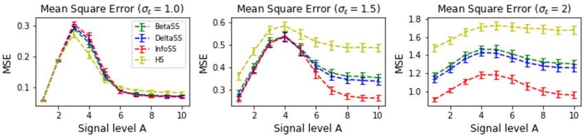
Results Figures 6 and 7 show the results on synthetic datasets. Figure 6 provides
detailed visualizations of results for the four priors with two representative signal levels
A = 6 and A = 10 and with noise level σ = 2. Figure 7 summarizes the results for
all the signal and noise levels. We first observe that the relationship between MSE and
signal level is not monotonic, which is consistent with previous studies (Piironen and
Vehtari, 2017b). Intuitively, when true signals are extremely weak, models can shrink
all signals to 0 to make the error between estimated and the true signals small, and
when the signals are strong, models can identify the true signals easily. We see that
BetaSS with p ∼ Beta(2, 38) and DeltaSS with p = 0.05 perform similarly when the
5 The effective number of features (Piironen and Vehtari, 2017b) is set to 20.18 Informative Neural Network Priors
Figure 7: Synthetic datasets: Mean squared error (MSE) between the estimated and
true signals. The bars represent the 95% confidence intervals over 100 datasets. The
novel InfoSS prior is indistinguishable from the other SS priors when for the noise level
is low. However, InfoSS is significantly more accurate than the other priors when there
is more noise.
noise level is low, but DeltaSS is better than BetaSS for higher noise levels. This is
because the DeltaSS prior is more concentrated close to the true sparsity level; thus,
it penalizes false signals more strongly (Top left and bottom panels in Figure 6). The
InfoSS prior has indistinguishable performance from the other SS priors when the noise
level is low, but with high noise, e.g., σ = 2.0, InfoSS is significantly better, especially
when the signal is large (A > 6). This is because InfoSS places a prior on the number
of features directly, which makes the signals wi dependent, and consequently including
correct signals can help remove incorrect signals. In contrast, the signals are independent
of each other in the other priors considered; thus, selecting true signals will not help
remove false findings. Another observation is that the Horseshoe prior (HS) works well
when there is little noise (e.g. σ = 1), but for larger value of σ HS is much worse than
all the spike-and-slab alternatives because it can easily overfit the noise (bottom-left
panel in Figure 6).
7.2 Public real-world UCI datasets
Setup We analyze 7 publicly available datasets:6 Bike sharing, California housing
prices, Energy efficiency, Concrete compressive strength, Yacht hydrodynamics, Boston
housing, and kin8nm dataset, whose characteristics, the number of individuals N and
the number of features D, are given in Table 4. We carry out two types of experiments:
Original datasets: we analyze the datasets as such, in which case there is no domain
knowledge about sparsity; Extended datasets: we concatenate 100 irrelevant features
with the original features and add Gaussian noise to the dependent variable such that
the PVE in the data is at most 0.2, which allows us to specify informative priors about
sparsity (the number of relevant features is at most the number of original features)
and the PVE (less than 0.2). We examine whether the performance can be improved
by encoding this extra knowledge into the prior. We use 80% of data for training and
20% for testing. We use the MSE and PVE7 (i.e., R2 ) on a test set to evaluate the
6 https://archive.ics.uci.edu/ml/index.php.
7 This is also consistent with the Mean Squared Error (MSE) when the residuals have zero mean.T. Cui, A. Havulinna, P. Marttinen, and S. Kaski 19
(l) (0) (l)
Name of the prior p(λi ), ∀l ≥ 0 p(τi ) p(τi ), ∀l ≥ 1
(l)
MF+CV λi = σλ NA NA
(l)
SS+CV λi = σλ Bernoulli(p) Bernoulli(p)
HS C + (0, 1) p(τ (0) ) = C + (0, 10−5 ) p(τ (l) ) = C + (0, 10−5 )
HMF vague Inv-Gamma NA NA
InfoHMF vague Inv-Gamma FL(0, D, 1) NA
HMF+PVE Inv-Gamma(2, β) NA NA
InfoHMF+PVE Inv-Gamma(2, β) FL(0, D, 1) NA
Table 3: Seven Gaussian scale mixture priors included in the comparison on the UCI
datasets. Hyper-parameters in MF+CV and SS+CV (local scale σλ and spike probability
p) are chosen via 5-fold cross-validation. The hyper-parameter β is optimized to match
the prior PVE, and μ+ is equal to the number of features in the corresponding original
dataset without the artificially added irrelevant features.
performance. We repeat each experiment 30 times to obtain confidence intervals, and
we give implementation details in the Supplementary. In the Supplementary, we also
provide further ablation analyses to separate the effects of two methodological novelties
by creating extended datasets with irrelevant features only and with noisy dependent
variable only. We also provide sensitivity analyses of each prior to its hyper-parameters
on ablation datasets.
Parameter settings We considered 7 different priors: 1. mean-field (independent)
Gaussian prior with cross-validation (MF+CV) (Blundell et al., 2015); 2. delta spike-
and-slab prior with cross-validation (SS+CV) (Blundell et al., 2015); 3. horseshoe prior
(HS) (Ghosh and Doshi-Velez, 2017); 4. Hierarchical Gaussian prior (HMF), which is the
same as MF+CV except that the hyperparameters receive a fully Bayesian treatment in-
stead of cross-validation. 5. The InfoHMF, which incorporates domain knowledge on
feature sparsity in the HMF by applying the proposed informative prior in the input
layer; 6. HMF+PVE instead includes the informative prior on the PVE, and finally, 7.
InfoHMF+PVE includes both types of domain knowledge. Lasso regression (Tibshirani,
2011) with cross-validated regularization (Lasso+CV) and functional Gaussian processes
prior (GP) (Sun et al., 2019) with the RBF kernel are included as other standard base-
lines.
The hyper-parameters for MF+CV priors and SS+CV prior are chosen by 5-fold cross-
validation on the training set from grids σλ ∈ {e−2 , e−1 , 1, e1 , e2 } and p ∈ {0.1, 0.3, 0.5,
0.7, 0.9}, which are wider than used in the original work by Blundell et al. (2015). We
(l)
define HS as suggested by Ghosh et al. (2018), such that the scale τi = τ (l) is shared by
all weights in each layer l. In the HMF, we use a non-informative prior on the local scales
(l)
λi . For GP, we use the hyper-parameters in the original implementation. We regard GP,
MF+CV, SS+CV, HS, and HMF as strong benchmarks to compare our novel informative priors
against. For InfoHMF, we use the ‘flattened’ Laplace (FL) prior with μ− = 0, μ+ = D
(D is the number of features in the original dataset) on the input layer to encode the
prior knowledge about feature sparsity. For HMF+PVE and InfoHMF+PVE, we optimize the20 Informative Neural Network Priors
hyper-parameter β to match the PVE of the BNN with a Beta(5.0, 1.2) for the original
datasets (the mode equals 0.95), and with Beta(1.5, 3.0) for the extended datasets (the
mode equals 0.20). For all priors that are not informative about the PVE (except the
HS), we use an Inv-Gamma(0.001,0.001) for the all layer-wise global scales σ and the
noise σ . For priors informative on the PVE, the non-informative prior is used only for
the last layer-wise global scale σ (L) and noise σ (see Section 4). The details about each
prior are summarized in Table 3.
Results The results, in terms of MSE (see test PVE in Supplementary), are reported
in Table 4. For the original datasets, we see that incorporating the prior knowledge on
the PVE (HMF+PVE and InfoHMF+PVE) always yields at least as good performance as
the corresponding prior without this knowledge (HMF and InfoHMF). Indeed, HMF+PVE
has the (shared) highest accuracy in all datasets except Boston. The new proposed in-
formative sparsity inducing prior (InfoHMF) does not here improve the performance, as
we do not have prior knowledge on sparsity in the original datasets. Among the non-
informative priors, HMF is slightly better than the rest, except for the Boston housing
dataset, where the horseshoe prior (HS) achieves the highest test PVE, which demon-
strates the benefit of the fully Bayesian treatment vs. cross-validation of the hyperpa-
rameters. Inference with the functional GP prior is computationally expensive because
the complexity of the spectral Stein gradient estimator is cubic to the number of func-
tions. Thus only a small number of functions can be used for large regression tasks such
as Bike, which harms the performance. On small datasets, e.g., Concrete, the GP prior
has competitive performance. The linear method, Lasso+CV, is worse than all BNNs in
most datasets.
In the extended datasets with the 100 extra irrelevant features and noise added
to the target, knowledge on both the PVE and sparsity improves performance signif-
icantly. For most of the datasets both types of prior knowledge are useful, and con-
sequently InfoHMF+PVE is the most accurate on 4 out of 7 datasets. Furthermore, its
PVE is also close to 20% of the maximum test PVE in the corresponding original
dataset, reflecting the fact that noise was injected to keep only 20% of the signal
(see Supplementary). We find that the horseshoe (HS) works better than the HMF on
small datasets, especially Boston, where the HS outperform others. The priors MF+CV
and SS+CV do not work well for the extended datasets, and they are even worse than
Lasso+CV, because cross-validation has a large variance on the noisy datasets espe-
cially for flexible models such as BNNs. The more computationally intensive repeated
cross-validation (Kuhn and Johnson, 2013) might alleviate the problem, but its fur-
ther exploration is left for future work. The GP priors fail to capture any signal in
extended datasets, because they do not induce any sparsity in the feature space, which
might be possible to improve with an ARD prior on the kernel. Overall, we conclude
that by incorporating knowledge on the PVE and sparsity into the prior the perfor-
mance can be improved; however, the amount of improvement can be small if the
dataset is large (California and Bike) or when the prior knowledge is weak (the original
datasets).
9 The dimension P = D in the original datasets, while P = 100 + D in the extended datasets.T. Cui, A. Havulinna, P. Marttinen, and S. Kaski 21
Original California Bike Concrete Energy Kin8nm Yacht Boston
(P, N) (9, 20k) (13, 17k) (8, 1k) (8, 0.7k) (8, 8.1k) (6, 0.3k) (3, 0.5k)
Lasso+CV 0.378 0.589 0.446 0.112 0.594 0.338 0.449
0.314 0.169 0.124 0.035 0.167 0.176 0.261
GP
(0.001) ( 0.000) (0.001) (0.001) (0.001) (0.003) (0.000)
0.220 0.067 0.193 0.185 0.087 0.049 0.216
MF+CV
(0.001) (0.000) (0.003) (0.001) (0.001) (0.001) (0.001)
0.221 0.074 0.154 0.110 0.095 0.111 0.198
SS+CV
(0.001) (0.001) (0.002) (0.000) (0.001) (0.005) (0.000)
0.215 0.073 0.172 0.106 0.097 0.078 0.190
HS
(0.001) (0.000) (0.004) (0.002) (0.001) (0.004) (0.002)
0.211 0.067 0.128 0.042 0.072 0.014 0.204
HMF
(0.002) (0.001) (0.003) (0.005) (0.001) (0.002) (0.002)
HMF 0.208 0.065 0.124 0.034 0.071 0.014 0.202
+PVE (0.002) (0.001) (0.003) (0.001) (0.001) (0.001) (0.003)
0.211 0.066 0.130 0.045 0.072 0.023 0.201
InfoHMF
(0.002) (0.001) (0.003) (0.001) (0.001) (0.001) (0.002)
InfoHMF 0.207 0.066 0.125 0.041 0.072 0.017 0.198
+PVE (0.002) (0.001) (0.002) (0.002) (0.001) (0.002) (0.002)
Extended California Bike Concrete Energy Kin8nm Yacht Boston
(P, N) (109, 20k) (113, 17k) (108, 1k) (108, 0.7k) (108, 8.1k) (106, 0.3k) (103, 0.5k)
Lasso+CV 0.867 0.913 0.956 0.854 0.899 0.893 0.985
1.002 0.998 1.006 1.004 1.001 1.040 0.983
GP
(0.002) ( 0.002) (0.008) 0.009 (0.003) (0.015) (0.000)
0.947 1.048 1.0652 0.976 1.014 1.049 1.016
MF+CV
(0.006) (0.011) (0.028) (0.039) (0.009) (0.063) (0.049)
0.878 0.911 1.0652 0.969 0.926 1.048 1.014
SS+CV
(0.006) (0.010) (0.029) (0.038) (0.008) (0.062) (0.048)
0.972 1.017 0.914 0.850 0.883 0.888 0.910
HS
(0.008) (0.010) (0.032) (0.035) (0.012) (0.054) (0.048)
0.866 0.850 0.940 0.849 0.872 0.989 0.966
HMF
(0.006) (0.008) (0.039) (0.018) (0.008) (0.059) (0.047)
HMF 0.864 0.850 0.937 0.838 0.865 0.914 0.957
+PVE (0.006) (0.008) (0.030) (0.018) (0.010) (0.072) (0.046)
0.864 0.836 0.939 0.862 0.856 0.903 0.961
InfoHMF
(0.007) (0.006) (0.021) (0.030) (0.010) (0.076) (0.039)
InfoHMF 0.861 0.827 0.927 0.841 0.846 0.886 0.914
+PVE (0.006) (0.005) (0.036) (0.018) (0.010) (0.061) (0.035)
Table 4: MSE with 1.96 standard error of the mean (in parentheses) for each prior on
UCI datasets. The first seven rows show the experimental results on the original datasets
where we have no prior information, and the last seven rows on extended datasets with
100 irrelevant features and injected noise added. The best result in each column has
been boldfaced. The dimension (P )9 and size (N ) are shown for each dataset. We see
that both information about sparsity and PVE improve the performance, especially
when prior information is available (on extended datasets).You can also read