Temporal Fusion Transformers for Interpretable Multi-horizon Time Series Forecasting
←
→
Page content transcription
If your browser does not render page correctly, please read the page content below
Temporal Fusion Transformers
                                           for Interpretable Multi-horizon Time Series Forecasting

                                                   Bryan Lima,1,∗, Sercan Ö. Arıkb , Nicolas Loeffb , Tomas Pfisterb
                                                                            a University  of Oxford, UK
                                                                             b Google   Cloud AI, USA
arXiv:1912.09363v3 [stat.ML] 27 Sep 2020

                                           Abstract
                                           Multi-horizon forecasting often contains a complex mix of inputs – including
                                           static (i.e. time-invariant) covariates, known future inputs, and other exogenous
                                           time series that are only observed in the past – without any prior information
                                           on how they interact with the target. Several deep learning methods have been
                                           proposed, but they are typically ‘black-box’ models which do not shed light on
                                           how they use the full range of inputs present in practical scenarios. In this pa-
                                           per, we introduce the Temporal Fusion Transformer (TFT) – a novel attention-
                                           based architecture which combines high-performance multi-horizon forecasting
                                           with interpretable insights into temporal dynamics. To learn temporal rela-
                                           tionships at different scales, TFT uses recurrent layers for local processing and
                                           interpretable self-attention layers for long-term dependencies. TFT utilizes spe-
                                           cialized components to select relevant features and a series of gating layers to
                                           suppress unnecessary components, enabling high performance in a wide range of
                                           scenarios. On a variety of real-world datasets, we demonstrate significant per-
                                           formance improvements over existing benchmarks, and showcase three practical
                                           interpretability use cases of TFT.
                                           Keywords: Deep learning, Interpretability, Time series, Multi-horizon
                                           forecasting, Attention mechanisms, Explainable AI.

                                           1. Introduction

                                               Multi-horizon forecasting, i.e. the prediction of variables-of-interest at mul-
                                           tiple future time steps, is a crucial problem within time series machine learning.
                                           In contrast to one-step-ahead predictions, multi-horizon forecasts provide users
                                           with access to estimates across the entire path, allowing them to optimize their
                                           actions at multiple steps in future (e.g. retailers optimizing the inventory for

                                             ∗ Corresponding  authors
                                                Email addresses: blim@robots.ox.ac.uk (Bryan Lim), soarik@google.com (Sercan Ö.
                                           Arık), nloeff@google.com (Nicolas Loeff), tpfister@google.com (Tomas Pfister)
                                              1 Completed as part of internship with Google Cloud AI Research.

                                           Preprint submitted to Elsevier                                      September 29, 2020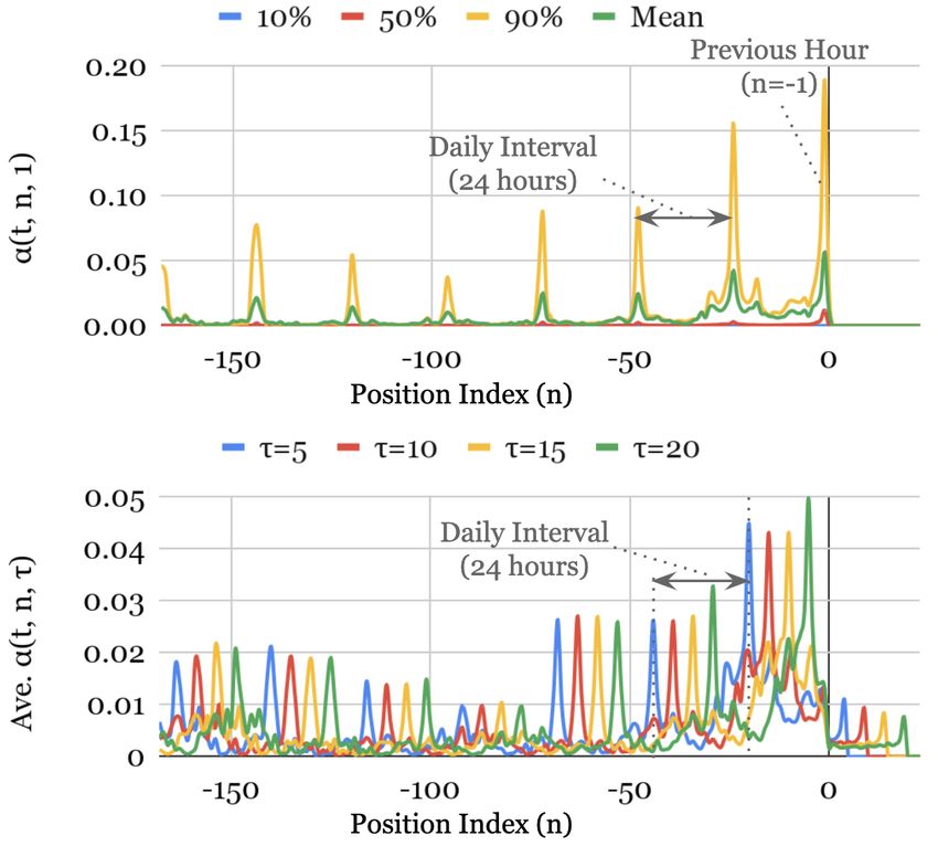
the entire upcoming season, or clinicians optimizing a treatment plan for a pa-
tient). Multi-horizon forecasting has many impactful real-world applications in
retail [1, 2], healthcare [3, 4] and economics [5]) – performance improvements
to existing methods in such applications are highly valuable.

Figure 1: Illustration of multi-horizon forecasting with static covariates, past-observed and
apriori-known future time-dependent inputs.

    Practical multi-horizon forecasting applications commonly have access to
a variety of data sources, as shown in Fig. 1, including known information
about the future (e.g. upcoming holiday dates), other exogenous time series
(e.g. historical customer foot traffic), and static metadata (e.g. location of the
store) – without any prior knowledge on how they interact. This heterogeneity
of data sources together with little information about their interactions makes
multi-horizon time series forecasting particularly challenging.
    Deep neural networks (DNNs) have increasingly been used in multi-horizon
forecasting, demonstrating strong performance improvements over traditional
time series models [6, 7, 8]. While many architectures have focused on variants
of recurrent neural network (RNN) architectures [9, 6, 10], recent improvements
have also used attention-based methods to enhance the selection of relevant time
steps in the past [11] – including Transformer-based models [12]. However, these
often fail to consider the different types of inputs commonly present in multi-
horizon forecasting, and either assume that all exogenous inputs are known
into the future [9, 6, 12] – a common problem with autoregressive models – or
neglect important static covariates [10] – which are simply concatenated with
other time-dependent features at each step. Many recent improvements in time
series models have resulted from the alignment of architectures with unique data
characteristics [13, 14]. We argue and demonstrate that similar performance
gains can also be reaped by designing networks with suitable inductive biases
for multi-horizon forecasting.
    In addition to not considering the heterogeneity of common multi-horizon
forecasting inputs, most current architectures are ‘black-box’ models where fore-

                                             2
casts are controlled by complex nonlinear interactions between many parame-
ters. This makes it difficult to explain how models arrive at their predictions,
and in turn makes it challenging for users to trust a model’s outputs and model
builders to debug it. Unfortunately, commonly-used explainability methods for
DNNs are not well-suited for applying to time series. In their conventional
form, post-hoc methods (e.g. LIME [15] and SHAP [16]) do not consider the
time ordering of input features. For example, for LIME, surrogate models are
independently constructed for each data-point, and for SHAP, features are con-
sidered independently for neighboring time steps. Such post-hoc approaches
would lead to poor explanation quality as dependencies between time steps are
typically significant in time series. On the other hand, some attention-based
architectures are proposed with inherent interpretability for sequential data,
primarily language or speech – such as the Transformer architecture [17]. The
fundamental caveat to apply them is that multi-horizon forecasting includes
many different types of input features, as opposed to language or speech. In
their conventional form, these architectures can provide insights into relevant
time steps for multi-horizon forecasting, but they cannot distinguish the impor-
tance of different features at a given timestep. Overall, in addition to the need
for new methods to tackle the heterogeneity of data in multi-horizon forecasting
for high performance, new methods are also needed to render these forecasts
interpretable, given the needs of the use cases.
    In this paper we propose the Temporal Fusion Transformer (TFT) – an
attention-based DNN architecture for multi-horizon forecasting that achieves
high performance while enabling new forms of interpretability. To obtain signif-
icant performance improvements over state-of-the-art benchmarks, we introduce
multiple novel ideas to align the architecture with the full range of potential in-
puts and temporal relationships common to multi-horizon forecasting – specif-
ically incorporating (1) static covariate encoders which encode context vectors
for use in other parts of the network, (2) gating mechanisms throughout and
sample-dependent variable selection to minimize the contributions of irrelevant
inputs, (3) a sequence-to-sequence layer to locally process known and observed
inputs, and (4) a temporal self-attention decoder to learn any long-term depen-
dencies present within the dataset. The use of these specialized components
also facilitates interpretability; in particular, we show that TFT enables three
valuable interpretability use cases: helping users identify (i) globally-important
variables for the prediction problem, (ii) persistent temporal patterns, and (iii)
significant events. On a variety of real-world datasets, we demonstrate how
TFT can be practically applied, as well as the insights and benefits it provides.

2. Related Work

   DNNs for Multi-horizon Forecasting: Similarly to traditional multi-
horizon forecasting methods [18, 19], recent deep learning methods can be cate-
gorized into iterated approaches using autoregressive models [9, 6, 12] or direct
methods based on sequence-to-sequence models [10, 11].

                                        3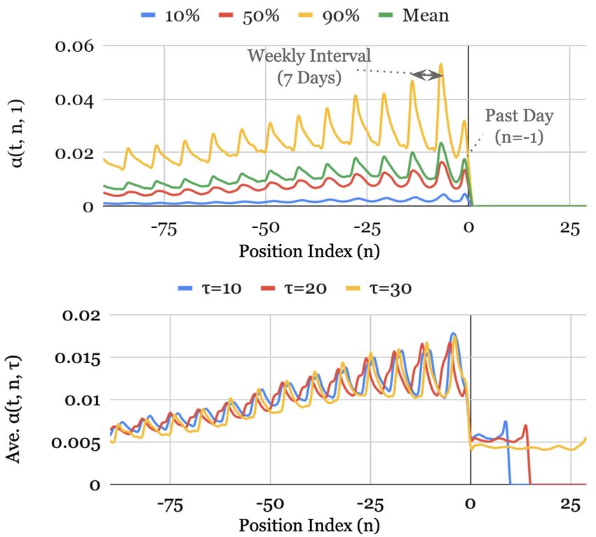
Iterated approaches utilize one-step-ahead prediction models, with multi-
step predictions obtained by recursively feeding predictions into future inputs.
Approaches with Long Short-term Memory (LSTM) [20] networks have been
considered, such as Deep AR [9] which uses stacked LSTM layers to generate pa-
rameters of one-step-ahead Gaussian predictive distributions. Deep State-Space
Models (DSSM) [6] adopt a similar approach, utilizing LSTMs to generate pa-
rameters of a predefined linear state-space model with predictive distributions
produced via Kalman filtering – with extensions for multivariate time series data
in [21]. More recently, Transformer-based architectures have been explored in
[12], which proposes the use of convolutional layers for local processing and a
sparse attention mechanism to increase the size of the receptive field during
forecasting. Despite their simplicity, iterative methods rely on the assumption
that the values of all variables excluding the target are known at forecast time
– such that only the target needs to be recursively fed into future inputs. How-
ever, in many practical scenarios, numerous useful time-varying inputs exist,
with many unknown in advance. Their straightforward use is hence limited for
iterative approaches. TFT, on the other hand, explicitly accounts for the di-
versity of inputs – naturally handling static covariates and (past-observed and
future-known) time-varying inputs.
    In contrast, direct methods are trained to explicitly generate forecasts for
multiple predefined horizons at each time step. Their architectures typically rely
on sequence-to-sequence models, e.g. LSTM encoders to summarize past inputs,
and a variety of methods to generate future predictions. The Multi-horizon
Quantile Recurrent Forecaster (MQRNN) [10] uses LSTM or convolutional en-
coders to generate context vectors which are fed into multi-layer perceptrons
(MLPs) for each horizon. In [11] a multi-modal attention mechanism is used
with LSTM encoders to construct context vectors for a bi-directional LSTM
decoder. Despite performing better than LSTM-based iterative methods, inter-
pretability remains challenging for such standard direct methods. In contrast,
we show that by interpreting attention patterns, TFT can provide insightful
explanations about temporal dynamics, and do so while maintaining state-of-
the-art performance on a variety of datasets.
    Time Series Interpretability with Attention: Attention mechanisms
are used in translation [17], image classification [22] or tabular learning [23]
to identify salient portions of input for each instance using the magnitude of
attention weights. Recently, they have been adapted for time series with inter-
pretability motivations [7, 12, 24], using LSTM-based [25] and transformer-based
[12] architectures. However, this was done without considering the importance
of static covariates (as the above methods blend variables at each input). TFT
alleviates this by using separate encoder-decoder attention for static features
at each time step on top of the self-attention to determine the contribution
time-varying inputs.
    Instance-wise Variable Importance with DNNs: Instance (i.e. sample)-
wise variable importance can be obtained with post-hoc explanation methods
[15, 16, 26] and inherently intepretable models [27, 24]. Post-hoc explanation
methods, e.g. LIME [15], SHAP [16] and RL-LIM [26], are applied on pre-

                                       4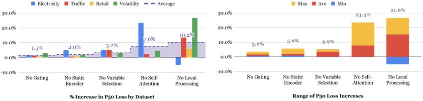
trained black-box models and often based on distilling into a surrogate inter-
pretable model, or decomposing into feature attributions. They are not de-
signed to take into account the time ordering of inputs, limiting their use for
complex time series data. Inherently-interpretable modeling approaches build
components for feature selection directly into the architecture. For time series
forecasting specifically, they are based on explicitly quantifying time-dependent
variable contributions. For example, Interpretable Multi-Variable LSTMs [27]
partitions the hidden state such that each variable contributes uniquely to its
own memory segment, and weights memory segments to determine variable
contributions. Methods combining temporal importance and variable selection
have also been considered in [24], which computes a single contribution coeffi-
cient based on attention weights from each. However, in addition to the short-
coming of modelling only one-step-ahead forecasts, existing methods also focus
on instance-specific (i.e. sample-specific) interpretations of attention weights
– without providing insights into global temporal dynamics. In contrast, the
use cases in Sec. 7 demonstrate that TFT is able to analyze global temporal
relationships and allows users to interpret global behaviors of the model on the
whole dataset – specifically in the identification of any persistent patterns (e.g.
seasonality or lag effects) and regimes present.

3. Multi-horizon Forecasting

    Let there be I unique entities in a given time series dataset – such as different
stores in retail or patients in healthcare. Each entity i is associated with a
set of static covariates si ∈ Rms , as well as inputs χi,t ∈ Rmχ and scalar
targets yi,t ∈ R at each time-step t ∈ [0, Ti ]. Time-dependent input features are
                                               T T T
subdivided into two categories χi,t = zi,t           , xi,t – observed inputs zi,t ∈ R(mz )
which can only be measured at each step and are unknown beforehand, and
known inputs xi,t ∈ Rmx which can be predetermined (e.g. the day-of-week at
time t).
    In many scenarios, the provision for prediction intervals can be useful for
optimizing decisions and risk management by yielding an indication of likely
best and worst-case values that the target can take. As such, we adopt quantile
regression to our multi-horizon forecasting setting (e.g. outputting the 10th ,
50th and 90th percentiles at each time step). Each quantile forecast takes the
form:
                 ŷi (q, t, τ ) = fq (τ, yi,t−k:t , zi,t−k:t , xi,t−k:t+τ , si ) ,     (1)
where ŷi,t+τ (q, t, τ ) is the predicted q th sample quantile of the τ -step-ahead
forecast at time t, and fq (.) is a prediction model. In line with other direct
methods, we simultaneously output forecasts for τmax time steps – i.e. τ ∈
{1, . . . , τmax }. We incorporate all past information within a finite look-back
window k, using target and known inputs only up till and including the forecast
start time t (i.e. yi,t−k:t = {yi,t−k , . . . , yi,t }) and known inputs across the entire

                                            5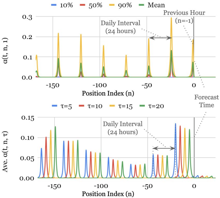
                                            2
range (i.e. xi,t−k:t+τ = xi,t−k , . . . , xi,t , . . . , xi,t+τ ).

4. Model Architecture

Figure 2: TFT architecture. TFT inputs static metadata, time-varying past inputs and time-
varying a priori known future inputs. Variable Selection is used for judicious selection of
the most salient features based on the input. Gated Residual Network blocks enable efficient
information flow with skip connections and gating layers. Time-dependent processing is based
on LSTMs for local processing, and multi-head attention for integrating information from any
time step.

    We design TFT to use canonical components to efficiently build feature
representations for each input type (i.e. static, known, observed inputs) for high
forecasting performance on a wide range of problems. The major constituents
of TFT are:
1. Gating mechanisms to skip over any unused components of the architec-
   ture, providing adaptive depth and network complexity to accommodate a
   wide range of datasets and scenarios.
2. Variable selection networks to select relevant input variables at each time
   step.
3. Static covariate encoders to integrate static features into the network,
   through encoding of context vectors to condition temporal dynamics.
4. Temporal processing to learn both long- and short-term temporal rela-
   tionships from both observed and known time-varying inputs. A sequence-
   to-sequence layer is employed for local processing, whereas long-term depen-
   dencies are captured using a novel interpretable multi-head attention block.

   2 For   notation simplicity, we omit the subscript i unless explicitly required.

                                                 6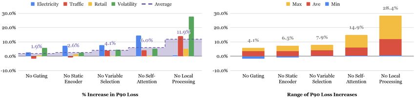
5. Prediction intervals via quantile forecasts to determine the range of likely
   target values at each prediction horizon.
    Fig. 2 shows the high level architecture of Temporal Fusion Transformer
(TFT), with individual components described in detail in the subsequent sec-
tions.

4.1. Gating Mechanisms
    The precise relationship between exogenous inputs and targets is often un-
known in advance, making it difficult to anticipate which variables are relevant.
Moreover, it is difficult to determine the extent of required non-linear process-
ing, and there may be instances where simpler models can be beneficial – e.g.
when datasets are small or noisy. With the motivation of giving the model the
flexibility to apply non-linear processing only where needed, we propose Gated
Residual Network (GRN) as shown in in Fig. 2 as a building block of TFT. The
GRN takes in a primary input a and an optional context vector c and yields:

          GRNω (a, c) = LayerNorm (a + GLUω (η1 )) ,                          (2)
                     η1 = W1,ω η2 + b1,ω ,                                    (3)
                     η2 = ELU (W2,ω a + W3,ω c + b2,ω ) ,                     (4)

where ELU is the Exponential Linear Unit activation function [28], η1 ∈ Rdmodel , η2 ∈
Rdmodel are intermediate layers, LayerNorm is standard layer normalization of
[29], and ω is an index to denote weight sharing. When W2,ω a + W3,ω c +
b2,ω >> 0, the ELU activation would act as an identity function and when
W2,ω a + W3,ω c + b2,ω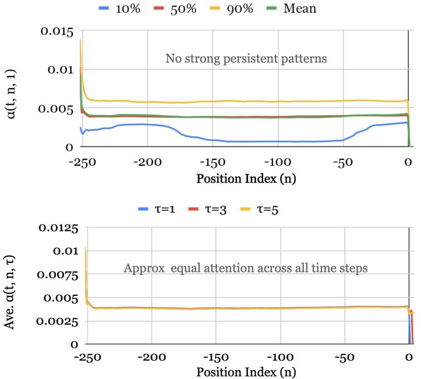
instance-wise variable selection through the use of variable selection networks
applied to both static covariates and time-dependent covariates. Beyond provid-
ing insights into which variables are most significant for the prediction problem,
variable selection also allows TFT to remove any unnecessary noisy inputs which
could negatively impact performance. Most real-world time series datasets con-
tain features with less predictive content, thus variable selection can greatly
help model performance via utilization of learning capacity only on the most
salient ones.
    We use entity embeddings [31] for categorical variables as feature represen-
tations, and linear transformations for continuous variables – transforming each
input variable into a (dmodel )-dimensional vector which matches the dimensions
in subsequent layers for skip connections. All static, past and future inputs
make use of separate variable selection networks (as denoted by different colors
in Fig. 2). Without loss of generality, we present the variable selection network
for past inputs – noting that those for other inputs take the same form.
         (j)
    Let ξt ∈ Rdmodel denote the transformed input of the j-th variable at time
                                  iT
                 (1)T       (m )T
               h
t, with Ξt = ξt , . . . , ξt χ       being the flattened vector of all past inputs
at time t. Variable selection weights are generated by feeding both Ξt and an
external context vector cs through a GRN, followed by a Softmax layer:

                         vχt = Softmax GRNvχ (Ξt , cs ) ,                       (6)

where vχt ∈ Rmχ is a vector of variable selection weights, and cs is obtained
from a static covariate encoder (see Sec. 4.3). For static variables, we note
that the context vector cs is omitted – given that it already has access to static
information.
    At each time step, an additional layer of non-linear processing is employed
                 (j)
by feeding each ξt through its own GRN:

                               (j)             (j)
                             ξ̃t = GRNξ̃(j) ξt       ,                         (7)

        (j)
where ξ̃t is the processed feature vector for variable j. We note that each vari-
able has its own GRNξ(j) , with weights shared across all time steps t. Processed
features are then weighted by their variable selection weights and combined:
                                    Xm χ          (j)
                              ξ̃t =       vχ(j)
                                             t
                                                ξ̃t ,                         (8)
                                       j=1

        (j)
where vχt is the j-th element of vector vχt .

4.3. Static Covariate Encoders
    In contrast with other time series forecasting architectures, the TFT is care-
fully designed to integrate information from static metadata, using separate
GRN encoders to produce four different context vectors, cs , ce , cc , and ch .
These contect vectors are wired into various locations in the temporal fusion

                                        8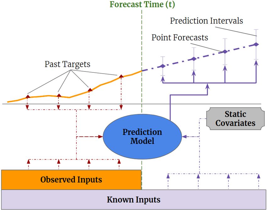
decoder (Sec. 4.5) where static variables play an important role in processing.
Specifically, this includes contexts for (1) temporal variable selection (cs ), (2)
local processing of temporal features (cc , ch ), and (3) enriching of temporal fea-
tures with static information (ce ). As an example, taking ζ to be the output
of the static variable selection network, contexts for temporal variable selection
would be encoded according to cs = GRNcs (ζ).

4.4. Interpretable Multi-Head Attention
    The TFT employs a self-attention mechanism to learn long-term relation-
ships across different time steps, which we modify from multi-head attention in
transformer-based architectures [17, 12] to enhance explainability. In general,
attention mechanisms scale values V ∈ RN ×dV based on relationships between
keys K ∈ RN ×dattn and queries Q ∈ RN ×dattn as below:

                       Attention(Q, K, V ) = A(Q, K)V ,                         (9)

where A() is a normalization function. A common choice is scaled dot-product
attention [17]:
                                              p
                    A(Q, K) = Softmax(QK T / dattn ).                   (10)

   To improve the learning capacity of the standard attention mechanism,
multi-head attention is proposed in [17], employing different heads for differ-
ent representation subspaces:

                  MultiHead(Q, K, V ) = [H1 , . . . , HmH ] WH ,               (11)
                                          (h)        (h)      (h)
                  Hh = Attention(Q       WQ , K     WK , V   WV ),             (12)
          (h)                      (h)                        (h)
where WK ∈ Rdmodel ×dattn , WQ ∈ Rdmodel ×dattn , WV ∈ Rdmodel ×dV are
head-specific weights for keys, queries and values, and WH ∈ R(mH ·dV )×dmodel
linearly combines outputs concatenated from all heads Hh .
    Given that different values are used in each head, attention weights alone
would not be indicative of a particular feature’s importance. As such, we modify
multi-head attention to share values in each head, and employ additive aggre-
gation of all heads:

            InterpretableMultiHead(Q, K, V ) = H̃ WH ,                         (13)

      H̃ = Ã(Q, K) V WV ,                                                     (14)
                XmH
                            (h)    (h)
         = 1/H        A Q W Q , K WK      V WV ,                               (15)
                       h=1
                  XmH                         (h)     (h)
          = 1/H            Attention(Q WQ , K WK , V WV ),                     (16)
                     h=1

where WV ∈ Rdmodel ×dV are value weights shared across all heads, and WH ∈
Rdattn ×dmodel is used for final linear mapping. From Eq. (15), we see that each

                                          9
head can learn different temporal patterns, while attending to a common set of
input features – which can be interpreted as a simple ensemble over attention
weights into combined matrix Ã(Q, K) in Eq. (14). Compared to A(Q, K) in
Eq. (10), Ã(Q, K) yields an increased representation capacity in an efficient
way.
4.5. Temporal Fusion Decoder
The temporal fusion decoder uses the series of layers described below to
learn temporal relationships present in the dataset:
4.5.1. Locality Enhancement with Sequence-to-Sequence Layer
In time series data, points of significance are often identified in relation
to their surrounding values – such as anomalies, change-points or cyclical pat-
terns. Leveraging local context, through the construction of features that utilize
pattern information on top of point-wise values, can thus lead to performance
improvements in attention-based architectures. For instance, [12] adopts a sin-
gle convolutional layer for locality enhancement – extracting local patterns us-
ing the same filter across all time. However, this might not be suitable for
cases when observed inputs exist, due to the differing number of past and fu-
ture inputs. As such, we propose the application of a sequence-to-sequence
model to naturally handle these differences – feeding ξ̃t−k:t into the encoder
and ξ̃t+1:t+τmax into the decoder. This then generates a set of uniform temporal
features which serve as inputs into the temporal fusion decoder itself – denoted
by φ(t, n) ∈ {φ(t, −k), . . . , φ(t, τmax )} with n being a position index. For com-
parability with commonly-used sequence-to-sequence baselines, we consider the
use of an LSTM encoder-decoder – although other models can potentially be
adopted as well. This also serves as a replacement for standard positional en-
coding, providing an appropriate inductive bias for the time ordering of the
inputs. Moreover, to allow static metadata to influence local processing, we use
the cc , ch context vectors from the static covariate encoders to initialize the cell
state and hidden state respectively for the first LSTM in the layer. We also
employ a gated skip connection over this layer:
φ̃(t, n) = LayerNorm ξ̃t+n + GLUφ̃ (φ(t, n)) , (17)
where n ∈ [−k, τmax ] is a position index.
4.5.2. Static Enrichment Layer
As static covariates often have a significant influence on the temporal dynam-
ics (e.g. genetic information on disease risk), we introduce a static enrichment
layer that enhances temporal features with static metadata. For a given position
index n, static enrichment takes the form:
θ(t, n) = GRNθ φ̃(t, n), ce , (18)
where the weights of GRNφ are shared across the entire layer, and ce is a context
vector from a static covariate encoder.
104.5.3. Temporal Self-Attention Layer
Following static enrichment, we next apply self-attention. All static-enriched
temporal features are first grouped into a single matrix – i.e. Θ(t) = [θ(t, −k), . . . ,
θ(t, τ )]T – and interpretable multi-head attention (see Sec. 4.4) is applied at
each forecast time (with N = τmax + k + 1):
B(t) = InterpretableMultiHead(Θ(t), Θ(t), Θ(t)), (19)
to yield B(t) = [β(t, −k), . . . , β(t, τmax )]. dV = dattn = dmodel /mH are cho-
sen, where mH is the number of heads. Decoder masking [17, 12] is applied to
the multi-head attention layer to ensure that each temporal dimension can only
attend to features preceding it. Besides preserving causal information flow via
masking, the self-attention layer allows TFT to pick up long-range dependen-
cies that may be challenging for RNN-based architectures to learn. Following
the self-attention layer, an additional gating layer is also applied to facilitate
training:
δ(t, n) = LayerNorm(θ(t, n) + GLUδ (β(t, n))). (20)
4.5.4. Position-wise Feed-forward Layer
We apply an additional non-linear processing to the outputs of the self-
attention layer. Similar to the static enrichment layer, this makes use of GRNs:
ψ(t, n) = GRNψ (δ(t, n)) , (21)
where the weights of GRNψ are shared across the entire layer. As per Fig. 2, we
also apply a gated residual connection which skips over the entire transformer
block, providing a direct path to the sequence-to-sequence layer – yielding a
simpler model if additional complexity is not required, as shown below:
ψ̃(t, n) = LayerNorm φ̃(t, n) + GLUψ̃ (ψ(t, n)) , (22)
4.6. Quantile Outputs
In line with previous work [10], TFT also generates prediction intervals on
top of point forecasts. This is achieved by the simultaneous prediction of various
percentiles (e.g. 10th , 50th and 90th ) at each time step. Quantile forecasts are
generated using linear transformation of the output from the temporal fusion
decoder:
ŷ(q, t, τ ) = Wq ψ̃(t, τ ) + bq , (23)
where Wq ∈ R1×d , bq ∈ R are linear coefficients for the specified quantile q.
We note that forecasts are only generated for horizons in the future – i.e. τ ∈
{1, . . . , τmax }.
115. Loss Functions
TFT is trained by jointly minimizing the quantile loss [10], summed across
all quantile outputs:
X X Xτmax QL (yt , ŷ(q, t − τ, τ ), q)
L(Ω, W ) = (24)
yt ∈Ω q∈Q τ =1 M τmax
QL(y, ŷ, q) = q(y − ŷ)+ + (1 − q)(ŷ − y)+ , (25)
where Ω is the domain of training data containing M samples, W represents the
weights of TFT, Q is the set of output quantiles (we use Q = {0.1, 0.5, 0.9} in
our experiments, and (.)+ = max(0, .). For out-of-sample testing, we evaluate
the normalized quantile losses across the entire forecasting horizon – focusing
on P50 and P90 risk for consistency with previous work [9, 6, 12]:
P Pτ
2 yt ∈Ω̃ τmax=1 QL (yt , ŷ(q, t − τ, τ ), q)
q-Risk = P Pτmax , (26)
yt ∈Ω̃ τ =1 |yt |
where Ω̃ is the domain of test samples. Full details on hyperparameter opti-
mization and training can be found in Appendix A.
6. Performance Evaluation
6.1. Datasets
We choose datasets to reflect commonly observed characteristics across a
wide range of challenging multi-horizon forecasting problems. To establish a
baseline and position with respect to prior academic work, we first evaluate
performance on the Electricity and Traffic datasets used in [9, 6, 12] – which
focus on simpler univariate time series containing known inputs only alongside
the target. Next, the Retail dataset helps us benchmark the model using the
full range of complex inputs observed in multi-horizon prediction applications
(see Sec. 3) – including rich static metadata and observed time-varying inputs.
Finally, to evaluate robustness to over-fitting on smaller noisy datasets, we
consider the financial application of volatility forecasting – using a dataset much
smaller than others. Broad descriptions of each dataset can be found below:
• Electricity: The UCI Electricity Load Diagrams Dataset, containing the
electricity consumption of 370 customers – aggregated on an hourly level as
in [32]. In accordance with [9], we use the past week (i.e. 168 hours) to
forecast over the next 24 hours.
• Traffic: The UCI PEM-SF Traffic Dataset describes the occupancy rate (with
yt ∈ [0, 1]) of 440 SF Bay Area freeways – as in [32]. It is also aggregated on
an hourly level as per the electricity dataset, with the same look back window
and forecast horizon.
12• Retail: Favorita Grocery Sales Dataset from the Kaggle competition [33],
that combines metadata for different products and the stores, along with
other exogenous time-varying inputs sampled at the daily level. We forecast
log product sales 30 days into the future, using 90 days of past information.
• Volatility (or Vol.): The OMI realized library [34] contains daily realized
volatility values of 31 stock indices computed from intraday data, along with
their daily returns. For our experiments, we consider forecasts over the next
week (i.e. 5 business days) using information over the past year (i.e. 252
business days).
6.2. Training Procedure
For each dataset, we partition all time series into 3 parts – a training set
for learning, a validation set for hyperparameter tuning, and a hold-out test
set for performance evaluation. Hyperparameter optimization is conducted via
random search, using 240 iterations for Volatility, and 60 iterations for others.
Full search ranges for all hyperparameters are below, with datasets and optimal
model parameters listed in Table 1.
• State size – 10, 20, 40, 80, 160, 240, 320
• Dropout rate – 0.1, 0.2, 0.3, 0.4, 0.5, 0.7, 0.9
• Minibatch size – 64, 128, 256
• Learning rate – 0.0001, 0.001, 0.01
• Max. gradient norm – 0.01, 1.0, 100.0
• Num. heads – 1, 4
To preserve explainability, we adopt only a single interpretable multi-head
attention layer. For ConvTrans [12], we use the same fixed stack size (3 layers)
and number of heads (8 heads) as in [12]. We keep the same attention model,
and treat kernel sizes for the convolutional processing layer as a hyperparameter
(∈ {1, 3, 6, 9}) – as optimal kernel sizes are observed to be dataset dependent
[12]. An open-source implementation of the TFT on these datasets can be found
on GitHub3 for full reproducibility.
6.3. Computational Cost
Across all datasets, each TFT model was also trained on a single GPU, and
can be deployed without the need for extensive computing resources. For in-
stance, using a NVIDIA Tesla V100 GPU, our optimal TFT model (for Electric-
ity dataset) takes just slightly over 6 hours to train (each epoch being roughly
52 mins). The batched inference on the entire validation dataset (consisting
50,000 samples) takes 8 minutes. TFT training and inference times can be
further reduced with hardware-specific optimizations.
13Table 1: Information on dataset and optimal TFT configuration.
Electricity Traffic Retail Vol.
Dataset Details
Target Type R [0, 1] R R
Number of Entities 370 440 130k 41
Number of Samples 500k 500k 500k ∼100k
Network Parameters
k 168 168 90 252
τmax 24 24 30 5
Dropout Rate 0.1 0.3 0.1 0.3
State Size 160 320 240 160
Number of Heads 4 4 4 1
Training Parameters
Minibatch Size 64 128 128 64
Learning Rate 0.001 0.001 0.001 0.01
Max Gradient Norm 0.01 100 100 0.01
6.4. Benchmarks
We extensively compare TFT to a wide range of models for multi-horizon
forecasting, based on the categories described in Sec. 2. Hyperparameter op-
timization is conducted using random search over a pre-defined search space,
using the same number of iterations across all benchmarks for a give dataset.
Additional details are included in Appendix A.
Direct methods: As TFT falls within this class of multi-horizon models,
we primarily focus comparisons on deep learning models which directly generate
prediction at future horizons, including: 1) simple sequence-to-sequence models
with global contexts (Seq2Seq), and 2) the Multi-horizon Quantile Recurrent
Forecaster (MQRNN) [10].
Iterative methods: To position with respect to the rich body of work on
iterative models, we evaluate TFT using the same setup as [9] for the Electricity
and Traffic datasets. This extends the results from [12] for 1) DeepAR [9], 2)
DSSM [6], and 3) the Transformer-based architecture of [12] with local convo-
lutional processing – which refer to as ConvTrans. For more complex datasets,
we focus on the ConvTrans model given its strong outperformance over other
iterative models in prior work, and DeepAR due to its popularity among practi-
tioners. As models in this category require knowledge of all inputs in the future
to generate predictions, we accommodate this for complex datasets by imputing
unknown inputs with their last available value.
For simpler univariate datasets, we note that the results for ARIMA, ETS,
TRMF, DeepAR, DSSM and ConvTrans have been reproduced from [12] in
3 URL: https://github.com/google-research/google-research/tree/master/tft
14Table 2: P50 and P90 quantile losses on a range of real-world datasets. Percentages in brackets
reflect the increase in quantile loss versus TFT (lower q-Risk better), with TFT outperforming
competing methods across all experiments, improving on the next best alternative method
(underlined) between 3% and 26%.
ARIMA ETS TRMF DeepAR DSSM
Electricity 0.154 (+180% ) 0.102 (+85% ) 0.084 (+53% ) 0.075 (+36% ) 0.083 (+51% )
Traffic 0.223 (+135% ) 0.236 (+148% ) 0.186 (+96% ) 0.161 (+69% ) 0.167 (+76% )
ConvTrans Seq2Seq MQRNN TFT
Electricity 0.059 (+7% ) 0.067 (+22% ) 0.077 (+40% ) 0.055*
Traffic 0.122 (+28% ) 0.105 (+11% ) 0.117 (+23% ) 0.095*
(a) P50 losses on simpler univariate datasets.
ARIMA ETS TRMF DeepAR DSSM
Electricity 0.102 (+278% ) 0.077 (+185% ) - 0.040 (+48% ) 0.056 (+107% )
Traffic 0.137 (+94% ) 0.148 (+110% ) - 0.099 (+40% ) 0.113 (+60% )
ConvTrans Seq2Seq MQRNN TFT
Electricity 0.034 (+26% ) 0.036 (+33% ) 0.036 (+33% ) 0.027*
Traffic 0.081 (+15% ) 0.075 (+6% ) 0.082 (+16% ) 0.070*
(b) P90 losses on simpler univariate datasets.
DeepAR CovTrans Seq2Seq MQRNN TFT
Vol. 0.050 (+28% ) 0.047 (+20% ) 0.042 (+7% ) 0.042 (+7% ) 0.039*
Retail 0.574 (+62% ) 0.429 (+21% ) 0.411 (+16% ) 0.379 (+7% ) 0.354*
(c) P50 losses on datasets with rich static or observed inputs.
DeepAR CovTrans Seq2Seq MQRNN TFT
Vol. 0.024 (+21% ) 0.024 (+22% ) 0.021 (+8% ) 0.021 (+9% ) 0.020*
Retail 0.230 (+56% ) 0.192 (+30% ) 0.157 (+7% ) 0.152 (+3% ) 0.147*
(d) P90 losses on datasets with rich static or observed inputs.
15Table 2 for consistency.
6.5. Results and Discussion
Table 2 shows that TFT significantly outperforms all benchmarks over the
variety of datasets described in Sec. 6.1. For median forecasts, TFT yields
7% lower P50 and 9% lower P90 losses on average compared to the next best
model – demonstrating the benefits of explicitly aligning the architecture with
the general multi-horizon forecasting problem.
Comparing direct and iterative models, we observe the importance of ac-
counting for the observed inputs – noting the poorer results of ConvTrans on
complex datasets where observed input imputation is required (i.e. Volatility
and Retail). Furthermore, the benefits of quantile regression are also observed
when targets are not captured well by Gaussian distributions with direct models
outperforming in those scenarios. This can be seen, for example, from the Traf-
fic dataset where target distribution is significantly skewed – with more than
90% of occupancy rates falling between 0 and 0.1, and the remainder distributed
evenly until 1.0.
6.6. Ablation Analysis
To quantify the benefits of each of our proposed architectural contribution,
we perform an extensive ablation analysis – removing each component from the
network as below, and quantifying the percentage increase in loss versus the
original architecture:
• Gating layers: We ablate by replacing each GLU layer (Eq. (5)) with a
simple linear layer followed by ELU.
• Static covariate encoders: We ablate by setting all context vectors to zero
– i.e. cs =ce =cc =ch =0 – and concatenating all transformed static inputs to
all time-dependent past and future inputs.
• Instance-wise variable selection networks: We ablate by replacing the
softmax outputs of Eq. 6 with trainable coefficients, and removing the net-
works generating the variable selection weights. We retain, however, the
variable-wise GRNs (see Eq. (7)), maintaining a similar amount of non-linear
processing.
• Self-attention layers: We ablate by replacing the attention matrix of the
interpretable multi-head attention layer (Eq. 14) with a matrix of trainable
parameters WA – i.e. Ã(Q, K) = WA , where WA ∈ RN ×N . This prevents
TFT from attending to different input features at different times, helping
evaluation of the importance of instance-wise attention weights.
• Sequence-to-sequence layers for local processing: We ablate by re-
placing the sequence-to-sequence layer of Sec. 4.5.1 with standard positional
encoding used in [17].
Ablated networks are trained across for each dataset using the hyperparam-
eters of Table 1. Fig. 3 shows that the effects on both P50 and P90 losses
are similar across all datasets, with all components contributing to performance
improvements on the whole.
16In general, the components responsible for capturing temporal relationships,
local processing and self-attention layers, have the largest impact on perfor-
mance, with P90 loss increases of > 6% on average and > 20% on select datasets
when ablated. The diversity across time series datasets can also be seen from the
differences in the ablation impact of the respective temporal components. Con-
cretely, while local processing is critical in Traffic, Retail and Volatility, lower
post-ablation P50 losses indicate that it can be detrimental in Electricity – with
the self-attention layer playing a more vital role. A possible explanation is that
persistent daily seasonality appears to dominate other temporal relationships in
the Electricity dataset. For this dataset, Table B.4 of Appendix B also shows
that the hour-of-day has the largest variable importance score across all tem-
poral inputs, exceeding even the target (i.e. Power Usage) itself. In contrast to
other dataset where past target observations are more significant (e.g. Traffic),
direct attention to previous days seem to help learning daily seasonal patterns
in Electricity – with local processing between adjacent time steps being less
necessary. We can account for this by treating the sequence-to-sequence archi-
tecture in the temporal fusion decoder as a hyperparameter to tune, including
an option for simple positional encoding without any local processing.
Static covariate encoders and instance-wise variable selection have the next
largest impact – increasing P90 losses by more than 2.6% and 4.1% on average.
The biggest benefits of these are observed for electricity dataset, where some of
the input features get very low importance.
Finally, gating layer ablation also shows increases in P90 losses, with a 1.9%
increase on average. This is the most significant on the volatility (with a 4.1%
P90 loss increase), underlying the benefit of component gating for smaller and
noisier datasets.
7. Interpretability Use Cases
Having established the performance benefits of our model, we next demon-
strate how our model design allows for analysis of its individual components
to interpret the general relationships it has learned. We demonstrate three in-
terpretability use cases: (1) examining the importance of each input variable
in prediction, (2) visualizing persistent temporal patterns, and (3) identifying
any regimes or events that lead to significant changes in temporal dynamics. In
contrast to other examples of attention-based interpretability [25, 12, 7] which
zoom in on interesting but instance-specific examples, our methods focus on
ways to aggregate the patterns across the entire dataset – extracting generaliz-
able insights about temporal dynamics.
7.1. Analyzing Variable Importance
We first quantify variable importance by analyzing the variable selection
weights described in Sec. 4.2. Concretely, we aggregate selection weights (i.e.
(j)
vχt in Eq. (8)) for each variable across our entire test set, recording the 10th ,
50th and 90th percentiles of each sampling distribution. As the Retail dataset
17Table 3: Variable importance for the Retail dataset. The 10th , 50th and 90th percentiles of
the variable selection weights are shown, with values larger than 0.1 highlighted in purple.
For static covariates, the largest weights are attributed to variables which uniquely identify
different entities (i.e. item number and store number). For past inputs, past values of the
target (i.e. log sales) are critical as expected, as forecasts are extrapolations of past observa-
tions. For future inputs, promotion periods and national holidays have the greatest influence
on sales forecasts, in line with periods of increased customer spending.
10% 50% 90% 10% 50% 90%
Item Num 0.198 0.230 0.251 Transactions 0.029 0.033 0.037
Store Num 0.152 0.161 0.170 Oil 0.062 0.081 0.105
City 0.094 0.100 0.124 On-promotion 0.072 0.075 0.078
State 0.049 0.060 0.083 Day of Week 0.007 0.007 0.008
Type 0.005 0.006 0.008 Day of Month 0.083 0.089 0.096
Cluster 0.108 0.122 0.133 Month 0.109 0.122 0.136
Family 0.063 0.075 0.079 National Hol 0.131 0.138 0.145
Class 0.148 0.156 0.163 Regional Hol 0.011 0.014 0.018
Perishable 0.084 0.085 0.088 Local Hol 0.056 0.068 0.072
Open 0.027 0.044 0.067
Log Sales 0.304 0.324 0.353
(a) Static Covariates (b) Past Inputs
10% 50% 90%
On-promotion 0.155 0.170 0.182
Day of Week 0.029 0.065 0.089
Day of Month 0.056 0.116 0.138
Month 0.111 0.155 0.240
National Hol 0.145 0.220 0.242
Regional Hol 0.012 0.014 0.060
Local Hol 0.116 0.151 0.239
Open 0.088 0.095 0.097
(c) Future Inputs
18(a) Changes in P50 losses across ablation tests
(b) Changes in P90 losses across ablation tests
Figure 3: Results of ablation analysis. Both a) and b) show the impact of ablation on the
P50 and P90 losses respectively. Results per dataset shown on the left, and the range across
datasets shown on the right. While the precise importance of each is dataset-specific, all
components contribute significantly on the whole – with the maximum percentage increase
over all datasets ranging from 3.6% to 23.4% for P50 losses, and similarly from 4.1% to 28.4%
for P90 losses.
contains the full set of available input types (i.e. static metadata, known inputs,
observed inputs and the target), we present the results for its variable impor-
tance analysis in Table 3. We also note similar findings in other datasets, which
are documented in Appendix B.1 for completeness. On the whole, the results
show that the TFT extracts only a subset of key inputs that intuitively play a
significant role in predictions. The analysis of persistent temporal patterns is
often key to understanding the time-dependent relationships present in a given
dataset. For instance, lag models are frequently adopted to study length of time
required for an intervention to take effect [35] – such as the impact of a govern-
ment’s increase in public expenditure on the resultant growth in Gross National
Product [36]. Seasonality models are also commonly used in econometrics to
identify periodic patterns in a target-of-interest [37] and measure the length of
each cycle. From a practical standpoint, model builders can use these insights to
further improve the forecasting model – for instance by increasing the receptive
field to incorporate more history if attention peaks are observed at the start of
the lookback window, or by engineering features to directly incorporate seasonal
effects. As such, using the attention weights present in the self-attention layer of
the temporal fusion decoder, we present a method to identify similar persistent
patterns – by measuring the contributions of features at fixed lags in the past
on forecasts at various horizons. Combining Eq. (14) and (19), we see that the
self-attention layer contains a matrix of attention weights at each forecast time
t – i.e. Ã(φ(t), φ(t)). Multi-head attention outputs at each forecast horizon τ
19(i.e. β(t, τ )) can then be described as an attention-weighted sum of lower level
features at each position n:
Xτmax
β(t, τ ) = α(t, n, τ ) θ̃(t, n), (27)
n=−k
where α(t, n, τ ) is the (τ, n)-th element of Ã(φ(t), φ(t)), and θ̃(t, n) is a row
of Θ̃(t) = Θ(t)WV . Due to decoder masking, we also note that α(t, i, j) = 0,
∀i > j. For each forecast horizon τ , the importance of a previous time point
n < τ can hence be determined by analyzing distributions of α(t, n, τ ) across
all time steps and entities.
7.2. Visualizing Persistent Temporal Patterns
Attention weight patterns can be used to shed light on the most important
past time steps that the TFT model bases its decisions on. In contrast to other
traditional and machine learning time series methods, which rely on model-
based specifications for seasonality and lag analysis, the TFT can learn such
patterns from raw training data.
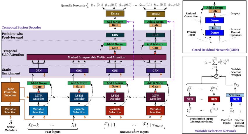
Fig. 4 shows the attention weight patterns across all our test datasets –
with the upper graph plotting the mean along with the 10th , 50th and 90th
percentiles of the attention weights for one-step-ahead forecasts (i.e. α(t, 1, τ ))
over the test set, and the bottom graph plotting the average attention weights
for various horizons (i.e. τ ∈ {5, 10, 15, 20}). We observe that the three datasets
exhibit a seasonal pattern, with clear attention spikes at daily intervals observed
for Electricity and Traffic, and a slightly weaker weekly patterns for Retail.
For Retail, we also observe the decaying trend pattern, with the last few days
dominating the importance.
No strong persistent patterns were observed for the Volatility – attention
weights equally distributed across all positions on average. This resembles a
moving average filter at the feature level, and – given the high degree of ran-
domness associated with the volatility process – could be useful in extracting
the trend over the entire period by smoothing out high-frequency noise.
TFT learns these persistent temporal patterns from the raw training data
without any human hard-coding. Such capability is expected to be very useful
in building trust with human experts via sanity-checking. Model developers can
also use these towards model improvements, e.g. via specific feature engineering
or data collection.
7.3. Identifying Regimes & Significant Events
Identifying sudden changes in temporal patterns can also be very useful,
as temporary shifts can occur due to the presence of significant regimes or
events. For instance, regime-switching behavior has been widely documented in
financial markets [38], with returns characteristics – such as volatility – being
observed to change abruptly between regimes. As such, identifying such regime
changes provides strong insights into the underlying problem which is useful for
identification of the significant events.
20(a) Electricity (b) Traffic
(c) Retail (d) Volatility
Figure 4: Persistent temporal patterns across datasets. Clear seasonality observed for the
Electricity, Traffic and Retail datasets, but no strong persistent patterns seen in Volatility
dataset. Upper plot – percentiles of attention weights for one-step-ahead forecast. Lower plot
– average attention weights for forecast at various horizons.
21Figure 5: Regime identification for S&P 500 realized volatility. Significant deviations in
attention patterns can be observed around periods of high volatility – corresponding to the
peaks observed in dist(t). We use a threshold of dist(t) > 0.3 to denote significant regimes, as
highlighted in purple. Focusing on periods around the 2008 financial crisis, the top right plot
visualizes α(t, n, 1) midway through the significant regime, compared to the normal regime on
the top left.
Firstly, for a given entity, we define the average attention pattern per forecast
horizon as: XT
ᾱ(n, τ ) = α(t, j, τ )/T, (28)
t=1
and then construct ᾱ(τ ) = [ᾱ(−k, τ ), . . . , ᾱ(τmax , τ )]T . To compare similarities
between attention weight vectors, we use the distance metric proposed by [39]:
p
κ(p, q) = 1 − ρ(p, q), (29)
P √
where ρ(p, q) = j pj qj is the Bhattacharya coefficient [40] measuring the
overlap between discrete distributions – with pj , qj being elements of probability
vectors p, q respectively. For each entity, significant shifts in temporal dynamics
are then measured using the distance between attention vectors at each point
with the average pattern, aggregated for all horizons as below:
Xτmax
dist(t) = κ ᾱ(τ ), α(t, τ ) /τmax , (30)
τ =1
where α(t, τ ) = [α(t, −k, τ ), . . . , α(t, τmax , τ )]T .
Using the volatility dataset, we attempt to analyse regimes by applying our
distance metric to the attention patterns for the S&P 500 index over our train-
ing period (2001 to 2015). Plotting dist(t) against the target (i.e. log realized
volatility) in the bottom chart of Fig. 5, significant deviations in attention pat-
terns can be observed around periods of high volatility (e.g. the 2008 financial
crisis) – corresponding to the peaks observed in dist(t). From the plots, we can
22see that TFT appears to alter its behaviour between regimes – placing equal at-
tention across past inputs when volatility is low, while attending more to sharp
trend changes during high volatility periods – suggesting differences in temporal
dynamics learned in each of these cases.
8. Conclusions
We introduce TFT, a novel attention-based deep learning model for in-
terpretable high-performance multi-horizon forecasting. To handle static co-
variates, a priori known inputs, and observed inputs effectively across wide
range of multi-horizon forecasting datasets, TFT uses specialized components.
Specifically, these include: (1) sequence-to-sequence and attention based tempo-
ral processing components that capture time-varying relationships at different
timescales, (2) static covariate encoders that allow the network to condition
temporal forecasts on static metadata, (3) gating components that enable skip-
ping over unnecessary parts of the network, (4) variable selection to pick rel-
evant input features at each time step, and (5) quantile predictions to obtain
output intervals across all prediction horizons. On a wide range of real-world
tasks – on both simple datasets that contain only known inputs and complex
datasets which encompass the full range of possible inputs – we show that TFT
achieves state-of-the-art forecasting performance. Lastly, we investigate the gen-
eral relationships learned by TFT through a series of interpretability use cases
– proposing novel methods to use TFT to (i) analyze important variables for a
given prediction problem, (ii) visualize persistent temporal relationships learned
(e.g. seasonality), and (iii) identify significant regimes changes.
9. Acknowledgements
The authors gratefully acknowledge discussions with Yaguang Li, Maggie
Wang, Jeffrey Gu, Minho Jin and Andrew Moore that contributed to the devel-
opment of this paper.
23References
[1] J.-H. Böse, et al., Probabilistic demand forecasting at scale, Proc. VLDB Endow. 10 (12)
(2017) 1694–1705.
[2] P. Courty, H. Li, Timing of seasonal sales, The Journal of Business 72 (4) (1999) 545–572.
[3] B. Lim, A. Alaa, M. van der Schaar, Forecasting treatment responses over time using
recurrent marginal structural networks, in: NeurIPS, 2018.
[4] J. Zhang, K. Nawata, Multi-step prediction for influenza outbreak by an adjusted long
short-term memory, Epidemiology and infection 146 (7) (2018).
[5] C. Capistran, C. Constandse, M. Ramos-Francia, Multi-horizon inflation forecasts using
disaggregated data, Economic Modelling 27 (3) (2010) 666 – 677.
[6] S. S. Rangapuram, et al., Deep state space models for time series forecasting, in: NIPS,
2018.
[7] A. Alaa, M. van der Schaar, Attentive state-space modeling of disease progression, in:
NIPS, 2019.
[8] S. Makridakis, E. Spiliotis, V. Assimakopoulos, The m4 competition: 100,000 time series
and 61 forecasting methods, International Journal of Forecasting 36 (1) (2020) 54 – 74.
[9] D. Salinas, V. Flunkert, J. Gasthaus, T. Januschowski, DeepAR: Probabilistic forecasting
with autoregressive recurrent networks, International Journal of Forecasting (2019).
[10] R. Wen, et al., A multi-horizon quantile recurrent forecaster, in: NIPS 2017 Time Series
Workshop, 2017.
[11] C. Fan, et al., Multi-horizon time series forecasting with temporal attention learning, in:
KDD, 2019.
[12] S. Li, et al., Enhancing the locality and breaking the memory bottleneck of transformer
on time series forecasting, in: NeurIPS, 2019.
[13] J. Koutnı́k, K. Greff, F. Gomez, J. Schmidhuber, A clockwork rnn, in: ICML, 2014.
[14] D. Neil, et al., Phased lstm: Accelerating recurrent network training for long or event-
based sequences, in: NIPS, 2016.
[15] M. Ribeiro, et al., ”why should i trust you?” explaining the predictions of any classifier,
in: KDD, 2016.
[16] S. Lundberg, S.-I. Lee, A unified approach to interpreting model predictions, in: NIPS,
2017.
[17] A. Vaswani, N. Shazeer, N. Parmar, J. Uszkoreit, L. Jones, A. N. Gomez, L. u. Kaiser,
I. Polosukhin, Attention is all you need, in: NIPS, 2017.
[18] S. B. Taieb, A. Sorjamaa, G. Bontempi, Multiple-output modeling for multi-step-ahead
time series forecasting, Neurocomputing 73 (10) (2010) 1950 – 1957.
[19] M. Marcellino, J. Stock, M. Watson, A comparison of direct and iterated multistep ar
methods for forecasting macroeconomic time series, Journal of Econometrics 135 (2006)
499–526.
[20] S. Hochreiter, J. Schmidhuber, Long short-term memory, Neural Computation 9 (8)
(1997) 1735–1780.
24[21] Y. Wang, et al., Deep factors for forecasting, in: ICML, 2019.
[22] F. Wang, M. Jiang, C. Qian, S. Yang, C. Li, H. Zhang, X. Wang, X. Tang, Residual
attention network for image classification, in: CVPR, 2017.
[23] S. O. Arik, T. Pfister, Tabnet: Attentive interpretable tabular learning (2019). arXiv:
1908.07442.
[24] E. Choi, et al., Retain: An interpretable predictive model for healthcare using reverse
time attention mechanism, in: NIPS, 2016.
[25] H. Song, et al., Attend and diagnose: Clinical time series analysis using attention models,
2018.
[26] J. Yoon, S. O. Arik, T. Pfister, Rl-lim: Reinforcement learning-based locally interpretable
modeling (2019). arXiv:1909.12367.
[27] T. Guo, T. Lin, N. Antulov-Fantulin, Exploring interpretable LSTM neural networks
over multi-variable data, in: ICML, 2019.
[28] D.-A. Clevert, T. Unterthiner, S. Hochreiter, Fast and accurate deep network learning
by exponential linear units (ELUs), in: ICLR, 2016.
[29] J. Lei Ba, J. R. Kiros, G. E. Hinton, Layer Normalization, arXiv:1607.06450 (Jul 2016).
arXiv:1607.06450.
[30] Y. Dauphin, A. Fan, M. Auli, D. Grangier, Language modeling with gated convolutional
networks, in: ICML, 2017.
[31] Y. Gal, Z. Ghahramani, A theoretically grounded application of dropout in recurrent
neural networks, in: NIPS, 2016.
[32] H.-F. Yu, N. Rao, I. S. Dhillon, Temporal regularized matrix factorization for high-
dimensional time series prediction, in: NIPS, 2016.
[33] C. Favorita, Corporacion favorita grocery sales forecasting competition (2018).
URL https://www.kaggle.com/c/favorita-grocery-sales-forecasting/
[34] G. Heber, A. Lunde, N. Shephard, K. K. Sheppard, Oxford-man institute’s realized
library (2009).
URL https://realized.oxford-man.ox.ac.uk/
[35] S. Du, G. Song, L. Han, H. Hong, Temporal causal inference with time lag, Neural
Computation 30 (1) (2018) 271–291.
[36] B. Baltagi, Distributed Lags and Dynamic Models, 2008, pp. 129–145.
[37] S. Hylleberg (Ed.), Modelling Seasonality, Oxford University Press, 1992.
[38] A. Ang, A. Timmermann, Regime changes and financial markets, Annual Review of
Financial Economics 4 (1) (2012) 313–337.
[39] D. Comaniciu, V. Ramesh, P. Meer, Kernel-based object tracking, IEEE Transactions on
Pattern Analysis and Machine Intelligence 25 (5) (2003) 564–577.
[40] T. Kailath, The divergence and bhattacharyya distance measures in signal selection,
IEEE Transactions on Communication Technology 15 (1) (1967) 52–60.
[41] E. Giovanis, The turn-of-the-month-effect: Evidence from periodic generalized autore-
gressive conditional heteroskedasticity (pgarch) model, International Journal of Economic
Sciences and Applied Research 7 (2014) 43–61.
25You can also read