Object-driven Text-to-Image Synthesis via Adversarial Training
←
→
Page content transcription
If your browser does not render page correctly, please read the page content below
Object-driven Text-to-Image Synthesis via Adversarial Training

                                                                     Wenbo Li†∗1,2 Pengchuan Zhang∗2 Lei Zhang3
                                                              Qiuyuan Huang2 Xiaodong He4 Siwei Lyu1 Jianfeng Gao2
                                                 1
                                                   University at Albany, SUNY 2 Microsoft Research AI 3 Microsoft 4 JD AI Research
                                             {wli20,slyu}@albany.edu, {penzhan,leizhang,qihua,jfgao}@microsoft.com, xiaodong.he@jd.com
arXiv:1902.10740v1 [cs.CV] 27 Feb 2019

                                                                         Abstract

                                         In this paper, we propose Object-driven Attentive Gen-
                                         erative Adversarial Newtorks (Obj-GANs) that allow
                                         object-centered text-to-image synthesis for complex scenes.
                                         Following the two-step (layout-image) generation process,
                                         a novel object-driven attentive image generator is pro-
                                         posed to synthesize salient objects by paying attention to
                                         the most relevant words in the text description and the
                                         pre-generated semantic layout. In addition, a new Fast
                                         R-CNN based object-wise discriminator is proposed to
                                         provide rich object-wise discrimination signals on whether
                                         the synthesized object matches the text description and the
                                         pre-generated layout. The proposed Obj-GAN significantly
                                         outperforms the previous state of the art in various metrics
                                         on the large-scale COCO benchmark, increasing the
                                         Inception score by 27% and decreasing the FID score by
                                         11%. A thorough comparison between the traditional grid                   Figure 1: Top: AttnGAN [29] and its grid attention visualization.
                                         attention and the new object-driven attention is provided                 Middle: our modified implementation of two-step (layout-image)
                                         through analyzing their mechanisms and visualizing their                  generation proposed in [9]. Bottom: our Obj-GAN and its object-
                                         attention layers, showing insights of how the proposed                    driven attention visualization. The middle and bottom generations
                                         model generates complex scenes in high quality.                           use the same generated semantic layout, and the only difference is
                                                                                                                   the object-driven attention.
                                         1. Introduction
                                                                                                                   refinement for fine-grained text-to-image generation.
                                             Synthesizing images from text descriptions (known as                      Although images with realistic texture have been syn-
                                         Text-to-Image synthesis) is an important machine learning                 thesized on simple datasets, such as birds [29, 16] and
                                         task, which requires handling ambiguous and incomplete                    flowers [33], most existing approaches do not specifically
                                         information in natural language descriptions and learning                 model objects and their relations in images and thus have
                                         across vision and language modalities. Approaches based                   difficulties in generating complex scenes such as those in
                                         on Generative Adversarial Networks (GANs) [5] have re-                    the COCO dataset [15]. For example, generating images
                                         cently achieved promising results on this task [23, 22, 32,               from a sentence “several people in their ski gear are in the
                                         33, 29, 16, 9, 12, 34]. Most GAN based methods synthe-                    snow” requires modeling of different objects (people, ski
                                         size the image conditioned only on a global sentence vec-                 gear) and their interactions (people on top of ski gear), as
                                         tor, which may miss important fine-grained information at                 well as filling the missing information (e.g., the rocks in the
                                         the word level, and prevents the generation of high-quality               background). In the top row of Fig. 1, the image gener-
                                         images. More recently, AttnGAN [29] is proposed which                     ated by AttnGAN does contain scattered texture of people
                                         introduces the attention mechanism [28, 30, 2, 27] into the               and snow, but the shape of people are distorted and the pic-
                                         GAN framework, thus allows attention-driven, multi-stage                  ture’s layout is semantically not meaningful. [9] remedies
                                         † Work was performed when was an intern with Microsoft Research AI.       this problem by first constructing a semantic layout from the
                                         * indicates equal contributions.                                          text and then synthesizing the image by a deconvolutional

                                                                                                               1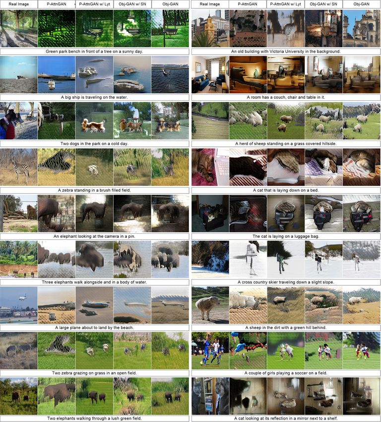
image generator. However, the fine-grained word/object-          through different approaches, such as variational infer-
level information is still not explicitly used for generation.   ence [17, 6], approximate Langevin process [24], condi-
Thus, the synthesized images do not contain enough details       tional PixelCNN via maximal likelihood estimation [26,
to make them look realistic (see the middle row of Fig. 1).      24], and conditional generative adversarial networks [23,
   In this study, we aim to generate high-quality complex        22, 32, 33]. Compared with other approaches, Generative
images with semantically meaningful layout and realistic         Adversarial Networks (GANs) [5] have shown better per-
objects. To this end, we propose a novel Object-driven At-       formance in image generation [21, 3, 25, 13, 11, 10]. How-
tentive Generative Adversarial Networks (Obj-GAN) that           ever, existing GAN based text-to-image synthesis is usu-
effectively capture and utilize fine-grained word/object-        ally conditioned only on the global sentence vector, which
level information for text-to-image synthesis. The Obj-          misses important fine-grained information at the word level,
GAN consists of a pair of object-driven attentive image          and thus lacks the ability to generate high-quality images.
generator and object-wise discriminator, and a new object-       [29] uses the traditional grid visual attention mechanism in
driven attention mechanism. The proposed image genera-           this task, which enables synthesizing fine-grained details at
tor takes as input the text description and a pre-generated      different image regions by paying attentions to the relevant
semantic layout and synthesize high-resolution images via        words in the text description.
multiple-stage coarse-to-fine process. At every stage, the          To explicitly encode the semantic layout into the gen-
generator synthesizes the image region within a bounding         erator, [9] proposes to decompose the generation process
box by focusing on words that are most relevant to the ob-       into two steps, in which it first constructs a semantic lay-
ject in that bounding box, as illustrated in the bottom row      out (bounding boxes and object shapes) from the text and
of Fig. 1. More specifically, using a new object-driven at-      then synthesizes an image conditioned on the layout and
tention layer, it uses the class label to query words in the     text description. [12] also proposes such a two-step process
sentences to form a word context vector, as illustrated in       to generate images from scene graphs, and their process can
Fig. 4, and then synthesizes the image region conditioned        be trained end-to-end. In this work, the proposed Obj-GAN
on the class label and word context vector. The object-wise      follows the two-step generation process as [9]. However,
discriminator checks every bounding box to make sure that        [9] encodes the text into a single global sentence vector,
the generated object indeed matches the pre-generated se-        which loses word-level fine-grained information. More-
mantic layout. To compute the discrimination losses for all      over, it uses the image-level GAN loss for the discriminator,
bounding boxes simultaneously and efficiently, our object-       which is less effective at providing object-wise discrimina-
wise discriminator is based on a Fast R-CNN [4], with a          tion signal for generating salient objects. We propose a new
binary cross-entropy loss for each bounding box.                 object-driven attention mechanism to provide fine-grained
   The contribution of this work is three-folded. (i) An         information (words in the text description and objects in
Object-driven Attentive Generative Network (Obj-GAN) is          the layout) for different components, including an attentive
proposed for synthesizing complex images from text de-           seq2seq bounding box generator, an attentive image gener-
scriptions. Specifically, two novel components are pro-          ator and an object-wise discriminator.
posed, including the object-driven attentive generative net-        The attention mechanism has recently become a crucial
work and the object-wise discriminator. (ii) Comprehen-          part of vision-language multi-modal intelligence tasks. The
sive evaluation on a large-scale COCO benchmark shows            traditional grid attention mechanism has been successfully
that our Obj-GAN significantly outperforms previous state-       used in modeling multi-level dependencies in image cap-
of-the-art text-to-image synthesis methods. Detailed abla-       tioning [28], image question answering [30], text-to-image
tion study is performed to empirically evaluate the effect of    generation [29], unconditional image synthesis [31] and
different components in Obj-GAN. (iii) A thorough analy-         image-to-image translation [16], image/text retrieval [14].
sis is performed through visualizing the attention layers of     In 2018, [1] proposes a bottom-up attention mechanism,
the Obj-GAN, showing insights of how the proposed model          which enables attention to be calculated over semantic
generates complex scenes in high quality. Compared with          meaningful regions/objects in the image, for image caption-
the previous work, our object-driven attention is more ro-       ing and visual question-answering. Inspired by these works,
bust and interpretable, and significantly improves the object    we propose Obj-GAN which for the first time develops an
generation quality in complex scenes.                            object-driven attentive generator plus an object-wise dis-
                                                                 criminator, thus enables GANs to synthesize high-quality
2. Related Work                                                  images of complicated scenes.
   Generating photo-realistic images from text descrip-          3. Object-driven Attentive GAN
tions, though challenging, is important to many real-world
applications such as art generation and computer-aided de-         As illustrated in Fig. 2, the Obj-GAN performs text-to-
sign. There has been much research effort for this task          image synthesis in two steps: generating a semantic layout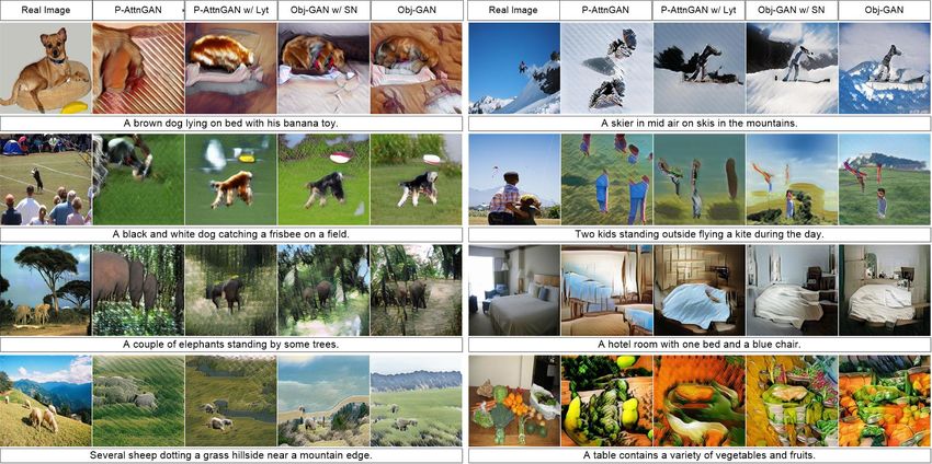
Figure 2: Obj-GAN completes the text-to-image synthesis in two steps: the layout generation and the image generation. The layout
generation contains a bounding box generator and a shape generator. The image generation uses the object-driven attentive image generator.
(class labels, bounding boxes, shapes of salient objects),              where zt ∼ N (0, 1) is a random noise vector. Since the
and then generating the image. In the image generation                  generated shapes not only need to match the location and
step, the object-driven attentive generator and object-wise             category information provided by B1:T , but also should be
discriminator are designed to enable image generation con-              aligned with its surrounding context, we build Gshape based
ditioned on the semantic layout generated in the first step.            on a bi-directional convolutional LSTM, as illustrated in
    The input of Obj-GAN is a sentence with Ts tokens.                  Fig. 2. Training of Gshape is based on the GAN framework
With a pre-trained bi-LSTM model, we encode its words                   [9], in which a perceptual loss is also used to constrain the
as word vectors e ∈ RD×Ts and the entire sentence as a                  generated shapes and to stabilize the training.
global sentence vector ē ∈ RD . We provide details of this
                                                                        3.2. Image generation
pre-trained bi-LSTM model and the implementation details
of other modules of Obj-GAN in § A.                                     3.2.1   Attentive multistage image generator
3.1. Semantic layout generation                                         As shown in Fig. 3, the proposed attentive multistage gen-
                                                                        erative network has two generators (G0 , G1 ). The base gen-
    In the first step, the Obj-GAN takes the sentence as input
                                                                        erator G0 first generates a low-resolution image x b0 condi-
and generates a semantic layout, a sequence of objects spec-
                                                                        tioned on the global sentence vector and the pre-generated
ified by their bounding boxes (with class labels) and shapes.
                                                                        semantic layout. The refiner G1 then refines details in dif-
As illustrated in Fig. 2, a box generator first generates a se-
                                                                        ferent regions by paying attention to most relevant words
quence of bounding boxes, and then a shape generator gen-
                                                                        and pre-generated class labels and generates a higher reso-
erates their shapes. This part resembles the bounding box
                                                                        lution image xb1 . Specifically,
generator and shape generator in [9], and we put our imple-
                                                                          h0 = F0 (z, ē, Enc(M 0 ), cobj , clab ), xb0 = G0 (h0 ),
mentation details in § A.
Box generator. We train an attentive seq2seq model [2],                   h1 = F1 (cpat , h0 + Enc(M 1 ), cobj , clab ), xb1 = G1 (h1 ),
also referring to Fig. 2, as the box generator:                         where (i) z is a random vector with standard normal distri-
                                                                        bution; (ii) Enc(M 0 ) ( Enc(M 1 ) ) is the encoding of low-
           B1:T := [B1 , B2 , . . . , BT ] ∼ Gbox (e).        (1)       resolution shapes M 0 (higher-resolution shapes M 1 ); (iii)
                                                                                  grid
Here, e are the pre-trained bi-LSTM word vectors, Bt =                  cpat = Fattn   (e, h0 ) are the patch-wise context vectors from
                                                                                                                         obj
(lt , bt ) are the class label of the t’s object and its bounding       the traditional grid attention, (iv) cobj = Fattn    (e, eg , lg , M )
box b = (x, y, w, h) ∈ R4 . In the rest of the paper, we will           are the object-wise context vectors from our new object-
also call the label-box pair Bt as a bounding box when no               driven attention, and clab = clab (lg , M ) are the label context
confusion arises. Since most of the bounding boxes have                 vectors from class labels. We can stack more refiners to the
corresponding words in the sentence, the attentive seq2seq              generation process and get higher and higher resolution im-
model captures this correspondence better than the seq2seq              ages. In this paper, we have two refiners (G1 and G2 ) and
model used in [9].                                                      finally generate images with resolution 256 × 256.
Shape generator. Given the bounding boxes B1:T , the                    Compute context vectors via attention. Both patch-wise
shape generator predicts the shape of each object in its                context vectors cpat and object-wise context vectors cobj are
bounding box, i.e.,                                                     attention-driven context vectors for specific image regions,
                                                                        and encode information from the words that are most rele-
                 M
                 c1:T = Gshape (B1:T , z1:T ).                (2)       vant to that image region. Patch-wise context vectors are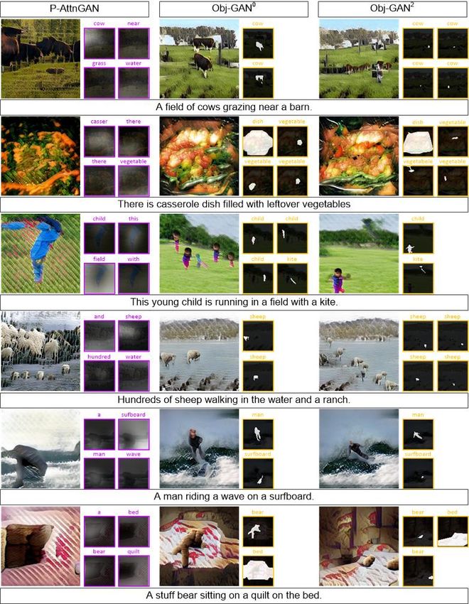
Figure 3: The object-driven attentive image generator.
                                                                         For the traditional grid attention, we use the image region
                                                                         feature hj , which is one column in the previous hidden layer
                                                                                      pat   pat
                                                                         h ∈ RD ×N , to query the pre-trained bi-LSTM word
                                                                         vectors e. For the new object-driven attention, we use the
                                                                         GloVe embedding of object class label ltg to query the GloVe
                                                                         embedding of the words in the sentence, as illustrated in the
                                                                         lower part of Fig. 4.
                                                                         Feature map concatenation. The patch-wise context vec-
                                                                         tor cpat
                                                                               j can be directly concatenated with the image feature
                                                                         vector hj in the previous layer. However, the object-wise
                                                                         context vector cobj   t cannot, because they are associated with
                  Figure 4: Object-driven attention.                     bounding      boxes    instead of pixels in the hidden feature map.
for uniform-partitioned image patches determined by the                  We    propose    to  copy    the object-wise context vector cobj
                                                                                                                                        t to
uniform down-sampling/up-sampling structure of CNN, but                  every pixel where the t’th object is present, i.e., Mt ⊗ cobj     t
these patches are not semantically meaningful. Object-wise               where ⊗ is the vector outer-product, as illustrated in the
context vectors are for semantically meaningful image re-                upper-right part of Fig. 4. 1
gions specified by bounding boxes, but these regions are at                  If there are multiple bounding boxes covering the same
different scales and may have overlaps.                                  pixel,  we have to decide whose context vector should be
                                                             pat         used   on this pixel. In this case, we simply do a max-pooling
    Specifically, the patch-wise context vector cj (
                                                                         across   all  the bounding boxes:
objective-wise context vector cobj    t ) is a dynamic represen-
tation of word vectors relevant to patch j (bounding box                                        cobj = max Mt ⊗ cobj     t .              (6)
Bt ), which is calculated by                                                                            t :1≤t≤T
                      T s                     Ts
                                                                         Then cobj can be concatenated with the feature map h and
                     X                      X
              cpat
               j =
                            pat
                          βj,i  ei , cobj
                                       t =
                                                  obj
                                                 βt,i ei .       (3)
                     i=1                    i=1                          patch-wise context vectors cpat for next-stage generation.
         pat     obj
Here, βj,i ( βt,i ) indicates the weight the model attends to            Label context vectors. Similarly, we distribute the class
the i’th word when generating patch j (bounding box Bt )                 label information to the entire hidden feature map to get the
and is computed by                                                       label context vectors, i.e.,
          pat         exp(spat
                             j,i )           pat         T
        βj,i = PTs                   ,     sj,i = (hj ) ei ,     (4)                             clab = max Mt ⊗ egt .                    (7)
                   k=1    exp(spat )
                             j,k                                                                         t : 1≤t≤T
                        obj
         obj       exp(st,i )                                            Finally, we concatenate h, cpat , cobj and clab and pass the
        βt,i =   PTs         obj
                                 ,       sobj     g T g
                                          t,i = (lt ) ei .     (5)
                  k=1 exp(st,k )                                         1 This   operation can be viewed as an inverse of the pooling operator.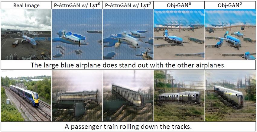
concatenated tensor through one up-sampling layer and sev-
eral residual layers to generate a higher-resolution image.
Grid attention vs. object-driven attention. The process
to compute the patch-wise context vectors above is the tra-
ditional grid attention mechanism used in AttnGAN [29].
                                    pat
Note that its attention weights βj,i    and context vector cpat
                                                             j
are useful only when the hidden feature hpat j in the G0 stage
correctly captures the content to be drawn in patch j. This
essentially assumes that the generation in the G0 stage al-
ready captures a rough sketch (semantic layout). This as-
sumption is valid for simple datasets like birds [29], but
fails for complex datasets like COCO [15] where the gen-
erated low-resolution image x    b0 typically does not have a
meaningful layout. In this case, the grid attention is even
harmful, because patch-wise context vector is attended to a
wrong word and thus generate the texture associated with
that wrong word. This may be the reason why AttnGAN’s
generated image contains scattered patches of realistic tex-                       Figure 5: Object-wise discriminator.
ture but overall is semantically not meaningful; see Fig. 1
for example. Similar phenomenon is also observed in Deep-
                                                                                        ppix = Dpix (Enc(x, M )),                   (9)
Dream [20]. On the contrary, in our object-driven attention,
                         obj
the attention weights βt,i   and context vector cobj
                                                  t rely on the
             g
class label lt of the bounding box and are independent of            where we first concatenate the image x and shapes M in the
the generation in the G0 stage. Therefore, the object-wise           channel dimension, and then extracts patch-wise features
context vectors are always helpful to generate images that           by another convolutional feature extractor Enc. The proba-
are consistent with the pre-generated semantic layout. An-           bilities ppix determine whether the patch is consistent with
                                                                                                                           pat
other benefit of this design is that the context vector cobj
                                                         t can       the given shape. Our patch-wise discriminators Duncond.     ,
                                                                       pat         pix
also be used in the discriminator, as we present in § 3.2.2.         Dtext and D resembles the PatchGAN [11] for the image-
                                                                     to-image translation task. Compared with the global dis-
3.2.2   Discriminators                                               criminators in AttnGAN [29], the patch-wise discriminators
                                                                     not only reduce the model size and thus enable generating
We design patch-wise and object-wise discriminators to               higher resolution images, but also increase the quality of
train the attentive multi-stage generator above. Given a             generated images; see Table 1 for experimental evidence.
patch from uniformly-partitioned image patches determined
by the uniform down-sampling structure of CNN, the patch-            Object-wise discriminators. Given an image x, bounding
wise discriminator is trying to determine whether this patch         boxes of objects B1:T and their shapes M , we propose the
is realistic or not (unconditional) and whether this patch           following object-wise discriminators:
is consistent with the sentence description or not (condi-
tional). Given a bounding box and the class label of the                            {hobj T
                                                                                      t }t=1 =FastRCNN(x, M, B1:T ),
object within it, the object-wise discriminator is trying to           pobj,un
                                                                        t
                                                                                  obj
                                                                               = Duncond. (hobj
                                                                                            t ),     pobj,con
                                                                                                      t        = Dobj (hobj  g obj
                                                                                                                        t , et , ct ).
determine whether this region is realistic or not (uncondi-                                                                         (10)
tional) and whether this region is consistent with the sen-          Here, we first concatenate the image x and shapes M
tence description and given class label or not (conditional).        and extract a region feature vector hobj    t for each bounding
Patch-wise discriminators. Given an image-sentence pair              box through a Fast R-CNN model [4] with an ROI-align
x, ē (ē is the sentence vector), the patch-wise unconditional      layer [7]; see Fig. 5(a). Then similar to the patch-wise dis-
and text discriminator can be written as                             criminator (8), the unconditional (conditional) probabilities
            pat                                 pat                  pobj,un
                                                                       t     ( pobj,con
                                                                                t       ) determine whether the t’th object is real-
 ppat,un = Duncond. (Enc(x)),     ppat,con = Dtext  (Enc(x), ē),
                                                                     istic (consistent with its class label egt and its text context
                                                               (8)
                                                                     information cobj                                   g
                                                                                     t ) or not; see Fig. 5(b). Here, et is the GloVe
where Enc is a convolutional feature extractor that extracts                                                  obj
                                   pat
patch-wise features, Duncond. ( Dtext   ) determine whether the      embedding of the class label and ct is its text context in-
patch is realistic (consistent with the text description) or not.    formation defined in (3).
Shape discriminator. In a similar manner, we have our                   All discriminators are trained by the traditional cross en-
patch-wise shape discriminator                                       tropy loss [5].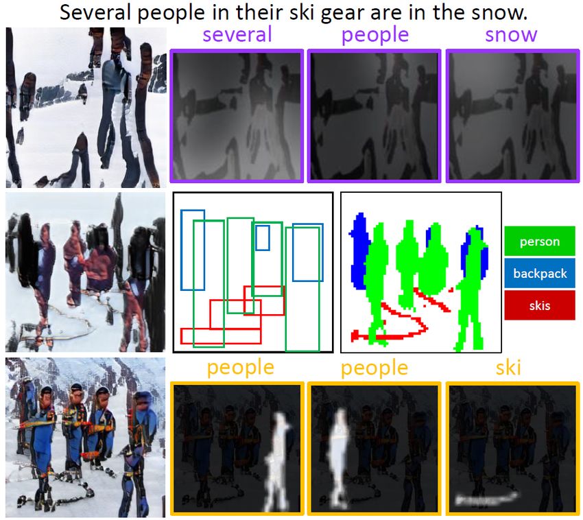
3.2.3 Loss function for the image generator Table 1: The quantitative experiments. Methods marked with 0, 1
and 2 respectively represent experiments using the predicted boxes
The generator’s GAN loss is a weighted sum of these dis- and shapes, the ground-truth boxes and predicted shapes, and the
criminators’ loss, i.e., ground-truth boxes and shapes. We use bold, ∗, and ∗∗ to high-
light the best performance under these three settings, respectively.
T The results of methods marked with † are those reported in the
λobj X obj,un
LGAN (G) = − log pt + log pobj,con original papers. ↑ (↓) means the higher (lower), the better.
t
T t=1
| {z } | {z }
obj uncond. loss obj cond. loss Methods Inception ↑ FID ↓ R-prcn (%) ↑
Obj-GAN0
27.37 ± 0.22 25.85 86.20 ± 2.98
pat
N Obj-GAN1 27.96 ± 0.39∗ 24.19∗ 88.36 ± 2.82
1 X pat,un
− log p + λtxt log ppat,con + λpix log ppix
j . Obj-GAN2 29.89 ± 0.22∗∗ 20.75∗∗
89.59 ± 2.67
N pat j=1 | {zj } | {z
j
} | {z } P-AttnGAN w/ Lyt0 18.84 ± 0.29 59.02 65.71 ± 3.74
uncond. loss text cond. loss shape cond. loss P-AttnGAN w/ Lyt1 19.32 ± 0.29 54.96 68.40 ± 3.79
P-AttnGAN w/ Lyt2 20.81 ± 0.16 48.47 70.94 ± 3.70
Here, T is the number of bounding boxes, N pat is the num- P-AttnGAN 26.31 ± 0.43 41.51 86.71 ± 2.97
Obj-GAN w/ SN0 26.97 ± 0.31 29.07 86.84 ± 2.82
ber of regular patches, (λobj , λtxt , λpix ) are the weights of the Obj-GAN w/ SN1 27.41 ± 0.17 27.26 88.70 ± 2.65∗
object-wise GAN loss, patch-wise text conditional loss and Obj-GAN w/ SN2 28.75 ± 0.32 23.37 89.97 ± 2.56∗∗
patch-wise shape conditional loss, respectively. We tried Reed et al. [23]† 7.88 ± 0.07 n/a n/a
StackGAN [32]† 8.45 ± 0.03 n/a n/a
combining our discriminators with the spectral normalized AttnGAN [29] 23.79 ± 0.32 28.76 82.98 ± 3.15
projection discriminator [18, 19], but did not see significant vmGAN [35]† 9.94 ± 0.12 n/a n/a
Sg2Im [12]† 6.7 ± 0.1 n/a n/a
performance improvement. We report performance of the
Infer [9]0 † 11.46 ± 0.09 n/a n/a
spectral normalized version in § 4.1 and provide model ar- Infer [9]1 † 11.94 ± 0.09 n/a n/a
chitecture details in § A. Infer [9]2 † 12.40 ± 0.08 n/a n/a
Obj-GAN-SOTA0 30.29 ± 0.33 25.64 91.05 ± 2.34
Combined with the deep multi-modal attentive similarity
Obj-GAN-SOTA1 30.91 ± 0.29 24.28 92.54 ± 2.16
model (DAMSM) loss introduced in [29], our final image Obj-GAN-SOTA2 32.79 ± 0.21 21.21 93.39 ± 2.08
generator’s loss is
a common evaluation metric for ranking retrieval results,
LG = LGAN + λDAMSM LDAMSM (11) to evaluate whether the generated image is well conditioned
on the given text description. More specifically, given a pre-
where λdamsm is a hyper-parameter to be tuned. Here, trained image-to-text retrieval model, we use generated im-
the DAMSM loss is a word level fine-grained image-text ages to query their corresponding text descriptions. First,
matching loss computed, which will be elaborated in § A. given generated image x b conditioned on sentence s and
Based on the experiments on a held-out validation set, we 99 random sampled sentences {s0i : 1 ≤ i ≤ 99}, we
set the hyperparameters in this section as: λobj = 0.1, λtxt = rank these 100 sentences by the pre-trained image-to-text
0.1, λpix = 1 and λdamsm = 100. retrieval model. If the ground truth sentence s is ranked
highest, we count this a success retrieval. For all the im-
Remark 3.1. Both the patch-wise and object-wise discrim-
ages in the test dataset, we perform this retrieval task once
inators can be applied to different stages in the generation.
and finally count the percentage of success retrievals as the
We apply the patch-wise discriminator for every stage of the
R-precision score.
generation, following [33, 11], but only apply the object-
wise discriminator at the final stage. It is important to point out that none of these quanti-
tative metrics are perfect. Better metrics are required to
evaluate image generation qualities in complicated scenes.
4. Experiments
In fact, the Inception score completely fails in evaluat-
Dataset. We use the COCO dataset [15] for evaluation. ing the semantic layout of the generated images. The R-
It contains 80 object classes, where each image is associ- precision score depends on the pre-trained image-to-text re-
ated with object-wise annotations (i.e., bounding boxes and trieval model it uses, and can only capture the aspects that
shapes) and 5 text descriptions. We use the official 2014 the retrieval model is able to capture. The pre-trained model
train (over 80K images) and validation (over 40K images) we use is still limited in capturing the relations between ob-
splits for training and test stages, respectively. jects in complicated scenes, so is our R-precision score.
Evaluation metrics. We use the Inception score [25] and Quantitative evaluation. We compute these three metrics
Fréchet inception distance (FID) [8] score as the quantita- under two settings for the full validation dataset.
tive evaluation metrics. In our experiments, we found that Qualitative evaluation. Apart from the quantitative evalua-
Inception score can be saturated, even over-fitted, while FID tion, we also visualize the outputs of all ablative versions of
is a more robust measure and aligns better with human qual- Obj-GAN and the state-of-the-art methods (i.e., [29]) whose
itative evaluation. Following [29], we also use R-precision, pre-trained models are publicly available.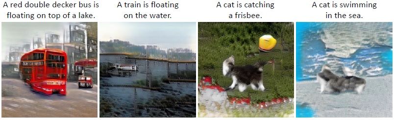
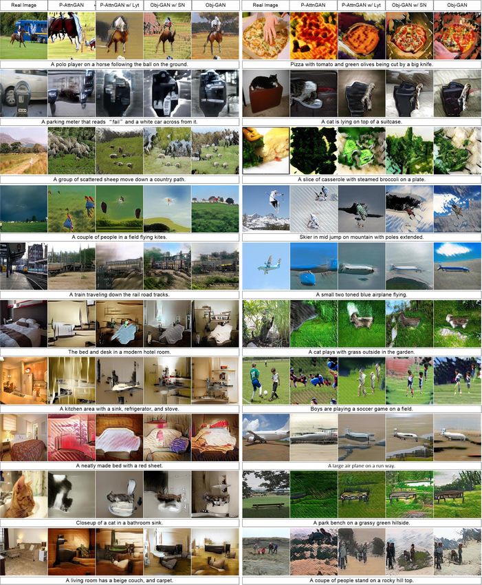
Figure 6: The overall qualitative comparison. All images are generated without the usage of any ground-truth information.
4.1. Ablation study                                                   functions: P-AttnGAN w/ Lyt uses the DAMSM loss in (11)
                                                                      to penalize the mismatch between the generated images and
   In this section, we first evaluate the effectiveness of the
                                                                      the input text descriptions, while [9] uses the perceptual loss
object-driven attention. Next, we compare the object-driven
                                                                      to penalize the mismatch between the generated images and
attention mechanism with the grid attention mechanism.
                                                                      the ground-truth images. As shown in Table 1, P-AttnGAN
Then, we evaluate the impact of the spectral normalization
                                                                      w/ Lyt yields higher Inception score than [9] does.
for Obj-GAN. We use Fig. 6 and the higher half of Table 1 to
present the comparison among different ablative versions of               We compare Obj-GAN with P-AttnGAN w/ Lyt under
Obj-GAN. Note that all ablative versions have been trained            three settings, with each corresponding to a set of condi-
with batch size 16 for 60 epochs. In addition, we use the             tional layout input, i.e., the predicted boxes & shapes, the
lower half of Table 1 to show the comparison between Obj-             ground-truth boxes & predicted boxes, and the ground-truth
GAN and previous methods. Finally, we validated the Obj-              boxes & shapes. As presented in Table 1, Obj-GAN con-
GAN’s generalization ability on the novel text descriptions.          sistently outperforms P-AttnGAN w/ Lyt on all three met-
Object-driven attention. To evaluate the efficacy of the              rics. In Fig. 7, we use the same layout as the conditional
object-driven attention mechanism, we implement a base-               input, and compare the visual quality of their generated im-
line, named P-AttnGAN w/ Lyt, by disabling the object-                ages. An interesting phenomenon shown in Fig. 7 is that
driven attention mechanism in Obj-GAN. In essence, P-                 both the foreground objects (e.g., airplane and train) and the
AttnGAN w/ Lyt can be considered as an improved version               background (e.g., airport and trees) textures synthesized by
of AttnGAN with the patch-wise discriminator (abbreviated             Obj-GAN are much richer and smoother than those using
as the prefix “P-” in name) and the modules (e.g., shape              P-AttnGAN w/ Lyt. The effectiveness of the object-driven
discriminator) for handling the conditional layout (abbre-            attention for the foreground objects is easy to understand.
viated as “Lyt”). Moreover, it can also be considered as a            The benefits for the background textures using the object-
modified implementation of [9], which resembles their two-            driven attention mechanism is probably due to the fact that
step (layout-image) generation. Note that there are three             it implicitly provides stronger signal that distinguishes the
key differences between P-AttnGAN w/ Lyt and [9]: (i)                 foreground. As such, the image generator may have richer
P-AttnGAN w/ Lyt has a multi-stage image generator that               guidance and clearer emphasis when synthesizing textures
gradually increases the generated resolution and refines the          for a certain region.
generated images, while [9] has a single-stage image gen-             Grid attention vs. object-driven attention. We compare
erator. (ii) With the help of the grid attentive module, P-           Obj-GAN with P-AttnGAN herein, so as to compare the
AttnGAN w/ Lyt is able to utilize the fine-grained word-              effects of the object-driven and the grid attention mecha-
level information, while [9] conditions on the global sen-            nisms. In Fig. 8, we show the generated image of each
tence information. (iii) The third difference lies in their loss      method as well as the corresponding attention maps aligned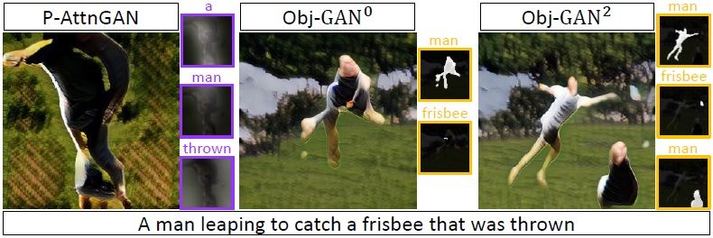
Figure 9: Generated images for novel descriptions.
                                                                 more results and discussions in § A.
                                                                 Comparison with previous methods. To compare Obj-
  Figure 7: Qualitative comparison with P-AttnGAN w/ Lyt.        GAN with the previous methods, initialized by the Obj-
                                                                 GAN models in the ablation study, we trained Obj-GAN-
                                                                 SOTA with batch size 64 for 10 more epochs. In order
                                                                 to evaluate AttnGAN on FID, we conducted the evalua-
                                                                 tion on the officially released pre-trained model. Note that
                                                                 the Sg2Im [12] focuses on generating images from scene
                                                                 graphs and conducted the evaluation on a different split of
                                                                 COCO. However, we still included Sg2Im’s results to re-
Figure 8: Qualitative comparison with P-AttnGAN. The attention   flect the broader context of the related topic. As shown in
maps of each method are shown beside the generated image.        Table 1, Obj-GAN-SOTA outperforms all previous meth-
                                                                 ods significantly. We notice that the increment of batch size
on the right side. In a grid attention map, the brightness of    does boost the Inception score and R-precision, but does
a region reflects how much this region attended to the word      not improve FID. The possible explanation is: with a larger
above the map. As for the object-driven attention map, the       batch size, the DAMSM loss (a ranking loss in essence) in
word above each attention map is the most attended word by       (11) plays a more important role and improves Inception
the highlighted object. The highlighted region of an object-     and R-precision, but it does not focus on reducing FID be-
driven attention map is the object shape.                        tween the generated images and the real ones.
    As analyzed in § 3.2.1, the reliability of grid attention    Generalization ability. We further investigate if Obj-GAN
weights depends on the quality of the previous layer’s im-       just memorizes the scenarios in COCO or it indeed learns
age region features. This makes the grid attention unreliable    the relations between the objects and their surroundings.
sometimes, especially for complex scenes. For example,           To this end, we compose several descriptions which reflect
the grid attention weights in Fig. 8 are unreliable because      novel scenarios that are unlikely to happen in the real-world,
they are scattered (e.g., the attention map for “man”) and       e.g., a decker bus is floating on top of a lake, or a cat is
inaccurate. However, this is not a problem for the object-       catching a frisbee. We use Obj-GAN to synthesize images
driven attention mechanism, because its attention weights        for these rare scenes. The results in Fig. 9 further demon-
are directly calculated from embedding vectors of words          strate the good generalization ability of Obj-GAN.
and class labels and are independent of image features.
Moreover, as shown in Fig. 4 and Equ. (6), the impact re-
                                                                 5. Conclusions
gion of the object-driven attention context vector is bounded        In this paper, we have presented a multi-stage Object-
by the object shapes, which further enhances its semantics       driven Attentive Generative Adversarial Networks (Obj-
meaningfulness. As a result, the instance-driven attention       GANs) for synthesizing images with complex scenes from
significantly improves the visual quality of the generated       the text descriptions. With a novel object-driven attention
images, as demonstrated in Fig. 8. Moreover, the perfor-         layer at each stage, our generators are able to utilize the
mance can be further improved if the semantic layout gen-        fine-grained word/object-level information to gradually re-
eration is improved. In the extreme case, Obj-GAN based          fine the synthesized image. We also proposed the Fast R-
on ground truth layout (Obj-GAN2 ) has the best visual qual-     CNN based object-wise discriminators, each of which is
ity (the rightmost column of Fig. 8) and the best quantitative   paired with a conditional input of the generator and provides
evaluation (Table 1).                                            object-wise discrimination signal for that condition. Our
Obj-GAN w/ SN vs. Obj-GAN. We present the compari-               Obj-GAN significantly outperforms previous state-of-the-
son between the cases with or without spectral normaliza-        art GAN models on various metrics on the large-scale chal-
tion in the discriminators in Table 1 and Fig. 6. We observe     lenging COCO benchmark. Extensive experiments demon-
that there is no obvious improvement on the visual qual-         strate the effectiveness and generalization ability of Obj-
ity, but slightly worse on the quantitative metrics. We show     GAN on text-to-image generation for complex scenes.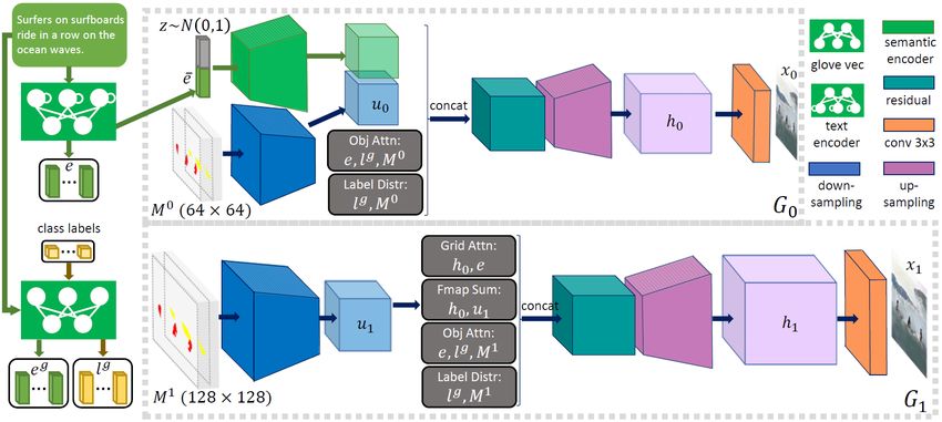
References                                                            [22] S. Reed, Z. Akata, S. Mohan, S. Tenka, B. Schiele, and
                                                                           H. Lee. Learning what and where to draw. In NIPS, 2016.
 [1] P. Anderson, X. He, C. Buehler, D. Teney, M. Johnson,
                                                                      [23] S. Reed, Z. Akata, X. Yan, L. Logeswaran, B. Schiele, and
     S. Gould, and L. Zhang. Bottom-up and top-down attention
                                                                           H. Lee. Generative adversarial text-to-image synthesis. In
     for image captioning and vqa. CVPR, 2018.
                                                                           ICML, 2016.
 [2] D. Bahdanau, K. Cho, and Y. Bengio.               Neural ma-
     chine translation by jointly learning to align and translate.    [24] S. E. Reed, A. van den Oord, N. Kalchbrenner, S. G. Col-
     arXiv:1409.0473, 2014.                                                menarejo, Z. Wang, Y. Chen, D. Belov, and N. de Fre-
 [3] E. L. Denton, S. Chintala, A. Szlam, and R. Fergus. Deep              itas. Parallel multiscale autoregressive density estimation.
     generative image models using a laplacian pyramid of adver-           In ICML, 2017.
     sarial networks. In NIPS, 2015.                                  [25] T. Salimans, I. J. Goodfellow, W. Zaremba, V. Cheung,
 [4] R. B. Girshick. Fast R-CNN. In ICCV, 2015.                            A. Radford, and X. Chen. Improved techniques for training
 [5] I. J. Goodfellow, J. Pouget-Abadie, M. Mirza, B. Xu,                  gans. In NIPS, 2016.
     D. Warde-Farley, S. Ozair, A. C. Courville, and Y. Bengio.       [26] A. van den Oord, N. Kalchbrenner, O. Vinyals, L. Espeholt,
     Generative adversarial nets. In NIPS, 2014.                           A. Graves, and K. Kavukcuoglu. Conditional image genera-
 [6] K. Gregor, I. Danihelka, A. Graves, D. J. Rezende, and                tion with pixelcnn decoders. In NIPS, 2016.
     D. Wierstra. DRAW: A recurrent neural network for image          [27] A. Vaswani, N. Shazeer, N. Parmar, J. Uszkoreit, L. Jones,
     generation. In ICML, 2015.                                            A. N. Gomez, L. Kaiser, and I. Polosukhin. Attention is all
 [7] K. He, G. Gkioxari, P. Dollár, and R. B. Girshick. Mask              you need. NIPS, 2017.
     R-CNN. In ICCV, 2017.
                                                                      [28] K. Xu, J. Ba, R. Kiros, K. Cho, A. C. Courville, R. Salakhut-
 [8] M. Heusel, H. Ramsauer, T. Unterthiner, B. Nessler,                   dinov, R. S. Zemel, and Y. Bengio. Show, attend and tell:
     G. Klambauer, and S. Hochreiter. GANs trained by a two                Neural image caption generation with visual attention. In
     time-scale update rule converge to a nash equilibrium. NIPS,          ICML, 2015.
     2017.
                                                                      [29] T. Xu, P. Zhang, Q. Huang, H. Zhang, Z. Gan, X. Huang, and
 [9] S. Hong, D. Yang, J. Choi, and H. Lee. Inferring semantic
                                                                           X. He. Attngan: Fine-grained text to image generation with
     layout for hierarchical text-to-image synthesis. CVPR, 2018.
                                                                           attentional generative adversarial networks. CVPR, 2018.
[10] Q. Huang, P. Zhang, D. O. Wu, and L. Zhang. Turbo learning
     for captionbot and drawingbot. In NeurIPS, 2018.                 [30] Z. Yang, X. He, J. Gao, L. Deng, and A. J. Smola. Stacked
[11] P. Isola, J.-Y. Zhu, T. Zhou, and A. A. Efros. Image-to-image         attention networks for image question answering. In CVPR,
     translation with conditional adversarial networks. In CVPR,           2016.
     2017.                                                            [31] H. Zhang, I. Goodfellow, D. Metaxas, and A. Odena. Self-
[12] J. Johnson, A. Gupta, and L. Fei-Fei. Image generation from           attention generative adversarial networks. arXiv preprint
     scene graphs. In CVPR, 2018.                                          arXiv:1805.08318, 2018.
[13] C. Ledig, L. Theis, F. Huszar, J. Caballero, A. Aitken, A. Te-   [32] H. Zhang, T. Xu, H. Li, S. Zhang, X. Wang, X. Huang, and
     jani, J. Totz, Z. Wang, and W. Shi. Photo-realistic single im-        D. Metaxas. Stackgan: Text to photo-realistic image synthe-
     age super-resolution using a generative adversarial network.          sis with stacked generative adversarial networks. In ICCV,
     In CVPR, 2017.                                                        2017.
[14] K. Lee, X. Chen, G. Hua, H. Hu, and X. He. Stacked cross         [33] H. Zhang, T. Xu, H. Li, S. Zhang, X. Wang, X. Huang, and
     attention for image-text matching. ECCV, 2018.                        D. N. Metaxas. Stackgan++: Realistic image synthesis with
[15] T.-Y. Lin, M. Maire, S. Belongie, J. Hays, P. Perona, D. Ra-          stacked generative adversarial networks. TPAMI, 2018.
     manan, P. Dollr, and C. L. Zitnick. Microsoft coco: Common       [34] S. Zhang, H. Dong, W. Hu, Y. Guo, C. Wu, D. Xie, and
     objects in context. In ECCV, 2014.                                    F. Wu. Text-to-image synthesis via visual-memory creative
[16] S. Ma, J. Fu, C. W. Chen, and T. Mei. DA-GAN: Instance-               adversarial network. In PCM, 2018.
     level image translation by deep attention generative adver-
                                                                      [35] S. Zhang, H. Dong, W. Hu, Y. Guo, C. Wu, D. Xie, and
     sarial networks. In CVPR, 2018.
                                                                           F. Wu. Text-to-image synthesis via visual-memory creative
[17] E. Mansimov, E. Parisotto, L. J. Ba, and R. Salakhutdinov.
                                                                           adversarial network. In PCM, 2018.
     Generating images from captions with attention. In ICLR,
     2016.
[18] T. Miyato, T. Kataoka, M. Koyama, and Y. Yoshida. Spec-          A. Appendix
     tral normalization for generative adversarial networks. ICLR,
     2018.                                                            A.1. Obj-GAN vs. the ablative versions
[19] T. Miyato and M. Koyama. cgans with projection discrimi-
     nator. ICLR, 2018.                                                  In this section, we show more images generated by our
[20] A. Mordvintsev, C. Olah, and M. Tyka. Deep dream, 2015,          Obj-GAN and its ablative versions on the COCO dataset.
     2017.                                                            In Fig. 10 and Fig. 11, we provide more comparisons as the
[21] A. Radford, L. Metz, and S. Chintala. Unsupervised repre-        complementary for Fig. 6. It can be found that there are no
     sentation learning with deep convolutional generative adver-     obvious improvement on the visual quality when using the
     sarial networks. In ICLR, 2016.                                  spectral normalization.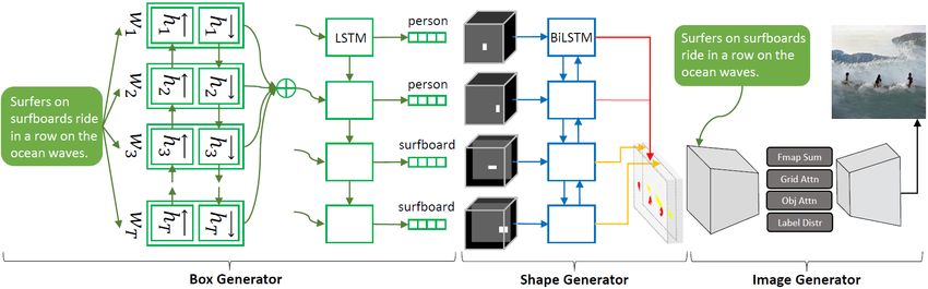
Figure 10: The overall qualitative comparison.

A.2. Visualization of attention maps                             A.3. Results based on the ground-truth layout
                                                                    We show the results generated by Obj-GAN based on the
   In Fig. 12, we visualize attention maps generated by P-       ground-truth layout in Fig. 13, Fig. 14 and Fig. 15.
AttnGAN and Obj-GAN as the complementary for Fig. 8.
Figure 11: The overall qualitative comparison.
Figure 12: Qualitative comparison with P-AttnGAN. The attention maps of each method are shown beside the generated image.
(1) A glass table with a bottle (2) A train sitting on some (3) Soccer player wearing green (4) A kitchen with a very messy
and glass of wine next to a chair. tracks next to a sidewalk. and orange hitting soccer ball. counter space.

(5) The people are on the beach (6) A jet airliner waits its turn (7) Two cows are grazing in a (8) A small lightweight airplane
getting ready to surf.          on the runway.                    dirt field.                   flying through the sky.

(9) A cow running in a field next (10) Two people go into the wa- (11) A man in a helmet jumps a (12) A giraffe is standing all
to a dog.                         ter with their surfboards.      snowboard.                     alone in a grassy area.

(13) The black dog is staring at (14) A bunch of sheep are (15) A bench sitting on top of a (16) A polar bear playing in the
the cat.                         standing in a field.      lush green hillside.             water at a wild life enclosure.

                                      Figure 13: Results based on the ground-truth layout.
(1) A man on a soccer field next (2) A dog sitting on a bench in (3) A black cat drinking water (4) A cat laying on a TV in the
to a ball. front of a garden. out of a water faucet. middle of the room.
(5) Four people on skis below a (6) A man in outdoor winter (7) A orange before and after it (8) A dog running with a frisbee
mountain taking a picture. clothes holds a snowboard. was cu. in its mouth.
(9) A woman and a dog tussle (10) Man in a wetsuit on top of (11) A white ship sails in the (12) A couple of men standing
over a frisbee. a blue and white surfboard. blue ocean water. next to dogs near water.
(13) A man on a motorcycle in (14) A group of people riding (15) A hipster wearing flood (16) A black dog holding a fris-
a carport. horses on a beach. pants poses with his skateboard. bee in its mouth.
Figure 14: Results based on the ground-truth layout.(1) A big boat on the water near (2) All the horses in the pen are (3) A man riding a bike down (4) A bathroom with a sink and
the shore. grazing. the middle of a street. a toilet.
(5) A yellow school bus parked (6) A group of cows graze on (7) A ship is sailing across an (8) Three skiers posing for a
near a tree. some grass. ocean filled with waves. picture on the slope.
(9) A large green bus approach- (10) A close view of a pizza, (11) A cat is looking at a televi- (12) Three white sinks in a bath-
ing a bus stop. and a mug of beer. sion displaying a dog in a cage. room under mirrors.
(13) Three cranes standing on (14) A bear lying on a rock in (15) Two bottles of soda sit near (16) Someone on a snowboard
one leg in the water. its den, looking upward. a sandwich. coming to a stop.
Figure 15: Results based on the ground-truth layout.A.4. Bi-LSTM text encoder, DAMSM and R- However, it is difficult to obtain manual annotations. Ac-
precision tually, many words relate to concepts that may not easily be
visually defined, such as open or old. One possible solution
We use the deep attentive multi-modal similarity model
is to learn word-image correspondence in a semi-supervised
(DAMSM) proposed in [29], which learns a joint embed-
manner, in which the only supervision is the correspon-
ding of the image regions and words of a sentence in a com-
dence between the entire image and the whole text descrip-
mon semantic space. The fine-grained conditional loss en-
tion (a sequence of words).
forces the sub-region of the generated image to match the
We can first calculate the similarity matrix between all
corresponding word in the sentence.
possible pairs of word and image region by Eq. (13),
Bi-LSTM text encoder serves as the text encoder for
both DAMSM and the box generator (see § A.5). Bi-LSTM s = ėT v, (13)
text encoder is a bi-directional LSTM that extracts seman- T ×289
tic vectors from the text description. In the Bi-LSTM, each where s ∈ R and si,j means the similarity between
word corresponds to two hidden states, one for each direc- the ith word and the j th image region.
tion. Thus, we concatenate its two hidden states to represent Generally, a sub-region of the image is described by none
the semantic meaning of a word. The feature matrix of all or several words of the text description, and it is not likely
words is indicated by ė ∈ RD×Ts . Its ith column ėi is the to be described by the whole sentence. Therefore, we nor-
feature vector for the ith word. D is the dimension of the malize the similarity matrix by Eq. (14),
word vector and Ts is the number of words. Meanwhile, the exp(si,j )
last hidden states of the bi-directional LSTM are concate- si,j = PT −1 (14)
k=0 exp(sk,j )
nated to be the global sentence vector, denoted by eb ∈ RD .
We present the network architectures for the Bi-LSTM text Second, we build an attention model to compute a con-
encoder in Table 2. text vector for each word (query). The context vector ci is
The image encoder is a convolutional neural network a dynamic representation of image regions related to the ith
that maps images to semantic vectors. The intermediate lay- word of the text description. It is computed as the weighted
ers of the CNN model learns local features of different re- sum over all visual feature vectors,
gions of the image, while the later layers learn global fea- 288
X
tures of the image. More specifically, the image encoder ci = αj vj , (15)
is built upon Inception-v3 model pre-trained on ImageNet. j=0
We first rescale the input image to be 299×299 pixels. And
then, we extract the local feature matrix f ∈ R768×289 where we define the weight αj via Eq. (16),
(reshaped from 768×17×17) from “mixed 6e” layer of exp(γ1 si,j )
Inception-v3. Each column of f is the feature vector of a αj = P288 (16)
k=0 exp(γ1 si,k )
local image region. 768 is the dimension of the local fea-
ture vector, and 289 is the number of regions in the im- Here, γ1 is a factor that decides how much more attention is
age. Meanwhile, the global feature vector f ∈ R2048 is paid to features of its relevant regions when computing the
extracted from the last average pooling layer of Inception- context vector for a word.
v3. Finally, we convert the image features to the common Finally, we define the relevance between the ith word
semantic space of text features by adding a new layer per- and the image using the cosine similarity between ci and
ceptron as shown in Eq. (12), ėi , i.e., R(ci , ėi ) = (cTi ėi )/(||ci ||||ėi ||). The relevance be-
tween the entire image (Q) and the whole text description
v = Wf; v = W f, (12) (U) is computed by Eq. (17),
D×289 th
where v ∈ R and its i column vi is the visual fea- −1
TX γ1
ture vector for the ith image region; v ∈ RD is the visual R(Q, U ) = log exp(γ2 R(ci , ėi ))
2
, (17)
feature vector for the whole image. While vi is the local im- i=1
age feature vector that corresponds to the word embedding,
where γ2 is a factor that determines how much to magnify
v is the global feature vector that is related to the sentence
the importance of the most relevant word-image pair. When
embedding. D is the dimension of the multimodal (i.e., im- −1
γ2 → ∞, R(Q, U ) approximates to maxTi=1 R(ci , ėi ).
age and text modalities) feature space. For efficiency, all pa-
For a text-image pair, we can compute the posterior prob-
rameters in layers built from Inception-v3 model are fixed,
ability of the text description (U ) being matching with the
and the parameters in newly added layers are jointly learned
image (Q) via,
with the rest of networks.
The fine-grained conditional loss is designed to learn exp(γ3 R(Q, U ))
P (U |Q) = P , (18)
the correspondence between image regions and words. 0
U 0 ∈U exp(γ3 R(Q, U ))where γ3 is a smoothing factor determined by experiments. box of the t-th object as Bt = (bxt , byt , bw h
t , bt , lt ). Then, we
U denotes a minibatch of M text descriptions, in which only formulate the joint probability of sampling Bt from the box
one description U + matches the image Q. Thus, for each generator as
image, there are M − 1 mismatching text descriptions. The
p(bxt , byt , bw h x y w h
t , bt , lt ) = p(lt )p(bt , bt , bt , bt |lt ). (22)
objective function is to learn the model parameters Λ by
minimizing the negative log posterior probability that the We implement p(lt ) as a categorical distribution, and im-
images are matched with their corresponding text descrip- plement p(bxt , byt , bw h
t , bt |lt ) as a mixture of quadravariate
tions (ground truth), Gaussians. As described in [9], in order to reduce the pa-
Y rameter space, we decompose the box coordinate probabil-
Lw1 (Λ) = − log P (U + |Q), (19) ity as p(bxt , byt , bw h x y w h x y
t , bt |lt ) = p(bt , bt |lt )p(bt , bt |bt , bt , lt ),
Q∈Q and approximate it with two bivariate Gasussian mixtures
by
where ‘w’ stands for “word”.
K
Symmetrically, we can compute, X
p(bxt , byt |lt ) = xy
πt,k N (bxt , byt ; µxy xy
t,k , Σt,k ),
Y
Lw
2 (Λ) = − log P (Q+ |U ), (20) k=1
K
U ∈U h x y
X
p(bw
t , bt |bt , bt , lt ) =
wh
πt,k N (bw h wh wh
t , bt ; µt,k , Σt,k ).
where P (Q|U ) = P exp(γ3 R(Q,U ))0 . k=1
Q0 ∈Q exp(γ3 R(Q ,U )) (23)
If we redefine Eq. (17) by R(Q, U ) = v T eb / ||v||||b
e||
and substitute it to Eq. (18), Eq. (19), Eq. (20), we can ob- In practice, as in [9], we implement the box generator within
tain loss functions Ls1 and Ls2 (where ‘s’ stands for “sen- a encoder-decoder framework. The encoder is the Bi-LSTM
tence”) using the sentence embedding eb and the global vi- text encoder as mentioned in § A.4. The Gaussian Mixture
sual vector v. Model (GMM) parameters for Eq. (22) are obtained from
The fine-grained conditional loss is defined via Eq. (21), the decoder LSTM outputs. Given text encoder’s final hid-
den state hEnc D
Ts ∈ R and output H
Enc
∈ RTs ×D , we initial-
LDAM SM = Lw w s s
1 + L2 + L1 + L2 (21) ize the decoder’s initial hidden state h0 with hEnc
Ts . As for
Enc
H , we use it to compute the contextual input zt for the
The DAMSM is pre-trained by minimizing LDAM SM us- decoder:
ing real image-text pairs. Since the size of images for pre- Ts
training DAMSM is not limited by the size of images that
X
zt = αi hEnc Enc
i , with αi = Wv · (Wα [ht−1 , hi ]),
can be generated, real images of size 299×299 are utilized. i=1
Furthermore, the pre-trained DAMSM can provide visually-
discriminative word features and a stable fine-grained con-
ditional loss for the attention generative network. (24)
The R-precision score. The DAMSM model is also where Wv is a learnable parameter, Wα is the parameter
used to compute the R-precision score. If there are R rele- of a linear transformation, and · and [·, ·] represent the dot
vant documents for a query, we examine the top R ranked product and concatenation operation, respectively.
retrieval results of a system, and find that r are relevant, Then, the calculation of GMM parameters are shown as
and then by definition, the R-precision (and also the preci- follows:
sion and recall) is r/R. More specifically, we use generated
[ht , ct ] = LSTM([Bt−1 , zt ]; [ht−1 , ct−1 ]), (25)
images to query their corresponding text descriptions. First,
l l
the image encoder and Bi-LSTM text encoder learned in our lt = W ht + b , (26)
pre-trained DAMSM are utilized to extract features of the θtxy
=W xy
[ht , lt ] + b , xy
(27)
generated images and the given text descriptions. Then, we
compute cosine similarities between the image features and θtwh =W wh
[ht , lt , bx , by ] + b wh
, (28)
the text features. Finally, we rank candidates text descrip- where θt·
= ·
[πt,1:K , µ·t,1:K , Σ·t,1:K ]
are the parameters for
tions for each image in descending similarity and find the GMM concatenated to a vector. We use the same Adam
top r relevant descriptions for computing the R-precision. optimizer and training hyperparameters (i.e., learning rate
0.001, β1 = 0.9, β2 = 0.999) as in [9].
A.5. Network architectures for semantic layout gen-
Shape generator. We implement the shape generator
eration
in [9] with almost the same architecture except the upsam-
Box generator. We design our box generator by improv- ple block. In [9], the upsample block is designed as [con-
ing the one in [9] to be attentive. We denote the bounding vtranspose 4 × 4 (pad 1, stride 2) - Instance Normalization- ReLU]. We discovered that the usage of convtranspose same hyperparameters. would lead to unstable training which is reflected by the We design the object-wise discriminators for small ob- frequent severe grid artifacts. To this end, we replace this jects and large objects, respectively. We specify that if the upsample block with that in our image generator (see Ta- maximum of width or height of an object is greater than ble 3) by switching the batch normalization to the instance one-third of the image size, then this object is large; other- one. wise, it is small. A.6. Network architectures for image generation A.7. Network architectures for spectral normalized We present the network architecture for image generators projection discriminators in Table 4 and the network architectures for discriminators We combine our discriminators above with the spectral in Table 5, Table 6 and Table 7. They are built with basic normalized projection discriminator in [18, 19]. The differ- blocks defined in Table 3. We set the hyperparameters of ence between the object-wise discriminator and the object- the network structures as: Ng = 48, Nd = 96, Nc = 80, wise spectral normalized projection discriminator is illus- Ne = 256, Nl = 50, m0 = 7, m1 = 3, and m2 = 3. trated in Figure 16. We present detailed network architec- We employ an Adam optimizer for the generators with tures of the spectral normalized projection discriminators in learning rate 0.0002, β1 = 0.5 and β2 = 0.999. For each Table 8, Table 9 and Table 10, with basic blocks defined in discriminator, we also employ an Adam optimizer with the Table 3.
Table 2: The architecture of Bi-LSTM text encoder.

            Layer Name                                                   Hyperparameters
            Embedding      num embeddings = vocab size, embedding dim = 300
            Dropout        prob = 0.5
            LSTM           input size = 300, hidden size ( D
                                                           2
                                                             ) = 128, num layers = 1, dropout prob = 0.5, bidirectional = True

Table 3: The basic blocks for architecture design. (“-” connects two consecutive layers; “+” means element-wise addition
between two layers.)

 Name                                                                               Operations / Layers
 Interpolating (k)              Nearest neighbor upsampling layer (up-scaling the spatial size by k)
                                Interpolating (2) - convolution 3 × 3 (stride 1, padding 1, decreasing ]channels to k) -
 Upsampling (k)
                                Batch Normalization (BN) - Gated Linear Unit (GLU).
                                In Gs: convolution 3 × 3 (stride 2, increasing ]channels to k) - BN - LeakyReLU.
 Downsampling (k)
                                In Ds, the convolutional kernel size is 4. In the first block of Ds, BN is not applied.
                                Convolution 4 × 4 (spectral normalized, stride 2, increasing ]channels to k) - BN - LeakyReLU.
 Downsampling w/ SN (k)
                                In the first block of Ds, BN is not applied.
 Concat                         Concatenate input tensors along the channel dimension.
                                Input + [Reflection Pad (RPad) 1 - convolution 3 × 3 (stride 1, doubling ]channels) -
 Residual
                                Instance Normalization (IN) - GLU - RPad 1 - convolution 3 × 3 (stride 1, keeping ]channels) - IN].
 FC                             At the beginning of Gs: fully connected layer - BN - GLU - reshape to 3D tensor.
 FC w/ SN (k)                   Fully connected layer (spectral normalized, changing ]channels to k).
 Outlogits                      Convolution 4 × 4 (stride 2, decreasing ]channels to 1) - sigmoid.
 Repeat (k × k)                 Copy a vector k × k times.
 Fmap Sum                       Summing the two input feature maps element-wisely.
 Fmap Mul                       Multiplying the two input feature maps element-wisely.
 Avg Pool (k)                   Average pooling along the k-th dimension.
                                In Gs: convolution 3 × 3 (stride 1, padding 1, changing ]channels to k) - Tanh.
 Conv 3 × 3 (k)
                                In Ds, convolution 3 × 3 (stride 1, padding 1, changing ]channels to k) - BN - LeakyReLU.
 Conv 4 × 4 w/ SN               Convolution 4 × 4 (spectral normalized, stride 2, keeping ]channels).
 Conv 1 × 1 w/ SN               Convolution 1 × 1 (spectral normalized, stride 1, decreasing ]channels to 1).
                                Conditioning augmentation that converts the sentence embedding eb to the conditioning vector e:
 F ca
                                fully connected layer - ReLU.
 F pat-attn                     Grid attention module. Refer to the paper for more details.
 F obj-attn                     Object-driven attention module. Refer to the paper for more details.
 F lab-distr                    Label distribution module. Refer to the paper for more details.
 Shape Encoder (k)              RPad 1 - convolution 3 × 3 (stride 1, decreasing ]channels to k) - IN - LeakyReLU.
 Shape Encoder w/ SN (k)        RPad 1 - convolution 3 × 3 (spectral normalized, stride 1, decreasing ]channels to k) - IN - LeakyReLU.
 ROI Encoder                    Convolution 4 × 4 (stride 1, padding 1, decreasing ]channels to Nd ∗ 4) - LeakyReLU.
 ROI Encoder w/ SN              Convolution 4 × 4 (spectral normalized, stride 1, padding 1, decreasing ]channels to Nd ∗ 4) - LeakyReLU.
 ROI Align (k)                  Pooling k × k feature maps for ROI.
Table 4: The structure for generators of Obj-GAN.
Stage Name Input Tensors Output Tensors
FC 100-dimensional z, and F ca 8 × 8 × 4Ng
Upsampling (2Ng ) 8 × 8 × 4Ng 16 × 16 × 2Ng
Upsampling (Ng ) 16 × 16 × 2Ng c (32 × 32 × Ng )
Shape Encoder ( 21 Ng ) M 0 (64 × 64 × Nc ) 64 × 64 × 12 Ng
G0 Downsampling (Ng ) 64 × 64 × 12 Ng u0 (32 × 32 × Ng )
Concat c, u0 , F obj-attn , F lab-distr 32 × 32 × (3Ng + Nl )
m0 Residual 32 × 32 × (3Ng + Nl ) 32 × 32 × (3Ng + Nl )
Upsampling (Ng ) 32 × 32 × (3Ng + Nl ) h0 (64 × 64 × Ng )
Conv 3 × 3 (3) h0 x0 (64 × 64 × 3)
Shape Encoder ( 21 Ng ) M 1 (128 × 128 × Nc ) 128 × 128 × 12 Ng
Downsampling (Ng ) 128 × 128 × 12 Ng u1 (64 × 64 × Ng )
Fmap Sum h0 , u1 h0 (64 × 64 × Ng )
G1 Concat F pat-attn , h0 , F obj-attn , F lab-distr 64 × 64 × (3Ng + Nl )
m1 Residual 64 × 64 × (3Ng + Nl ) 64 × 64 × (3Ng + Nl )
Upsampling (Ng ) 64 × 64 × (3Ng + Nl ) h1 (128 × 128 × Ng )
Conv 3 × 3 (3) h1 x1 (128 × 128 × 3)
Shape Encoder ( 21 Ng ) M 2 (256 × 256 × Nc ) 256 × 256 × 12 Ng
Downsampling (Ng ) 256 × 256 × 12 Ng u2 (128 × 128 × Ng )
Fmap Sum h1 , u2 h1 (128 × 128 × Ng )
G2 Concat F pat-attn , h1 , F obj-attn , F lab-distr 128 × 128 × (3Ng + Nl )
m2 Residual 128 × 128 × (3Ng + Nl ) 128 × 128 × (3Ng + Nl )
Upsampling (Ng ) 128 × 128 × (3Ng + Nl ) h2 (256 × 256 × Ng )
Conv 3 × 3 (3) h2 x2 (256 × 256 × 3)
Table 5: The structure for patch-wise discriminators of Obj-GAN. e is output by F ca
Stage Name Input Tensors Output Tensors
Downsampling (Nd ) x0 (64 × 64 × 3) 32 × 32 × Nd
Downsampling (2Nd ) 32 × 32 × Nd 16 × 16 × 2Nd
Downsampling (4Nd ) 16 × 16 × 2Nd 8 × 8 × 4Nd
D0 Downsampling (8Nd ) 8 × 8 × 4Nd h0 (4 × 4 × 8Nd )
Repeat (4 × 4) e (Ne ) 4 × 4 × Ne
Concat - Conv 3 × 3 (8Nd ) h0 , 4 × 4 × Ne he0 (4 × 4 × 8Nd )
Outlogits (unconditional loss) h0 1
Outlogits (conditional loss) he0 1
Downsampling (Nd ) x1 (128 × 128 × 3) 64 × 64 × Nd
Downsampling (2Nd ) 64 × 64 × Nd 32 × 32 × 2Nd
Downsampling (4Nd ) 32 × 32 × 2Nd 16 × 16 × 4Nd
D1 Downsampling (8Nd ) 16 × 16 × 4Nd h1 (8 × 8 × 8Nd )
Repeat (8 × 8) e (Ne ) 8 × 8 × Ne
Concat - Conv 3 × 3 (8Nd ) h1 , 8 × 8 × Ne he1 (8 × 8 × 8Nd )
Outlogits (unconditional loss) h1 3×3
Outlogits (conditional loss) he1 3×3
Downsampling (Nd ) x2 (256 × 256 × 3) 128 × 128 × Nd
Downsampling (2Nd ) 128 × 128 × Nd 64 × 64 × 2Nd
Downsampling (4Nd ) 64 × 64 × 2Nd 32 × 32 × 4Nd
D2 Downsampling (8Nd ) 32 × 32 × 4Nd h2 (16 × 16 × 8Nd )
Repeat (16 × 16) e (Ne ) 16 × 16 × Ne
Concat - Conv 3 × 3 (8Nd ) h2 , 16 × 16 × Ne he2 (16 × 16 × 8Nd )
Outlogits (unconditional loss) h2 7×7
Outlogits (conditional loss) he2 7×7You can also read