ANOMALY-BASED INTRUSION DETECTION USING CONVOLUTIONAL NEURAL NETWORKS FOR IOT DEVICES - ALBIN SÖDERSTRÖM
←
→
Page content transcription
If your browser does not render page correctly, please read the page content below
Master of Science in Engineering: Computer Security
June 2021

   Anomaly-based Intrusion Detection
  Using Convolutional Neural Networks
            for IoT Devices

                             Albin Söderström

  Faculty of Computing, Blekinge Institute of Technology, 371 79 Karlskrona, Sweden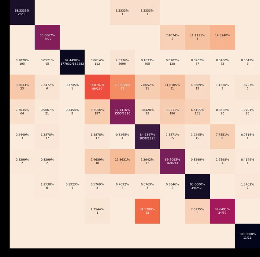
This thesis is submitted to the Faculty of Computing at Blekinge Institute of Technology in partial
fulfilment of the requirements for the degree of Master of Science in Engineering: Computer
Security. The thesis is equivalent to 20 weeks of full time studies.

The authors declare that they are the sole authors of this thesis and that they have not used
any sources other than those listed in the bibliography and identified as references. They further
declare that they have not submitted this thesis at any other institution to obtain a degree.

Contact Information:
Author:
Albin Söderström
E-mail: also15@student.bth.se

University advisor:
Emiliano Casalicchio
Department of Computer Science

Faculty of Computing                                Internet : www.bth.se
Blekinge Institute of Technology                    Phone    : +46 455 38 50 00
SE–371 79 Karlskrona, Sweden                        Fax      : +46 455 38 50 57
Abstract

Background. The rapid growth of IoT devices in homes put people at risk of cyber
attacks and the low power and computing capabilities in IoT devices make it difficult
to design a security solution for them. One method of preventing cyber attacks is
an Intrusion Detection System (IDS) that can identify incoming attacks so that an
appropriate action can be taken. Previous attempts have been made using machine
learning and deep learning however these attempts have struggled at detecting new
attacks.
Objectives. In this work we use a convolutional neural network IoTNet designed for
IoT devices to classify network attacks. In order to evaluate the use of deep learning
in intrusion detection systems on IoT.
Methods. The neural network was trained on the NF-UNSW-NB15-v2 dataset
which contains 9 different types of attacks. We used a method that transformed
the network flow data into RGB images which were fed to the neural network for
classification. We compared IoTNet to a basic convolutional neural network as a
baseline.
Results. The results show that IoTNet did not perform better at classifying network
attacks when compared to a basic convolutional neural network. It also showed that
both network had low precision for most classes.
Conclusions. We found that IoTNet is unfit to be used as an intrusion detection
system in the general case and that further research must be done in order to improve
the precision of the neural network.

Keywords: Internet of Things, Deep learning, Intrusion detection
Sammanfattning

Bakgrund. Den snabba tillväxten av IoT-enheter i hem utsätter folk för en risk av
cyberattacker och den låga effekten och datorkapaciteten i IoT-enheter gör det svårt
att utforma en säkerhetslösning för dem. En metod för att förhindra cyberattacker
är ett Intrusion Detection System (IDS) som kan identifiera inkommande attacker så
att en lämplig åtgärd kan vidtas. Tidigare forskning har gjorts med machine learning
och deep learning men dessa har haft svårt för att upptäcka nya attacker.
Syfte. I detta arbete använder vi ett convolutional neural network IoTNet ämnat
för IoT-enheter för att klassificera nätverksattacker. För att utvärdera användningen
av deep learning i intrångsdetekterningssystem på IoT-enheter.
Metod. Det neurala nätverket tränades på datasetet NF-UNSW-NB-v2 som in-
nehåller 9 olika typer av attacker. Vi använde en metod som transformerade nätverks-
flödesdata till RGB-bilder som matades till det neurala nätverket för klassificering.
Vi jämförde IoTNet med ett simpelt convolutional neural network som baslinje.
Resultat. Resultaten visade att IoTNet inte presterade bättre med att klassificera
nätverksattacker jämfört med ett simpelt convolutional neural network. Det visade
också att båda nätverken hade låg precision för de flesta klasser.
Slutsatser. Vi fann att IoTNet i allmänhet är olämpligt att användas som IDS
och att ytterligare forskning måste göras för att förbättra det neurala nätverkets
precision.

Nyckelord: Internet of Things, Deep learning, Intrusion detection

                                         iii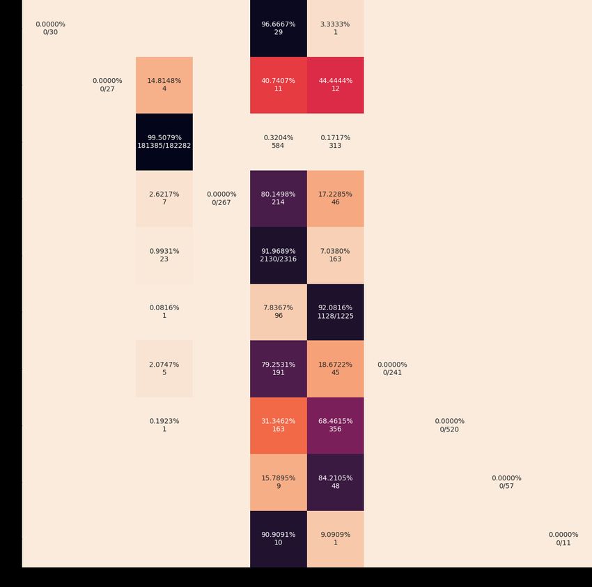
Acknowledgments

I’d like to thank my supervisor for letting me do this.

                                          v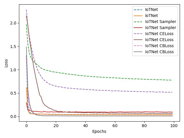
Contents

Abstract                                                                                                                           i

Sammanfattning                                                                                                                   iii

Acknowledgments                                                                                                                   v

1 Introduction                                                                                                                    1

2 Related Work                                                                                                                    3
      2.0.1 Background . . . . . . . . . . . . . . . . . . . . . . . . . . . .                                                    5

3 Method                                                                                                                          7
      3.0.1 Literature review . . . .        .   .   .   .   .   .   .   .   .   .   .   .   .   .   .   .   .   .   .   .   .    7
      3.0.2 UNSW-NB15 . . . . . .            .   .   .   .   .   .   .   .   .   .   .   .   .   .   .   .   .   .   .   .   .    8
      3.0.3 Data processing . . . . .        .   .   .   .   .   .   .   .   .   .   .   .   .   .   .   .   .   .   .   .   .    9
      3.0.4 Models . . . . . . . . . .       .   .   .   .   .   .   .   .   .   .   .   .   .   .   .   .   .   .   .   .   .   11
  3.1 Training . . . . . . . . . . . . .     .   .   .   .   .   .   .   .   .   .   .   .   .   .   .   .   .   .   .   .   .   13
      3.1.1 Hardware . . . . . . . .         .   .   .   .   .   .   .   .   .   .   .   .   .   .   .   .   .   .   .   .   .   13
      3.1.2 Hyperparameters . . . .          .   .   .   .   .   .   .   .   .   .   .   .   .   .   .   .   .   .   .   .   .   13
      3.1.3 Dataset imbalance . . .          .   .   .   .   .   .   .   .   .   .   .   .   .   .   .   .   .   .   .   .   .   14
      3.1.4 Classification experiment        .   .   .   .   .   .   .   .   .   .   .   .   .   .   .   .   .   .   .   .   .   15

4 Results and Analysis                                                                                                           17
  4.1 Training and validation . . . .    .   .   .   .   .   .   .   .   .   .   .   .   .   .   .   .   .   .   .   .   .   .   17
  4.2 Classification . . . . . . . . .   .   .   .   .   .   .   .   .   .   .   .   .   .   .   .   .   .   .   .   .   .   .   19
      4.2.1 Cross-entropy loss . . .     .   .   .   .   .   .   .   .   .   .   .   .   .   .   .   .   .   .   .   .   .   .   20
      4.2.2 Re-sampling . . . . . .      .   .   .   .   .   .   .   .   .   .   .   .   .   .   .   .   .   .   .   .   .   .   20
      4.2.3 Cost sensitive learning      .   .   .   .   .   .   .   .   .   .   .   .   .   .   .   .   .   .   .   .   .   .   22
      4.2.4 Results summary . . .        .   .   .   .   .   .   .   .   .   .   .   .   .   .   .   .   .   .   .   .   .   .   28
      4.2.5 Inference time . . . . .     .   .   .   .   .   .   .   .   .   .   .   .   .   .   .   .   .   .   .   .   .   .   29

5 Discussion                                                                                                                     31
  5.1 Summary of findings . . .      . . . . . . .           .   .   .   .   .   .   .   .   .   .   .   .   .   .   .   .   .   31
  5.2 Limitations . . . . . . . .    . . . . . . .           .   .   .   .   .   .   .   .   .   .   .   .   .   .   .   .   .   31
      5.2.1 Parameter search .       . . . . . . .           .   .   .   .   .   .   .   .   .   .   .   .   .   .   .   .   .   31
      5.2.2 Dataset . . . . . .      . . . . . . .           .   .   .   .   .   .   .   .   .   .   .   .   .   .   .   .   .   32
      5.2.3 Cross validation . .     . . . . . . .           .   .   .   .   .   .   .   .   .   .   .   .   .   .   .   .   .   32
  5.3 Feasibility of deep learning   IDS on IoT              .   .   .   .   .   .   .   .   .   .   .   .   .   .   .   .   .   32

                                         vii
5.3.1 Classification . . . . . . . . . . . . . . . . . . . . . . . . . . . 32
5.3.2 Training time . . . . . . . . . . . . . . . . . . . . . . . . . . . 32
5.3.3 Inference time . . . . . . . . . . . . . . . . . . . . . . . . . . . 32
5.3.4 Model size . . . . . . . . . . . . . . . . . . . . . . . . . . . . . 33
5.3.5 Zero-day . . . . . . . . . . . . . . . . . . . . . . . . . . . . . . 33
5.4 Improvements . . . . . . . . . . . . . . . . . . . . . . . . . . . . . . . 33
5.4.1 Dataset . . . . . . . . . . . . . . . . . . . . . . . . . . . . . . 33
5.4.2 Preprocessing . . . . . . . . . . . . . . . . . . . . . . . . . . . 33
5.4.3 Models . . . . . . . . . . . . . . . . . . . . . . . . . . . . . . . 34
5.4.4 Training . . . . . . . . . . . . . . . . . . . . . . . . . . . . . . 34
5.5 RQs . . . . . . . . . . . . . . . . . . . . . . . . . . . . . . . . . . . . 34
6 Conclusions and Future Work 35
6.1 Conclusion . . . . . . . . . . . . . . . . . . . . . . . . . . . . . . . . . 35
6.2 Future work . . . . . . . . . . . . . . . . . . . . . . . . . . . . . . . . 35
viiiChapter 1
Introduction
The Internet of Things (IoT) refers to any physical object that has been embedded
with technology to enable the things to collect and exchange data over the internet.
The rising security threats in IoT paired with the rapid growth of IoT devices in
homes put people at risk of cyber attacks. The low power and computing capabilities
in IoT devices make it difficult to design a security solution for them [28]. One
solution to protect against cyber attacks is an Intrusion Detection Systems (IDS).
There are two primary types of IDS, misuse-based and anomaly-based. Misuse-based
match incoming attacks against predefined attacks signatures, therefore they cannot
identify new attacks until a new signature has been made. Anomaly-based can detect
new attacks as it identified traffic that is out of the ordinary, however being able to
do so without a high false-positive rate is one of the main challenges. As most IoT
devices are constrained and have limited resources such as storage, memory, and
computation capacity implementing an IDS is a challenging issue [30].
In a survey by N. Chaabouni et. al. [2] they review existing Network Intrusion
Detection System (NIDS) implementation tools and datasets with a focus on NIDS
for IoT that are using machine learning (ML). They identified several challenges
and future directions for research in intrusion detection for IoT devices, exploration
of fog and edge computing in the architectural deployment of IDS, the need for a
dedicated real-world IoT dataset, how features are selected and used to overcome
resource constraints, the ability to detect unknown and zero-day attacks, the use of
incremental ML to construct new models. The most important challenges according
to them were the lack of a public benchmark dataset and to focus on developing an
IDS that can detect both known and unknown attacks.
A. Thakkar and R. Lohiya [32] discuss machine learning (ML) and deep learn-
ing (DL) techniques that are used to build IDS models to secure the IoT network
and based on this present various issues and challenges. They conclude that cur-
rent detection methods used for IoT cannot detect a wide range of attacks. Further
they identify the challenge of extending the model to detect variants of known at-
tacks and unknown attacks. Another issue is the lack of a standard dataset that is
representative of the IoT network environment.
In a review by J. Asharf et. al. [1] they identify that it is a challenging task
to desk a comprehensive IDS for IoT that can protect against all type of threats
and that there is a lack of a real-world dataset for IoT. Some of the challenges
that they propose are, creating a representative dataset to standardize validation,
combining deep learning (DL) with reinforcement learning (RL) to handle the large
data dimensionality, and the reduction of false-positive and false-negative rates that
12 Chapter 1. Introduction
is difficult due to the wire range of possible behaviors.
In a recent survey A. Khraisat and A. Alazab [12] say "IDSs have to be more
accurate, with the capability to detect a varied range of intrusions with fewer false
alarms and other challenges." From this they lay out four elements which they deem
vital to building a reliable IDS. Low false alarm rate, high adaptability to IoT com-
munication systems, ability to detect zero-day attacks, and autonomous operation.
To address the lack of a representative dataset N. Koroniotis et. al. [15] designed
a new botnet dataset for the IoT that incorporated legitimate and simulated net-
work traffic along with different types of attacks. They then trained three machine
learning algorithms on the dataset and evaluated their performance. The dataset
was generated by simulating real network traffic using the Node-red tool, in which
they implemented scripts that would simulate the traffic on some IoT devices on
the network using the MQTT protocol. Attacks were scheduled to run at different
times along side normal traffic generated by the Ostinato program. Raw packets
were captured and stored in pcap files which they then used the Argus tool to cre-
ate network flows. They also extracted the 10-best features from the dataset using
Correlation Coefficient and Joint Entropy scores. The results of the paper showed
that the dataset can be used to train classifiers with high accuracy, from their testing
RNN and LSTM had the best accuracy and that the accuracy increased when using
chosen 10-best features. They also saw SVM had its highest accuracy and recall
when using all features from the dataset but had its highest precision and lowest
fall-out using the 10-best features.
RQs The purpose of this thesis is to evaluate how deep learning techniques can be
used for IoT devices to implement an anomaly-based intrusion detection system. In
particular we want to investigate how well these techniques can generalize to be able
to detect unknown and zero-day attacks. Our reason for deciding on deep learning
techniques is that they have been shown to perform better then traditional machine
learning approaches when classifying complex data, specifically we are focusing on
convolutional neural networks (CNNs) as they are one of the most common deep
learning techniques for classification.
RQ1 What efficient convolutional neural network models exist specifically de-
veloped for IoT devices?
RQ1 How well does a CNN for IoT devices perform when classifying network
attacks?
RQ2 Is it feasible to use a CNN on IoT devices as an intrusion detection system?Chapter 2
Related Work
Much research has been done using different deep learning approaches for an anomaly-
based intrusion detection system.
S. Naseer et. al. [22] investigated the suitability of deep learning techniques
for anomaly-based intrusion detection systems. They evaluated three deep learn-
ing methods, deep convolutional neural networks (DCNN), long-short term memory
(LSTM), and convolutional autoencoders by performing binary classification of the
NSL-KDD dataset. The results show that deep learning is a viable technology for
intrusion detection, DCNN and LSTM showed the best performance out of the tech-
niques tested with 85% and 89% accuracy which was significantly higher then the
machine learning methods in comparison. However the training and testing time for
deep learning were magnitudes longer than the best performing machine learning
technique.
G. Thamilarasu and S. Chawla [33] present an IDS for IoT that uses a Deep Belief
Network (DBN) for anomaly detection, the decision to use anomaly detection was
since it is more efficient at detecting zero-day threats. The use of a deep learning
technique makes the IDS more able to adapt to the changing threat landscape as
conventional machine learning algorithms lose in accuracy as scale increases. They
trained the model on a simulation dataset generated using the Cooja network sim-
ulator and carrying out attacks using Scapy, an open-source network penetration
testing framework. The proposed method had an average precision rate of 95% and
a recall rate of 97%, they concluded that it is both practical and feasible to use deep
learning algorithms in the IoT environment. For future work they propose extending
the model to detect more types of attacks and optimizing it to identify zero-day
attacks.
H. Wang et. al. [35] analyze state-of-the-art machine learning algorithms for
intrusion detection on edge devices with the goal to find possible solutions given
the implementation challenges and device limitations. They evaluated the machine
learning algorithms on four metrics Computational complexity, Memory footprint,
Storage requirement, Accuracy. During testing they used the KDD CUP’99 dataset
from which they extracted five features. The algorithms for comparison used in the
paper were DT/RF, SVM, Logistic Regression (LR), K-Means, KD tree, DBSCAN,
and Deep Neural Network (DNN). The results of the paper showed that SVM and
K-means were applicable for network traffic data analysis, with SVM having better
performance on high-dimensional data and K-means performing better on large-scale
datasets. KD tree and DT/RF were both found to be able to perform on-device
training and were suitable for real-time response. Finally DNNs were seen to have
34 Chapter 2. Related Work
the best performance in regards to time-series data analysis.
Y. Li et. al. [17] proposed an intrusion detection system that used a multi-
convolutional neural network (multi-CNN) fusion method. The model consists of
four CNNs that work on different parts of the dataset by segmenting, each CNNs
output is fed to a fully connected layer and is finally classified using a softmax
layer. The method was tested on the NSL-KDD dataset and the results show that
it obtained an accuracy of 86.95% in binary classification.
Y. Otoum and A. Nayak [25] proposed a three phase model with a hybrid IDS
that used a lightweight neural network for signature matching and deep Q-learning
for anomaly detection. The neural network classifies incoming packets as intruder,
normal, or unknown, all unknown traffic is sent to the deep Q-learning algorithm
is order to create a signature. To evaluate the model testing was done using the
NSL-KDD dataset and the results show that the proposed IDS performed better
than both DBN and Deep-RNN at correctly detecting attacks.
W. Jo et. al. [10] propose three preprocessing methods for CNN-based IDSs.
Direct conversion converts the features from a network packet into an 8-bit vector by
normalizing all features to the range 0-255, the vector is then used to repeatedly fill
a 28x28 grayscale image. Weighted conversion uses weights to determine how much
of the image each feature will fill. Compressed conversion converts multiple packets
to one image. Only direct conversion was tested on the NSD-KDD dataset and the
results show that the method is functional.
Y. Zhang, P. Li, and X. Wang [40] present an intrusion detection model using
improved genetic algorithm (GA) and deep belief networks (DBN). The genetic al-
gorithm is used to produce an optimal network structure that determines how many
layers and neurons the deep belief network uses. To detect different types of attack
the GA was used to find different network structures for each attack type, when
tested on the NSL-KDD dataset it reached a high level of accuracy of all four types
of attack.
H. Hindy et. al. [7] proposed a method for detecting zero-day attacks using
autoencoders that was evaluated using the CICIDS2017 and NSL-KDD datasets.
The results show that the model had a zero-day detection accuracy of 89-99% on
NSL-KDD and 75-98% for CICIDS2017 which indiace that autoencoders can be
used to detect complex zero-day attacks.
S.-N. Nguyen et. al. [23] used a convolutional neural network to detect DoS
attacks on the KDD Cup 1999 dataset. The 41 features were normalized to the
range 0-255 and were transformed to a 7x7 matrix by padding the end with 0 values.
Results show that the proposed model out performed other ML techniques such as
KNN, SVM, and Naive Bayes, the CNN model reached a DoS detection accuracy of
99.87%.
Unlike many previous works we use a modern dataset that is using new standard
feature set for network intrusion detection system datasets. In this thesis we use a
small convolutional neural network that can fit on IoT devices whereas prior work
using CNNs have not been specifically aimed at IoT.5
2.0.1 Background
Machine learning and deep learning
Machine learning is about building the right models that can achieve the right task by
applying the right features. The scope of the task that machine learning algorithms
aim to solve tend to be narrow and there are few different types of features [6].
Deep learning is a sub-field of machine learning that uses multiple layers to repre-
sent input data to model complex relationships among data. A layer in deep learning
consists of neurons that can be connected to other neurons on the same layer as well
as any other layer. How these connections are made differs from network type to
network type. Each layer in a deep learning network computes and transforms the
data which is then passed to the subsequent layer [5].
Neural networks The most basic neural network is an artificial neural network
(ANN), in this network there are typically three layers where each neuron of a layer is
connected to all neurons of the subsequent and previous layers. Such a layer is called
a fully connected layer. These networks are also referred to as feed-forward neural
networks where the data only goes in one direction. As all neurons are connected
this means that the amount of computation required scales with the size of the input
data and the number of layers.
Convolutional neural networks In a convolutional neural network (CNN) not
all layers are fully connected layers, instead neurons have more limited connections
and are only connected to a smaller region of the previous layer. These layers are
called convolutional layers and when stacked they increase abstraction from low-level
features to high-level features.
Convolutional layer A convolutional layer consists of a sliding filter that gets
applied across the dimensions of the input data. The output of the filter is passed
to a non-linear activation function that creates activation maps. When the networks
learns it will adapt the filters so that activations are produced when the filter passes
over desirable features [5]. The size of the filter can vary, a typical size is 3x3.
Fully-connected layer A fully-connected layer consists of neurons that are
connected to all neurons of the layer before, these are the layers that are used to
build an ANN. The fully-connected layer is sometimes referred to as a dense or
linear layer.
Pooling The pooling layer subsamples the output of the layer above which
reduces the dimensionality resulting in fewer learned parameters. When a pooling
layer is used in conjunction with a convolutional layer it adds translation invariance
to the network [5].
Dropout A dropout layer works by omitting data with a fixed probability to
help prevent overfitting. It also reduces bias towards weights from the layer before6 Chapter 2. Related Work
the dropout layer. The effects of a dropout layer are larger when the dataset is small
[5].
ReLU ReLU stands for rectified linear units that use the activation function
f (x) = max(x, 0) which speeds up the training process of the network. It also helps
increase the sparsity of the activation maps [5].
Batch normalization Batch normalization is a technique that normalizes the
values with respect to the current batch, it can be applied to either the inputs directly
or the activations of the previous layer. Batch normalization speeds up training of
the network, adds regularization and reduces the generalization error in the network
[9].
Skip connection Skip connections break the symmetry of the neural network
by adding extra connections between neurons in different layers that may not come
in succession. A skip connection helps improve the training of the network by reduc-
ing the linear dependency between neurons and eliminating singularities in the loss
landscape [24].
Trainable and non-trainable parameters The trainable parameters in a
neural network are the parameters that get changed during training while non-
trainable parameters are not changed during training.
Stratified splitting A stratified split divides the dataset while retaining the sane
distribution between classes.
NetFlow
NetFlow was developed by Cisco and is used to represent network flows, it features
a large variety of data features and bidirectional flow information. The features are
extracted from network packets headers and do not depend on the payload [3].Chapter 3
Method
This section describes the NF-UNSW-NB15-v2 intrusion detection dataset used in
the thesis and how we have used deep learning techniques on the dataset to detect and
classify network attacks. Specifically we describe the structure of the neural network
models used for training and testing, as well as how the classification experiment was
carried out.
3.0.1 Literature review
We use a literature review to find relevant papers that guide the selection of methods
and datasets. In order to know whether the paper should be included on not we used
the following inclusion and exclusion criteria:
• Is the paper related to intrusion detection?
• Is the paper related to neural networks?
• Is the paper related to IoT?
• Is the paper published in the last 20 years?
• Is the paper in English?
Finding literature
We used the Scopus database to search for papers for the literature review. We
used keywords such as machine learning, deep learning, internet of things, intrusion
detection. The initial papers we chose were reviews from there we used a snowballing
technique to find more relevant papers.
Evaluating literature
The evaluation of the found literature was done subjectively by the authors of this
thesis where papers were favored by the number of citations and perceived relevance
to the thesis.
78 Chapter 3. Method
3.0.2 UNSW-NB15
The UNSW-NB15 dataset was released in 2015 by the Cyber Range Lab of the Aus-
tralian Centre for Cyber Security (ACCS) and is a commonly used network intrusion
detection system (NIDS) dataset. It contains a hybrid of normal and abnormal net-
work traffic created using the IXIA PerfectStorm tool, this traffic was captured as
pcap files, 35 features were extracted using Argus and Bro-IDS, 12 additional features
were generated from the matched features [21].
The NF-UNSW-NB15-v2 dataset is a new dataset generated from the UNSW-
NB15 dataset using a proposed standard of 43 NetFlow features that were extracted
from the pcap files nProbe. Significant improvements in multiclass classification was
shown using this new dataset as well as a reduced prediction time for these reasons
we have chosen to work with this dataset [29]. The dataset contains the following 9
categories of attacks:
• Analysis: Threats targeting web applications using ports, emails, and scripts.
• Backdoor: A technique that aims to bypass security mechanisms by relying of
specific client applications.
• Denial of Service (DoS): An attempt to overload a computer system’s resources
with the aim of preventing access to or availability of its data.
• Exploits: Sequences of commands controlling the behaviour of a host through
a known vulnerability.
• Fuzzers: An Attack in which the attacker sends large amounts of random data
which cause a system to crash and also aim to discover security vulnerabilities
in a system.
• Generic: A method that targets cryptography and causes a collision with each
block-cipher.
• Reconnaissance: A technique for gathering information about a network host
and is also known as a probe.
• Shellcode: A malware that penetrates a programs code to control a victim’s
host.
• Worms: Attacks that replicate themselves and spread to other computers.
The distribution of attacks in the dataset is imbalanced, in total the dataset con-
tains 2390275 total samples that have a distribution of 96.02% benign, 1.32% exploit
attacks, 0.93% fuzzing attacks, 0.69% generic attacks, 0.53% reconnaissance attacks,
0.24% DoS attacks, 0.10% analysis attacks, 0.09% backdoor attacks, 0.06% shellcode
attacks, and < 0.01% worm attacks. The distribution of only the malicious samples
in the dataset is visualized in figure 3.1. This presents a challenge in accurately
classifying attacks of the less common categories and preventing overfitting to the
largest class.
The imbalanced nature of the dataset is a common feature of NIDS datasets, as
we had limited resources we chose this dataset. Our decision to select this dataset9
Figure 3.1: Class distribution of the dataset excluding benign samples
was based on that it used a standard feature set. By using a standard feature set
the methods we develop can also be used on other datasets using the same feature
set, either as a comparison or for further development. This decision limited what
datasets we considered to use, this dataset was the smallest that had a diverse set of
attacks.
3.0.3 Data processing
After we have acquired the dataset, the next step is to preprocess the data in order to
be able to train our models on it. For this we have used a five step process consisting
of data cleaning, data conversion, splitting to train, test and validation sets, and
creating images.
Data Cleaning The dataset was provided as a CSV file including the 43 NetFlow
features as well as the attack category for each entry and a label whether the entry was
malicious or not. We start by removing any samples that contained value like nan,
+inf, and -inf as these values cannot be mapped to an integer or float representation.
To ensure that we are not including any bias when training the model we also removed
six features from all entries in the dataset that are not useful when classifying network
attacks. The removed features were IPv4 source address, IPv4 destination address,
IPv4 source port number, IPv4 destination port number, min flow TTL, max flow10 Chapter 3. Method
TTL. After cleaning we had a dataset containing 37 features that were either floating-
point or integer numbers, the features are shown in table 3.1.
Data Splitting As the dataset is large we made the decision to only use 40% of
the dataset as this would allow us to implement and test models faster, to ensure
that we have the same distribution of attacks we used stratified splitting. After
the dataset has been converted to images we need to split the dataset into training,
testing, and validation sets using a 3-way holdout method with a 60-20-20 split for
this we also make use of stratified splitting so that we have a representation of each
attack in each dataset. The final size of our datasets are 560927 training samples,
186976 validation samples, and 186976 testing samples. When training on a large
dataset it is common to use a 3-way holdout method as there is less worry about
high variance in the data as there would be with a small dataset where k-fold cross
validation would be preferred [27].
Data Conversion Convolutional neural networks have been shown to perform
well in image classification tasks and as the dataset we are using is not an image-
based dataset we convert the features of the dataset to RGB images using a similar
method to the methods presented by J. Kim et. al. [13] and S.-N Nguyen et. al [23].
To create the images we use a three step process shown in figure 3.2, to normalize
our data we use a min-max scaling which scales each attribute of the dataset using
equation 3.1. The Next step of the process is to reshape the attributes to a 7x7
matrix, we use padding to ensure that our array of attributes is the correct length.
Our final image is created by converting our matrix to 8-bit integers, multiplying
it by 255 and applying a color map. Using a color map has shown to give more
accurate classifications over grayscale images for CNNs when classifying DoS attacks
and when classifying malware [13, 34].
x − M in(x)
x0 = (3.1)
M ax(x) − M in(x)
Figure 3.2: Image creation process11
Feature Description
PROTOCOL IP protocol identifier byte
L7_PROTO Layer 7 protocol (numeric)
IN_BYTES Incoming number of bytes
OUT_BYTES Outgoing number of bytes
IN_PKTS Incoming number of packets
OUT_PKTS Outgoing number of packets
FLOW_DURATION_MILLISECONDS Flow duration in milliseconds
TCP_FLAGS Cumulative of all TCP flags
CLIENT_TCP_FLAGS Cumulative of all client TCP flags
SERVER_TCP_FLAGS Cumulative of all server TCP flags
DURATION_IN Client to Server stream duration (msec)
DURATION_OUT Client to Server stream duration (msec)
LONGEST_FLOW_PKT Longest packet (bytes) of the flow
SHORTEST_FLOW_PKT Shortest packet (bytes) of the flow
MIN_IP_PKT_LEN Len of the smallest flow IP packet observed
MAX_IP_PKT_LEN Len of the largest flow IP packet observed
SRC_TO_DST_SECOND_BYTES Src to dst Bytes/sec
DST_TO_SRC_SECOND_BYTES Dst to src Bytes/sec
RETRANSMITTED_IN_BYTES Retransmitted TCP flow bytes (src->dst)
RETRANSMITTED_IN_PKTS Retransmitted TCP flow packets (src->dst)
RETRANSMITTED_OUT_BYTES Retransmitted TCP flow bytes (dst->src)
RETRANSMITTED_OUT_PKTS Retransmitted TCP flow packets (dst->src)
SRC_TO_DST_AVG_THROUGHPUT Src to dst average thpt (bps)
DST_TO_SRC_AVG_THROUGHPUT Dst to src average thpt (bps)
NUM_PKTS_UP_TO_128_BYTES Packets whose IP size 128 and 256 and 512 and 1024 and dst)
TCP_WIN_MAX_OUT Max TCP Window (dst->src)
ICMP_TYPE ICMP Type * 256 + ICMP code
ICMP_IPV4_TYPE ICMP Type
DNS_QUERY_ID DNS query transaction Id
DNS_QUERY_TYPE "DNS query type (e.g. 1=A & 2=NS..)"
DNS_TTL_ANSWER TTL of the first A record (if any)
FTP_COMMAND_RET_CODE FTP client command return code
Table 3.1: Final 37 NetFlow features used for classification
3.0.4 Models
MyNet
The MyNet model architecture is a slight modification of a basic CNN structure,
and consists of three convolutional modules as shown in fig 3.3a followed by two fully
connected layers and a softmax activation layer, similar small models have shown to
be effective at classifying IoT and Android malware [31, 37, 39]. This network will be12 Chapter 3. Method
used as a comparison and is as such not much different from a basic CNN structure,
it serves as a baseline.
A convolutional module in MyNet consists of a 3x3 convolution that is followed
by a batch normalization layer, each module has a ReLU activation layer and a 2x2
max pooling layer that downsamples the input.
The full structure of MyNet is shown in figure 3.3, the first two convolutional
modules increase the width from the initial input of 3, to 16, and finally 32. Not
shown in the figure is a flattening layer which converts the matrix to a single array
between the third convolutional module and the first fully connected layer. The first
fully connected layer is followed by a ReLU and a dropout layer with a probability
of 0.5. Finally this gets passed to the last fully connected layer that extracts the
features that will be used for classification, the classification in MyNet is done by
the max pooling layer.
Conv Module
width = 16
Conv Module
width = 32
Conv Module
width = 32
Linear
3x3 Conv width = 256
ReLU
BatchNorm
Dropout
ReLU
Linear
MaxPooling width = 10
Softmax
(a) Convolution module for MyNet (b) Structure of the MyNet groups
Figure 3.3: Model of IoTNet
IoTNet
Our second model is IoTNet which has been specifically designed by T. Lawrence
and L. Zhang for use on resource-constrained environments like IoT devices, it uses
pairs of 1x3 and 3x1 convolutions as replacement for the standard 3x3 convolutions,
the structure of the network is defined as convolutional modules called blocks and
groups that consist of multiple blocks [16]. The structure of the blocks is shown
in figure 3.4a, each block uses batch normalization and a ReLU activator, a skip
connection is also used. In figure 3.4b the details of the network structure is shown,
the first 3x3 convolution and the first block of each group of n convolution modules
control the width, a width factor k is used to determine the using a method pro-
posed by S. Zagoruyko and N. Komodakis [38]. Between each group of blocks we
have added a dropout with a probability of 0.2, as we found that the model had a3.1. Training 13
tendency to overfit to the majority class. Finally a fully connected layer does the
final classification. The parameters used for training IoTNet were n = 3 and k = 0.2.
3x3 Conv
width = floor(16*k)
n * Conv Modules
width = floor(16*k)
BatchNorm
Dropout
ReLU
n * Conv Modules
width = floor(32*k)
1x3 Conv
Dropout
ReLU
n * Conv Modules
width = floor(64*k)
3x1 Conv
Dropout
Linear
width = 10
(a) Convolution module for IoTNet (b) Structure of the IoTNet groups
Figure 3.4: Model of IoTNet
3.1 Training
This section details how we chose the hyperparameters for testing and the different
solutions we chose to address the difficulty of training a classifier on an imbalanced
dataset as well as the hardware used for testing.
3.1.1 Hardware
Training was done on hardware rented from vast.ai which is an aggregation service for
Peer-to-peer hardware rental that provides docker instances, using rented hardware
allowed us to train four neural network simultaneously without any slowdown.
• Intel® Xeon® Processor E5-2697 v2 CPU @2.70Ghz
• Nvidia GeForce RTX 3090 GPU
• 32.0 GB of RAM
• Docker instance on Ubuntu host
3.1.2 Hyperparameters
We chose to experiment with the two hyperparameters we felt would have the most
impact on the training performance of our models, learning rate and batch size. To14 Chapter 3. Method
find our hyperparameters we trained the models for 50 epochs and evaluated them
by comparing the lowest validation loss of each one.
For learning rate we chose to test the values 0.01, 0.001, 0.0001, and 0.00001, we
wanted to find a learning rate that would allow the model to converge fast without
reaching a worse solution. From our testing we found that with learning rates above
0.0001, the models would not learn and would not reach any good results instead
ending up classifying all samples as the same class. When we used a learning rate of
0.00001 the model would instead improve so slowly that the improvement we reached
in 50 epochs was not significant, therefore we made the decision to use a learning
rate of 0.00005 as a trade off.
The batch size decides how many samples that will be used to train the network
for each iteration, it determines how long an epoch will take to train and how well
the model can generalize. N. S. Keskar et. al. observed a degradation in the ability
for a model to generalize when using a large batch size as they tend to converge to a
sharp minima [11]. We tested batch sizes of 32, 64, 128, and 256 and found that we
did not get any significant increase in validation loss using batch sizes smaller than
128, however when using a batch size 128 and larger we saw a significant reduction
in training time per epoch. Therefore we decided to use a batch size of 128 during
training as we are training on small images each batch does not use much memory
on the graphics card.
3.1.3 Dataset imbalance
Dataset imbalance can lead to errors in classification where the model will be biased
to the majority class. There are three main methods that are used to counter the
negative effect of training on an imbalanced dataset. The first method re-sampling
which is a preprocessing technique that aims to even out the class imbalance by
oversampling from the minority class and/or undersampling from the majority class.
Cost sensitive learning is a technique that gives a higher cost of missclassification
to the minority class and a lower cost for missclassification to the majority class.
A hybrid approach can also be used that combines re-sampling with cost sensitive
learning in order to get a better result [8, 36].
In this thesis we will evaluate the performance of re-sampling and two different
techniques for cost sensitive learning, cross-entropy loss and class-balanced loss.
Sampler
To re-sample our dataset we use a weighted random sampler using the official Pytorch
implementation, when using this sampler each sample gets assigned its own weight.
The weight of the class determines the probability that a sample of that class will
be selected, to calculate the weight α for a class we use equation 3.2 where x is the
class [26]. The weights used for training can be seen in Table 3.2, what this effec-
tively does is undersampling our majority classes such as benign while simultaneously
oversampling the minority classes like worms.
1
α= (3.2)
T otal x3.1. Training 15
Class Weight
Analysis 0.0109
Backdoor 0.0122
Benign 0.0000018287
DoS 0.0012
Exploits 0.0001
Fuzzers 0.0003
Generic 0.0014
Reconnaissance 0.0006
Shellcode 0.0059
Worms 0.0286
Table 3.2: Class weights used for weighted random sampler
Loss functions
One of the loss functions we use is cross-entropy loss (CELoss) which is arguably
the most common loss function used for CNNs and typically used together with a
softmax activation function, we also evaluated the impact of adding weighting for
each class to the loss function [19]. Adding weights will try to ensure that the network
wont missclassify classes that have a higher weight.
The second loss function class-balanced loss (CBLoss) was introduced in a paper
by Cui et. al. and uses the effective number of samples for each class to re-balance
the loss. The operation of the loss function is controlled by three hyperparameters,
{softmax, sigmoid, focal} determines the loss type, β ∈ {0.9, 0.99, 0.999, 0.9999}
adjusts between not re-weighting and re-weighting by inverse class frequency, and
γ ∈ {0.5, 1.0, 2.0} used for focal loss where it adjusts the down weighting rate. [4, 18].
They found that a using β = 0.999 and γ = 0.5 resulted in good performance on all
tested datasets, therefor we have chosen to use these values in this thesis.
During early testing we found that when using a weighted CELoss or CBLoss the
training and validation loss would not change during training when using a learning
rate of 0.00005 so we decided to use a lower learning rate of 0.00001.
3.1.4 Classification experiment
In our experiment we are training and testing multi class classification of two different
CNN models with four configurations for a total of eight on the NF-UNSW-NB15-
v2 dataset. After the hyperparameters have been selected we allow each model to
train for 100 epochs saving the parameters each time the validation loss decreases,
the model with the best validation loss is then used for testing. During training we
use the Adam optimizer which is one of the most commonly ones used for train-
ing neural networks and was specifically designed for that task [14]. For Adam we
also employ decoupled weight decay regularization with a factor of 0.0005 using the
method proposed by I. Loshchilov and F. Hutter, this has been shown to improve
the generalization performance when using Adam [20].
The testing parameters used for each model is shown in tables 3.3 and 3.4.16 Chapter 3. Method
MyNet MyNet CE MyNet CB MyNet Sampler
Batch size 128 128 128 128
Learning rate 0.00005 0.00001 0.00001 0.00005
Loss function CELoss Weighted CELoss CBLoss CELoss
Weight decay 0.0005 0.0005 0.0005 0.0005
Sampler None None None WeightedRandomSampler
Table 3.3: MyNet training parameters
IoTNet IoTNet CE IoTNet CB IoTNet Sampler
Batch size 128 128 128 128
Learning rate 0.00005 0.00001 0.00001 0.00005
Loss function CELoss Weighted CELoss CBLoss CELoss
Weight decay 0.0005 0.0005 0.0005 0.0005
Sampler None None None WeightedRandomSampler
Table 3.4: IoTNet training parameters
Inference time
In order to evaluate if our models could work in real time we measure the inference
time by measuring the mean time needed to classify the test set of 186976 samples.
The inference time will be measured on the same device that trained the models, we
have chosen to not test on an IoT device due to time limitations.Chapter 4
Results and Analysis
The results of this thesis are grouped into two sections, these are:
• Training and validation results
• Classification results for testing
4.1 Training and validation
Our models were trained for 100 epochs using pre-split training and validation
datasets, the results presented for training and validation is the respective loss for
each model on the training and validation sets, the validation accuracy of all models,
as well as the average training time for each neural network.
(a) MyNet loss (b) IoTNet loss
Figure 4.1: Training and validation loss
Figure 4.1 illustrates the training and validation loss over time for the models,
where the dashed lines represent training loss and the solid lines represent validation
loss. The relationship between validation loss and training loss tells us how much
the network is overfitting or underfitting. If the validation loss is higher than the
training loss the network is overfitting, while if the validation loss is lower then the
training loss the network is underfitting. When observing these graphs it is clear that
all trained models see a rapid decrease in loss early on in training and after epoch
20 have leveled out. Looking closer at 4.1a MyNet Sampler and MyNet CELoss are
the only models that have a large decrease in training loss over time, however as
1718 Chapter 4. Results and Analysis
the validation loss is not deceasing at a similar rate this could be an indication of
overfitting to the training set. For the case of CBLoss it has a much lower loss than
the other models this is due to it classifying the attacks into fewer categories as seen
in figure 4.9 and 4.10. Inspecting 4.1b shows that there is a larger variance in loss
between the IoTNet models than MyNet, this is reaffirmed when we look at the best
validation loss each model got during training as shown in table 4.1.
Model Validation Loss Model Validation Loss
MyNet 1.4712 IoTNet 0.0347
MyNet Sampler 1.4920 IoTNet Sampler 0.0882
MyNet CELoss 1.4744 IoTNet CELoss 0.0623
MyNet CBLoss 0.6882 IoTNet CBLoss 0.0100
Table 4.1: Best validation loss during training
(a) MyNet accuracy (b) IoTNet accuracy
Figure 4.2: Validation accuracy
Figure 4.2 presents the validation accuracy for the models, we can see a larger
variation in accuracy than we saw in the training and validation loss across the board.
At their peak both MyNet and IoTNet were able to reach an accuracy of close to 99%,
similar to the loss we can observe that the majority of the improvements happen in
the first 20 epochs. For MyNet using re-sampling gave a lower accuracy compared to
the other methods, while for IoTNet the accuracy was similar to the other methods
that performed well. The accuracy when using class-balanced loss differed between
the two networks with MyNet having an unstable accuracy and IoTNet having a
consistent validation accuracy of 0.01%. To note 182282 samples out of 186976 were
benign or 97.49%, so a classifiers that overfits to the majority class would have
that accuracy, therefore accuracy is not always a good measurement for imbalanced
datasets.
The training time as shown in table 4.2 was shorter for MyNet compared to
IoTNet, this is to be expected as IoTNet uses more convolutional layers. We observed
no increase in time when using either weighted CELoss or CBLoss for either network,
when using re-sampling the time increased as a result of the over and under-sampling.4.2. Classification 19
Model Time (s)
MyNet (CELoss/CBLoss) 125.96
MyNet Sampler 143.88
IoTNet (CELoss/CBLoss) 247.35
IoTNet Sampler 251.72
Table 4.2: Mean training time per epoch
A total of 8 different models were trained and the cumulative training time of all
models was roughly 42 hours, as we were able to train 4 models at a time this resulted
in one round of training taking little over 10 hours.
4.2 Classification
To test the classification capabilities of our models the models with the lowest vali-
dation loss were chosen, they were then used to classify the samples in the test set.
The classification results for each model is presented and evaluated using a confusion
matrix.
A multiclass confusion matrix consists of the following values for each class α:
• True Positive (TP): Items where the actual class α is correctly predicted as α.
• True Negative (TN): Items where the actual class β is correctly predicted as β.
• False Positive (FP): Items where the actual class β is wrongly predicted as α.
• False Negative (FN): Items where the actual class α is wrongly predicted as β.
Further we evaluate the best model for each neural network by using the values
from the matrix by calculating common metrics which measure the performance of
anomaly detection per class. Accuracy, the ratio of correct predictions with respect
to all samples, Precision, ratio of true positives with respect to all positives, Recall,
the fraction of correct predictions among all relevant samples, F1 Score, the harmonic
mean of precision and recall.
TP + TN
Accuracy = (4.1)
TP + TN + FP + FN
TP
P recision = (4.2)
TP + FP
TP
Recall = (4.3)
TP + FN
2 · P recision · Recall
F1 Score = (4.4)
P recision + Recall20 Chapter 4. Results and Analysis
4.2.1 Cross-entropy loss
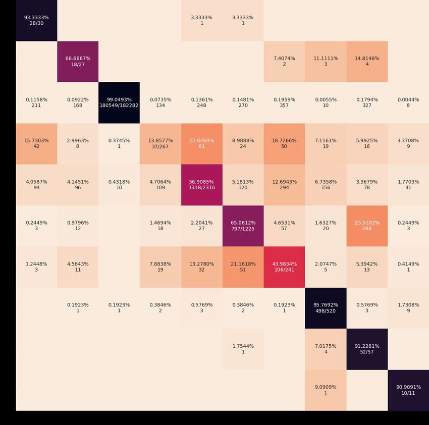
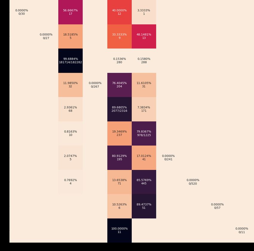
In figure 4.3 we can see the confusion matrix for MyNet trained using the standard
cross-entropy loss, we observe that all samples have been classified into the three
largest categories which is to be expected when training on an imbalanced dataset.
There is a notable amount of attack samples that have been classified as benign,
especially analysis have been mistakenly classified as safe. The model has achieved
high recall for classes it has classified with the lowest being exploits at 88.9%.
Figure 4.3: Confusion matrix for MyNet with Cross-entropy Loss
Looking at figure 4.4 we see that IoTNet has like MyNet only classified samples as
the largest classes, unlike MyNet fewer attack samples have been wrongly classified
as benign. Recall is similar or lower compared to MyNet with fuzzers dropping the
most from 91.60% down to 79.84%.
4.2.2 Re-sampling
Figure 4.5 shows the effect of using re-sampling with a weighted random sampler on
MyNet which has successfully classified samples of all categories. The best result is
for Worms with a recall of 100% as this is the smallest class it will have had the most4.2. Classification 21
Figure 4.4: Confusion matrix for IoTNet with Cross-entropy Loss22 Chapter 4. Results and Analysis
weight. DoS attacks were the most difficult to classify only being able to correctly
classify 37.08% which is more than 20% less then the second lowest attack type.
Figure 4.5: Confusion matrix for MyNet with Weighted Random Sampler
Observing figure 4.6 we can see some similarities for IoTNet to MyNet as both
struggled to correctly classify DoS samples this time only getting a recall of 13.86%.
Compared to MyNet with re-sampling the recall for which IoTNet was able to classify
shellcode was notably higher at 91.23%.
For both network when using re-sampling the number of samples miss classified
as benign were lower compared to when not using re-sampling. Overall the classifi-
cations were more spread out across all 10 categories indicating that the technique
is able to address some of the class imbalance present in the dataset.
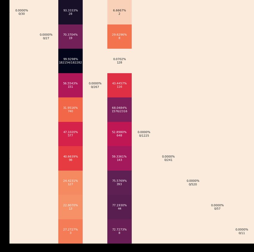
4.2.3 Cost sensitive learning
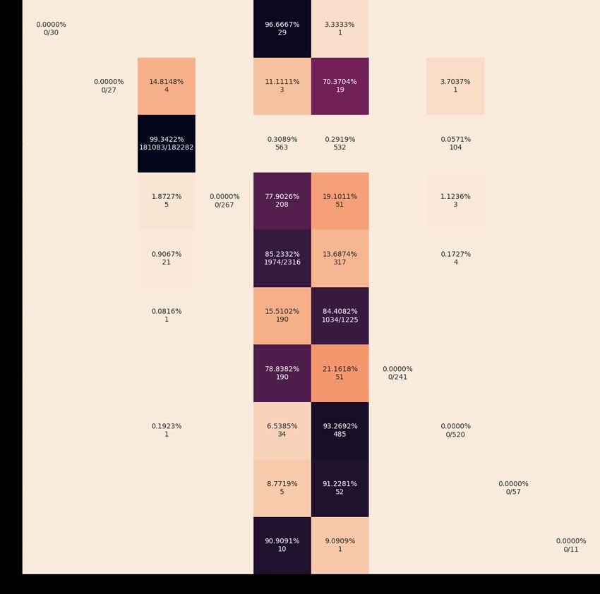
Weighted cross-entropy loss
Figure 4.7 illustrates how the use of a weighted cross-entropy loss affect the perfor-
mance of MyNet. We can see that the network was not able to detect any additional
classes, there is a slight decrease in the amount of attacks that got classified as benign
and there is also an increase of benign samples getting wrongly classified.4.2. Classification 23
Figure 4.6: Confusion matrix for IoTNet with Weighted Random Sampler24 Chapter 4. Results and Analysis
Figure 4.7: Confusion matrix for MyNet with Weighted Cross-Entropy Loss4.2. Classification 25
In figure 4.8 we see the results for IoTNet when using weighted cross-entropy
loss this shown an increase in the amount if classes used for classification with some
samples getting classified as reconnaissance, none of the samples that were classified
as reconnaissance were correctly classified. Like the case for MyNet we also see that
there were fewer false positives to the benign class and more false negatives for benign,
unlike MyNet there was an increase in recall for fuzzers and a decrease for exploits.
Figure 4.8: Confusion matrix for IoTNet with Weighted Cross-Entropy Loss
Class balanced loss
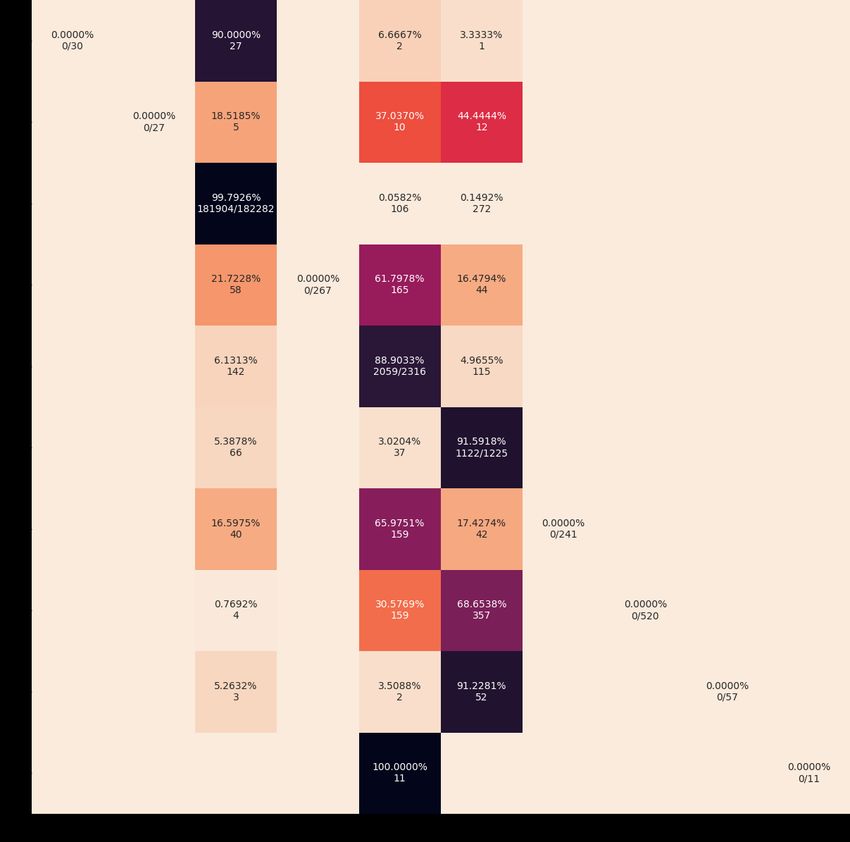
Observing figure 4.9 we can see that when using class balanced loss MyNet only
classified samples as the two largest categories with a large amount of false positives
to the benign class, this is worse than when not using any techniques to aid with
training on an imbalanced dataset as shown in figure 4.3.
Figure 4.10 shows the results of using class balanced loss with IoTNet that clas-
sified all samples as backdoor attacks which results in this model having the worst
performance by far.26 Chapter 4. Results and Analysis
Figure 4.9: Confusion matrix for MyNet with Class Balanced Loss4.2. Classification 27
Figure 4.10: Confusion matrix for IoTNet with Class Balanced Loss28 Chapter 4. Results and Analysis
4.2.4 Results summary
In table 4.3 the results of each class is presented for MyNet using re-sampling with a
weighted random sampler, with the difference to the results presented by Sarhan et.
al. shown in parenthesis [29]. MyNet has a higher recall in 6 out of 10 classes, the
highest lead is for analysis which has a recall rate of 0.93 which is 62.44% higher.
The F1 Score for all classes but one, backdoor is lower for MyNet, the class with
the best performance overall is benign. The overwhelmingly low precision is due to
the miss classifications being spread out across most classes which we can verify by
inspecting figure 4.5.
Class Accuracy Precision Recall (DR) F1 Score
Analysis 99.84% 0.088 0.93 (+62.44%) 0.16 (−0.01)
Backdoor 99.92% 0.11 0.67 (+26, 37%) 0.19 (+0.01)
Benign 97.51% 1.0 0.97 (−02.40%) 0.99 (−0.01)
DoS 99.72% 0.22 0.37 (+07.51%) 0.28 (−0.08)
Exploits 97.56% 0.29 0.67 (−13.27%) 0.41 (−0.43)
Fuzzers 99.66% 0.70 0.85 (+04.16%) 0.77 (−0.08)
Generic 99.76% 0.30 0.70 (−15.44%) 0.42 (−0.48)
Reconnaissance 99.87% 0.69 0.95 (+14.98%) 0.80 (−0.03)
Shellcode 99.88% 0.15 0.60 (−28.02%) 0.23 (−0.46)
Worms 99.97% 0.19 1.00 (+14.02%) 0.31 (−0.38)
Table 4.3: MyNet multi-class classification results
The result for IoTNet with re-sampling with a weighted random sampler is pre-
sented in table 4.4 per class using the same format as table 4.3. IoTNet has a larger
variance in precision and recall when compared to MyNet and had worse performance
in classifying generic as well as performing worse on fuzzers.
Class Accuracy Precision Recall (DR) F1 Score
Analysis 99.81% 0.073 0.93 (+62.44%) 0.14 (−0.03)
Backdoor 99.84% 0.057 0.67 (+26, 37%) 0.11 (−0.07)
Benign 99.07% 1.0 0.99 (−00, 80%) 1.0
DoS 99.73% 0.12 0.14 (−15, 71%) 0.13 (−0.23)
Exploits 99.27% 0.78 0.57 (−23, 50%) 0.66 (−0.18)
Fuzzers 99.52% 0.63 0.65 (−15, 51%) 0.64 (−0.21)
Generic 99.52% 0.12 0.44 (−41, 17%) 0.19 (−0.71)
Reconnaissance 99.87% 0.70 0.96 (+15, 75%) 0.81 (−0.02)
Shellcode 99.61% 0.067 0.91 (+03, 56%) 0.12 (−0.57)
Worms 99.96% 0.12 0.91 (+04, 93%) 0.22 (−0.47)
Table 4.4: IoTNet multi-class classification results
The worst categories to classify were analysis, backdoor, and DoS which falls in
line with the results presented by Sarhan et. al. we were able to get a higher recall4.2. Classification 29
in all aforementioned classes using MyNet with re-sampling. Our model fell behind
when it came to classifying exploits, generic, and shellcode [29].
4.2.5 Inference time
The inference time for the different models on the test set is presented in table 4.5.
At most we saw a variation in inference time of 4 seconds between MyNet using cost
sensitive learning and IoTNet using the weighted random sampler. No difference was
measured between the two methods for cost sensitive learning. The mean inference
time was 51s, as we measure inference of the whole test set we can extrapolate a
mean per sample inference time of 0.27 ms.
Model Time (s)
MyNet (CELoss/CBLoss) 50
MyNet Sampler 52
IoTNet (CELoss/CBLoss) 52
IoTNet Sampler 54
Table 4.5: Inference time of test setChapter 5
Discussion
The discussion of this thesis is split into five different sections, summarizing our
findings, the affect of our limitations, feasibility for a CNN based IDS on IoT, im-
provements that could be made, and answers to our research questions.
5.1 Summary of findings
From the results of the experiment we can see that it is possible to use a small CNN
to classify network attacks using the NF-UNSW-NB15-v2 dataset when using re-
sampling. Compared to the reference paper we were able to get a higher recall rate
for at least 50% of the classes for both MyNet and IoTNet, however we observed that
our models consistently had lower F1 scores which indicate that when our models
miss classify a sample they don’t have a tendency to a particular class this can be
seen in figure 4.5 and 4.6.
We were not able to see any high level of generalizability of our models, this tells
us that they are not suitable for detection of zero-day attacks, however by using a
hybrid technique to deal with the class imbalance and could improve generalizability.
5.2 Limitations
During the course of this thesis work we ran into some technical limitation that came
to limit the project more than expected at the start.
5.2.1 Parameter search
We made the decision to not employ a parameter search for all possible parameters,
instead we chose to only do smaller scale testing for what we believe to be the most
important hyperparameters, learning rate and batch size. Ideally we would have also
tweaked the number of groups and blocks to use in IoTNet and the dropout rate for
each dropout layer, the main reason for this decision is the time required to train a
model. The mean training time for IoTNet was just under 7 hours and a total of
100 hours were allocated to training the models, this included time for tweaking the
models and hyperparameters. Additionally 100 hours of training were allocated in
tandem with the implementation of the models this was however reserved to validate
that the models were functional and implemented correctly. It is possible that our
results could have been improved greatly by finding more suitable parameters.
3132 Chapter 5. Discussion 5.2.2 Dataset Initially when evaluating which dataset to use we were planning to use a larger dataset, however that dataset turned out to be too large and was even more imbal- anced then the one we ultimately chose. The imbalance and size prevented us from using only using a much smaller subset as the smallest class would only contain 1 or 2 samples resulting in an inability to learn that class. 5.2.3 Cross validation We would have liked to do 5-fold cross validation instead of a 3-way holdout method, but due to the imbalance in the dataset we needed it to be large or we would not get a good representation of each class. We believe this was the correct method to use for this situation as it reduces the training time needed. Due to this the generalization of our model is limited. 5.3 Feasibility of deep learning IDS on IoT 5.3.1 Classification The results from the experiment show that the quality of the classification for the models trained are far from good enough to be used as a intrusion detection system, all models that were trained had worse performance overall than the reference paper. By using the random sampler the results for some classes were good, however even then the precision of each class left a lot to be desired. It might be possible to get good results by using a hybrid model that employs both re-sampling and cost- sensitive learning, then additional weight can be added to the classes that have the worst results. 5.3.2 Training time The average training time for both tested networks mean that it is not possible to train on an IoT device, this was however never the plan instead the model should be trained externally in the cloud and then propagated to each IoT device which will handle inference of incoming packets. It might be possible to do small additional training batches on the IoT device where it only learn a select few samples of a new found attack. The training time of the deep learning model is important for an IDS so that it can quickly get updated in case there is a new attack that has been discovered, therefor the model should be able to train overnight preferably. IoTNet was also consistently slower at training than MyNet while getting worse classification results. 5.3.3 Inference time The mean time needed to classify the test set is 51 s which is 0.27 ms per sample. This speed is not functional for real time operation in the general case where it could result in an infinitely growing backlog if this was used as an IDS. However in the
You can also read