Processing Remote Sensing Data with Python - Faculty of Life and Environmental Sciences University of Iceland
←
→
Page content transcription
If your browser does not render page correctly, please read the page content below

Processing Remote Sensing Data with
              Python

              Ryan J. Dillon

    Faculty of Life and Environmental
                 Sciences
          University of Iceland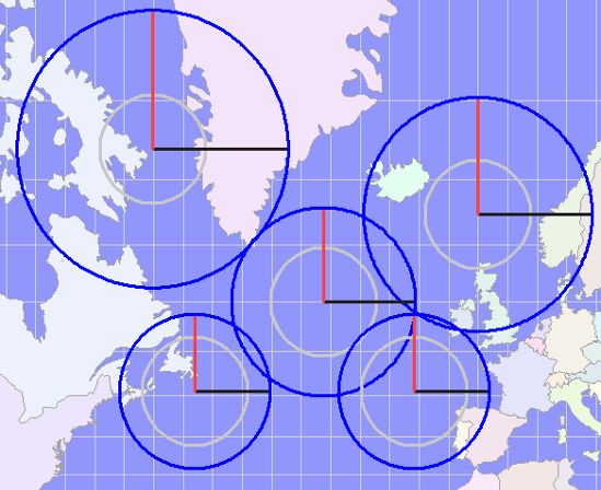
Processing Remote Sensing Data with
               Python

                        Ryan J. Dillon

        10 ECTS thesis submitted in partial fulfillment of a
Magister Scientiarum degree in Joint Nordic Masters Programme in
                  Marine Ecosystems and Climate

                Advisor / Faculty Representative

                     Guðrún Marteinsdóttir

           Faculty of Life and Environmental Sciences
           School of Engineering and Natural Sciences
                       University of Iceland
                      Reykjavik, June 2013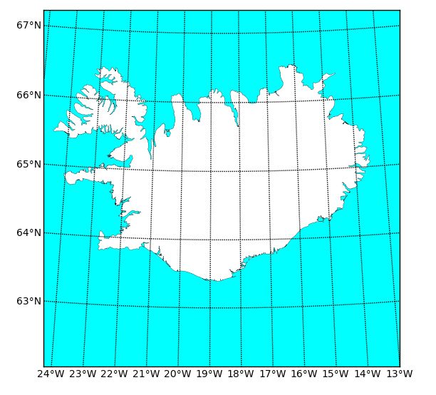
Processing Remote Sensing Data with Python
10 ECTS thesis submitted in partial fulfillment of a Magister Scientiarum degree in Joint
Nordic Masters Programme in Marine Ecosystems and Climate

Copyright © 2013 Ryan J. Dillon
All rights reserved

Faculty of Life and Environmental Sciences
School of Engineering and Natural Sciences
University of Iceland
Askja, Sturlugata 7
101, Reykjavik
Iceland

Telephone: 525 4600

Bibliographic information:
Dillon, Ryan J., 2013, Processing Remote Sensing Data with Python, Independent Study,
Faculty of Life and Environmental Sciences, University of Iceland
CONTENTS

1   Acknowledgements                                                                                                                 3

2   Introduction                                                                                                                     5
    2.1 Geosetup . . . . . . . . . . . . . . . . . . . . . . . . . . . . . . . . . . . . .                                           5
    2.2 Improving this Documentation . . . . . . . . . . . . . . . . . . . . . . . . . .                                             5

3   Brief Overview of Coordinate Systems and Map Projections                                                                         7
    3.1 Coordinate Systems . . . . . . . . . . . . . . . . . . . . . . . . . . . . . . .                                             7
    3.2 Earth’s Shape and Datums . . . . . . . . . . . . . . . . . . . . . . . . . . . .                                             8
    3.3 Map Projections . . . . . . . . . . . . . . . . . . . . . . . . . . . . . . . . .                                            8

4   Getting Started with Ocean Color and Bathymetric Data                                                                            11
    4.1 Data Formats . . . . . . . . . . . . . . . . . . . . . .                 .   .   .   .   .   .   .   .   .   .   .   .   .   11
    4.2 Data Properties . . . . . . . . . . . . . . . . . . . . .                .   .   .   .   .   .   .   .   .   .   .   .   .   12
    4.3 Focus Datasets . . . . . . . . . . . . . . . . . . . . .                 .   .   .   .   .   .   .   .   .   .   .   .   .   13
    4.4 Previewing Data . . . . . . . . . . . . . . . . . . . .                  .   .   .   .   .   .   .   .   .   .   .   .   .   18

5   Getting Started with Python                                                                                                      21
    5.1 Science and Python . . . . . . . . . . . .   .   .   .   .   .   .   .   .   .   .   .   .   .   .   .   .   .   .   .   .   21
    5.2 Troubleshooting . . . . . . . . . . . . .    .   .   .   .   .   .   .   .   .   .   .   .   .   .   .   .   .   .   .   .   21
    5.3 Important things to consider . . . . . . .   .   .   .   .   .   .   .   .   .   .   .   .   .   .   .   .   .   .   .   .   22
    5.4 Setting up your development environment      .   .   .   .   .   .   .   .   .   .   .   .   .   .   .   .   .   .   .   .   22

6   Importing netCDF and HDF Data with Python                                             25
    6.1 netCDF4 . . . . . . . . . . . . . . . . . . . . . . . . . . . . . . . . . . . . . 25

7   Working with Projections Using Python                                                    29
    7.1 pyproj . . . . . . . . . . . . . . . . . . . . . . . . . . . . . . . . . . . . . . . 29

8   Gridding and Resampling Data with Python                                               31
    8.1 Deciding what to do . . . . . . . . . . . . . . . . . . . . . . . . . . . . . . . 31
    8.2 Gridding . . . . . . . . . . . . . . . . . . . . . . . . . . . . . . . . . . . . . 31
    8.3 Re-sampling to Grid . . . . . . . . . . . . . . . . . . . . . . . . . . . . . . . 32

9   Plotting with Python                                                                 35
    9.1 Matplotlib and Basemap . . . . . . . . . . . . . . . . . . . . . . . . . . . . . 35

                                                                                                                                      i
10 Writing Geospatial Data to Files 39 10.1 Write file function . . . . . . . . . . . . . . . . . . . . . . . . . . . . . . . . 39 11 Geosetup - textdata 43 12 Geosetup - Pathfinder 45 13 Geosetup - CoRTAD 49 14 Geosetup - GlobColour 53 14.1 Importing Mapped L3m Data . . . . . . . . . . . . . . . . . . . . . . . . . . 53 14.2 Importing ISIN grid L3b Data . . . . . . . . . . . . . . . . . . . . . . . . . . 55 15 Geosetup - gebco 57 16 Geosetup - Main Program 61 17 Appendix: Temporal Coverage of Ocean Color Satellite Missions 67 17.1 Missions . . . . . . . . . . . . . . . . . . . . . . . . . . . . . . . . . . . . . 67 Bibliography 69 ii
CHAPTER

                                                                                      ONE

                                  ACKNOWLEDGEMENTS

First, I would like to thank the American Scandinavian Foundation in their support of my
work. I would also like to thank Guðrún Marteinsdóttir for her coordination and advising,
and Thorvaldur Gunlaugsson and Mette Mauritzen for their advising on my project for which
this coding is intended to support. Lastly, I am very appreciative toward Gisli Víkingsson and
Hafrannsóknastofnun for arranging a place for me to work.

                                                                                            3
Processing Remote Sensing Data with Python Documentation, Release 1 4 Chapter 1. Acknowledgements
CHAPTER

                                                                                           TWO

                                                          INTRODUCTION

With public access available for numerous satellite imaging products, modelling in atmospheric
and oceanographic applications has become increasingly more prevalent.
Though there are numerous tools available for geospatial development, their use is more com-
monly applied towards mapping applications. With this being the case, there are a number of
valuable texts for using these tools in such mapping applications [11] [1]; though, documenta-
tion for processing of remote sensing datasets is limited to brief contributions on personal blogs
or manual pages and tutorials specific to one library or dataset. Python programming methods
for performing such tasks will be focused on here, collecting various code and information
from these text, blogs, etc. and presenting original code that may be employed in scripts to
perform commonly required tasks in processing remote sensing data.
For a general place to get started with geospatial work with Python, Erik Westra’s “Python
Geospatial Development” is an excellent resource, and it will provide an excellent overview of
geospatial work with python before looking at specific remote sensing datasets.

2.1 Geosetup

The tools presented here are collected into a Python program repository(currently under devel-
opment) that will produce standardized gridded satellite data files that may be used as input for
various models. This repository is publicy available on the collaborative coding site GitHub.
Link to repository on GitHub: https://github.com/ryanjdillon/geosetup
Or, you may download the code as a zip-archive.
If you are interested in collaborating on this effort, please feel encouraged to fork the repository
on GitHub and offer your contributions.

2.2 Improving this Documentation

There are many improvements that can always be made in either the code shown here, or the
explanation of a particular approach to something. If you find something broken, or stuck with
an inadequate explanation, feel free to contact me so that I might correct it.

                                                                                                  5
Processing Remote Sensing Data with Python Documentation, Release 1 Thanks, Ryan ryanjamesdillon@gmail.com 6 Chapter 2. Introduction
CHAPTER

                                                                                   THREE

     BRIEF OVERVIEW OF COORDINATE
     SYSTEMS AND MAP PROJECTIONS

Before working with georeferenced datasets, it is important to understand how things can be
referenced geographically.
Positions on earth’s surface can be represented using different systems, the most accurate of
these being geodetic positions determined by coordinates from a particular geographic coordi-
nate system, or geodetic system.
In addition to coordinate systems, the assumed shape of the earth will affect how coordinate
positions are translated to earth’s surface. Geodetic Datums are mathematical definitions of
for the shape of the earth, which in turn defines a geodetic system.

3.1 Coordinate Systems

Coordinate systems are categorized into two groups, both of which being commonly used in
representing remote sensing data:
    • unprojected coordinate systems these are 3-dimensional coordinate systems, such as
      latitude and longitude (referred to as Geographic Coordinate System in common GIS
      software)
    • projected coordinate systems these are 2-dimensional, there are many all of which hav-
      ing an advantage over another for a particular use.
Either system may be used depending on the data format (e.g. netCDF HDF containing arrays
of unprojected data vs. GeoTIFF images containing projected data). When working with
multiple datasets, or doing some processing of a dataset, you may need to change between
different coordinate systems.
Most often data will coincide with a latitude and longitude (i.e. unprojected). If it is desired
to interpolate or re-sample this data, transforming the data to a projected system allows for
simpler and a greater variety of methods to be used.

                                                                                              7
Processing Remote Sensing Data with Python Documentation, Release 1 3.2 Earth’s Shape and Datums It is often easiest to make the assumption that the earth is a perfect sphere when working with spherical coordinates. However, the earth’s shape is in fact an oblate ellipsoid, with its polar radius being approximately 21 km less then the equatorial radius [9]. This shape has been calculated using different systems for both the entire globe and for regional areas, known as datums. The most widely used datum for Geographic Information Systems is the World Geodetic Sys- tem (WGS84), which is used by most Global Positions System (GPS) devices by default. It is important to know which datum was used to record positions of data, as there can be sizable differences between actual physical position of points with the same coordinates, depending on the datum. 3.3 Map Projections In order to better visualise the earths surface and simplify working with certain geographic in- formation, 2-dimensional representations can be calculated using various mathematical trans- formations. Depending on the size of the area of interest (i.e. a small coastal area vs. an entire ocean) different projections will provide the greatest accuracy when interpolation of data is necessary. 3.3.1 Mercator The Mercator Projection is commonly used for general mapping applications where visualiza- tion is a priority over accuracy of size and shape near the poles. Variations of it are used for mapping applications, such as is used for Google Maps [15]. Though useful for many mapping applications, this projection should be avoided when inter- polation of data is necessary due to increasing distortion error near the poles. 3.3.2 UTM The Universal Transverse Mercator (UTM) projection is a variation of the Mercator projection, which uses a collection of different projections of 60 zones on the earths surface to allow accurate positioning and minimal distortion on a 2-dimensional projection [8]. Though this system provides a way of accurate approach to a Mercator, it becomes difficult to work with when the area of interest spans multiple zones. 8 Chapter 3. Brief Overview of Coordinate Systems and Map Projections
Processing Remote Sensing Data with Python Documentation, Release 1

Figure 3.1: Mercator projection with Tissot circles showing increased distortion near the poles
[5].

Figure 3.2: Universal Transverse Mercator (UTM) projection displaying the different zones [8]

3.3. Map Projections                                                                         9
Processing Remote Sensing Data with Python Documentation, Release 1

3.3.3 Albers Equal-Area

The Albers equal-area conic projection is a projection that is useful where area needs to be pre-
served for large geographical areas. When working with data, as is needed when interpolating
data over such an area.

            Figure 3.3: Albers Equal-Area Conic projection with Tissot circles [5].

10        Chapter 3. Brief Overview of Coordinate Systems and Map Projections
CHAPTER
FOUR
GETTING STARTED WITH OCEAN
COLOR AND BATHYMETRIC DATA
The datasets that will be focussed on are those containing parameters that are most generally
applicable to marine ecosystem modeling: sea surface temperature, chlorophyll a, and bottom
depth. The concepts and methods used for these may be extrapolated to other datasets, and
should provide a good framework for processing such data.
4.1 Data Formats
4.1.1 netCDF HDF
The most common formats used for oceanographic and atmospheric datasets are Unidata’s
Network Common Data Form (netCDF) and HDF Group’s Hierarchical Data Format (HDF)
[18] [20].
Both of these formats have gone through multiple revisions, with different functionality and
backwards compatibility being available between versions, with the latest versions being in
most common use, netCDF-4 and HDF5 respectively.
As the name describes, HDF is hierarchical in its internal organization, which has many ad-
vantages particularly advanced organization of data and efficient storage and access to large
amounts of data. HDF5 is the most current and widely used HDF format with many tools and
libraries for accessing and creating datasets in this format.
4.1.2 GeoTIFF
Another common format for geospatial data is in the form of raster data, or data that is repre-
sented by grid cells particularly in the form of an image, such as GeoTIFF files.
The GeoTIFF format is a standardized file format, which is a modification of the Tagged Image
File Format (TIFF) specially suited for storing datasets referenced in a projected coordinate
system. Each data value will correspond to a grid cell (i.e. pixel) of the image, which is saved
as a tag as metadata together with the image data [10]. The images pixel corresponds to an area
enclosed by geographic boundaries defined by the projection used to create that GeoTIFF.
11Processing Remote Sensing Data with Python Documentation, Release 1
4.1.3 Arc/Info ASCII Grid and Binary Grid
Due to the popularity of ESRI’s ArcGIS software, another format commonly seen is Arc/Info
ASCII grid format and binary grid format. Developed by ESRI for their ArcGIS software, both
formats store data in a similar way to GeoTIFF in that they relate a set of data values to grid
cell areas, defined by some geographic bounds.
The binary format is a proprietary format that was developed to add functionality and prevent
unlicensed use of data produced by their software.
The Arc/Info ASCII Grid is a simple ASCII text file format that is still found in used by some
due to its simple non-proprietary format. The ASCII format includes a series of header rows
defining the rows and columns in the grid, position of the center and corners, cell size, fill value
for missing data, and then space-delimited values. As described by the Oak Ridge National
Laboratory site [17]:
{NODATA_VALUE xxx}
row 1
row 2
.
.
.
row n
Note: There are many other raster image formats besides GeoTIFF and Arc/Info grid formats
that geospatial data can be stored in. The GDAL libraries are capable of working with most of
them, a list of which can be found here [19].
4.2 Data Properties
4.2.1 Data Levels
In some instances one may want to perform their own processing of raw satellite data, but for
our purposes here, we will just be concerned with working with data that has already been
evaluated for quality and averaged into regular time allotments.
It is useful to be familiar with the different types of ‘levels’ that are available, so that you may
select the proper data to begin working with [16]:
12 Chapter 4. Getting Started with Ocean Color and Bathymetric DataProcessing Remote Sensing Data with Python Documentation, Release 1
Level Code Description
Level 0 L0 Raw instrument data
Level L1A Reconstructed raw instrument data
1A
Level L1B Products containing geolocated and calibrated spectral radiance and solar
1B irradiance data
Level 2 L2 Products derived from the L1B product. One file per orbit
Level 3 L3 Averaged global gridded products, screened for bad data points
Level 4 L4 Model output; derived variables
With this information, we can see that we are most interested in the Level 3 (L3) data sets.
4.3 Focus Datasets
The datasets that will be covered are those for which methods have been written in Geosetup.
For data that is accessible via an FTP server, any standard FTP-client can be used for down-
loading the data (e.g. Filezilla) [6]. On UNIX-like systems this can more easily be done by
using the wget command.
4.3.1 Pathfinder
Pathfinder is a merged data product from the National Oceanographic Data Center (NODC)
[23], an office of the National Oceanic and Atmospheric Association (NOAA).
Summary
• Data Format: HDF5
• Date Range: 1981-2011 (gap from 1994-05-27 to 1995-07-01)
• Timestamps: in days from reference time ‘1981-01-01 00:00:00’
• Data quality control: variable containing quality flags for data points
Variables in Dataset
Downloading
Pathfinder data is available to download via HTTP, FTP, THREDDS (supporting OPeNDAP),
and rendered images/KML [23].
Example for downloading all Pathfinder v5.2 data for 2007:
wget -r -np -nH ftp://ftp.nodc.noaa.gov/pub/data.nodc/pathfinder/Version5.2/2007
4.3. Focus Datasets 13Processing Remote Sensing Data with Python Documentation, Release 1
Figure 4.1: Panoply output showing datasets included in Pathfinder v5.2 datafile
4.3.2 CoRTAD
CoRTAD is a reprocessed weekly average dataset of the Pathfinder data, developed by National
Oceanographic Data Center (NODC) [22] for modelling and management of coral reef systems.
Summary
• Data Format: HDF5
• Date Range: 1981-2011 (gap from 1994-05-27 to 1995-07-01)
• Timestamps: in days from reference time ‘1981-01-01 00:00:00’
• Data quality control: Two separate data variables are included, including one where gaps
due to clouds, etc. have been interpolated. Also included is an array of all bad data, and
a variety of variables providing statistical evaluation of all data.
Variables in Dataset
Downloading
On UNIX-like systems, you may use a file with a list of the URL’s for all files you would like
to download. Then you can use the wget command with the -i option to download all files in
the list.
Example cortad_wget-list.txt
ftp://ftp.nodc.noaa.gov/pub/data.nodc/cortad/Version4/cortadv4_row01_col05.nc
ftp://ftp.nodc.noaa.gov/pub/data.nodc/cortad/Version4/cortadv4_row00_col09.nc
ftp://ftp.nodc.noaa.gov/pub/data.nodc/cortad/Version4/cortadv4_row01_col09.nc
Example wget command:
14 Chapter 4. Getting Started with Ocean Color and Bathymetric DataProcessing Remote Sensing Data with Python Documentation, Release 1
Figure 4.2: Panoply output showing datasets included in CoRTAD datafile
4.3. Focus Datasets 15Processing Remote Sensing Data with Python Documentation, Release 1
wget -i cortad_wget-list.txt
4.3.3 GlobColour Chlorophyll-a Data
The European Space Agency (ESA) produces a merged chlorophyll dataset that combines data
acquired from the SeaWiFS (NASA), MODIS (NASA), and MERIS (ESA) satellite imaging
missions.
A very extensive explanation of the data and its derivation is covered in the GlobColour Product
User Guide. You may download it from their website here:
http://www.globcolour.info/CDR_Docs/GlobCOLOUR_PUG.pdf
This merged data product is ideal for applications where your sampling period may extend be-
yond that covered by any one when your sampling period extends across the acquisition periods
of each of the different missions offering imagery in a spectral range from which chlorophyll
values may be processed from.
Note: See Temporal ranges of ocean color satellite missions for coverage of different datasets.
Different merging methods have been used, including:
• simple averaging
• weighted averaging
• GSM model
Grid Formats
Integerized Sinusoidal (ISIN) L3b Product
• Angular resolution: 1/24◦ (approx. 4.63km spatial resolution)
• Uses rows and cols arrays to specify the latitudinal and longitudinal index of the
bins, stored in the product (i.e. mean chlorophyll values in CHL1_mean)
Plate-Carré projection (Mapped) L3m Product
• Angular resolution: 0.25◦ and 1.0◦
• latitude and longitude specifying the center of each cell
Note: The mapped (L3m) product is an easier format to work, as it uses standard coordinate
and value organization, but you will need to use the ISIN grid (L3b) product if you require th
~4.63 km resolution.
16 Chapter 4. Getting Started with Ocean Color and Bathymetric DataProcessing Remote Sensing Data with Python Documentation, Release 1
Summary
• Data Format: netCDF-3
• Date Range: 1981-2011 (gap from 1994-05-27 to 1995-07-01)
• Timestamps: in hours from reference time ‘1981-01-01 00:00:00’
• Data quality control: variable containing quality flags for data points
Variables in Dataset
Figure 4.3: Panoply output showing datasets included in Globcolour datafile
Downloading
Data can be downloaded for specific time periods and geographic extents through their gui
download interface on the web:
http://hermes.acri.fr/GlobColour/index.php
ESA’s also maintains an ftp-server from which you may download GlobColour data in batch,
for a large number of files.
Example for downloading GSM averaged 1-Day Chlorphyll-a between 1997-2012:
wget -r -l10 -t10 -A "*.gz" -w3 -Q1000m \
ftp://globcolour_data:fgh678@ftp.acri.fr/GLOB_4KM/RAN/CHL1/MERGED/GSM/{1997,1998
4.3.4 GEBCO Bathymetric Data
The General Bathymetric Chart of the Oceans is a compilation of a ship depth soundings and
satellite gravity data and images. Using quality-controlled data to begin with, values between
sounded depths have been interpolated with gravity data obtained by satellites [13].
Source Identifier (SID) Grid describes which measurements are from soundings or predictions.
Summary
• Data Format: netCDF-3
• Angular resolution: 30sec and 1◦ grids
4.3. Focus Datasets 17Processing Remote Sensing Data with Python Documentation, Release 1
– (0,0) position at northwest corner of file
– Grid pixels are center-registered
• Data organization: Single data file for whole globe
– 21,600 rows x 43,200 columns = 933,120,000 data points
• Units: depth in meters. Bathymetric depths are negative and topographic positive
• Date Range: Dates of soundings vary. Most recent 2010
• Data quality control: separate file with SID grid of data sources and quality.
Variables in Dataset
Figure 4.4: Panoply output showing datasets included in GEBCO datafile
Downloading
Before downloading the GEBCO data, you mush register at their website first. Follow link to
register
After registration, you can access the data here. You will have the option of downloading either
the gebco_08.nc file for the 30sec gridded data or the gridone.nc file for the 1◦ .
You may also download the SID grid which contains flags corresponding to each data point as
to whether it is a sounding or interpolated, and the quality of each.
4.4 Previewing Data
Various applications are available for viewing netCDF and HDF formatted data, but not all are
capable of opening versions of both formats such as both HDF5 and netCDF3.
When writing code to work with such data sets, it is often necessary to know the names and
dimensions of variables withing the datafile, which a viewing application makes particularly
easy.
18 Chapter 4. Getting Started with Ocean Color and Bathymetric DataProcessing Remote Sensing Data with Python Documentation, Release 1
4.4.1 Panoply
Panoply is a viewer application developed by NASA that allows a number of useful tools for
exploring data in netCDF, HDF, and GRIB formats.
Note: Panoply is dependent on the Java runtime environment, which must be installed before
installing. Download Java
Panoply Download Link:
http://www.giss.nasa.gov/tools/panoply/
Some Neat Features
• Slice and plot data sets, combining them, and save to image files
• Connect to OPeNDAP and THREDDS data servers to explore data remotely
• Create animations from collection of images
4.4.2 VISAT Beam
The ESA had commissioned the development BEAM of an open-source set of tools for viewing,
analyzing and processing are large number of different satellite data products [14]. In addition
they have developed the GUI desktop application VISAT for using these tools
Dowloand LSAT/BEAM
4.4.3 Quantum GIS
Quantum GIS is an open source GIS application that is available for all major operating systems
and has features similar to those found in much more costly GIS applications.
It is an excellent resource when viewing images created by your scripts, and has the ability to
be extended with PyQGIS once you become familiar with Python and working with geospatial
data.
Download Quantum GIS
4.4. Previewing Data 19Processing Remote Sensing Data with Python Documentation, Release 1 20 Chapter 4. Getting Started with Ocean Color and Bathymetric Data
CHAPTER

                                                                                       FIVE

        GETTING STARTED WITH PYTHON

Quickstart
Skip to installation and package guide

If you have previous experience programming, learning Python is a fairly intuitive process with
syntax that is easily read and remembered compared to other lower level languages like C/C++.
A good place to start is with Google’s free online python course:
      https://developers.google.com/edu/python/

5.1 Science and Python

Along with gaining a general familiarity in Python, you will want to become familiar with the
use of NumPy, as this module is used extensively for working with large datasets in an efficient
manner. In addition the netCDF4 module that is used here for opening netCDF and HDF
datasets by default creates masked NumPy array when importing these datasets.
The SciPy team has a great NumPy tutorial to get started with:
      http://www.scipy.org/Tentative_NumPy_Tutorial
Though not really covered in this article, the Python Data Analysis Library (Pandas) has in-
credible tools for data processing and working with statistical analysis and modelling. In com-
bination together, Python, NumPy/SciPy, and Pandas offers a powerful data processing ability,
rivalling R and Matlab with functionality that does not exist in either .

5.2 Troubleshooting

iPython is an excellent tool for working interactively with python, allowing you to test code,
play with concepts you are exploring, and store various information in a workspace similar to
R and Matlab work flows [2] [21].
When hitting stumbling blocks or just trying to improve your code, StackOverflow is a fantastic
resource for receiving support and finding existing solutions to your problems.

                                                                                             21
Processing Remote Sensing Data with Python Documentation, Release 1
5.3 Important things to consider
• Backup! In more than two places preferably. It takes a long time to code, and you don’t
want to start over if something happens.
• Along with general backups, using a version control system such as Git, Subversion,
or Mercurial. Doing so allows you to easily revert to previous versions of your code,
collaborate with others, track problems, develop in stages, and more.
• Stick to the conventions: coding like everybody else (e.g. naming, spacing, commenting,
etc.) makes things easier for you and for others to work with your code.
5.4 Setting up your development environment
The code here was developed using Python version 2.7; however it should be compatible with
versions greater the 2.6.
5.4.1 Installing Python
Python can be downloaded from Python.org as source, as well as binary installers for Windows
and Mac OSX.
Most distributions of Linux come with Python pre-installed. To see what version of python you
are running, run the following from the command line python -V.
5.4.2 Additional Python Packages you will need
In order to properly run the code presented here, you will need to also install a number of other
libraries/packages that are used.
It will just be assumed that if you are using another distribution of Linux/UNIX than Ubuntu,
that you will be familiar enough to hunt down the packages/source and install them.
• gdal
– Ubuntu (linux): https://launchpad.net/~ubuntugis/+archive/ppa/
– Windows: Install OSGeo (with GDAL): http://trac.osgeo.org/osgeo4w/wiki
– Mac OSX: Pre-compiled binaries http://www.kyngchaos.com/software/frameworks#gdal_com
• pyroj
– Ubuntu (linux): http://packages.ubuntu.com/search?keywords=python-pyproj
– Windows: http://code.google.com/p/pyproj/downloads/list
– Mac OSX (Unverified): http://mac.softpedia.com/get/Math-
Scientific/pyproj.shtml
22 Chapter 5. Getting Started with PythonProcessing Remote Sensing Data with Python Documentation, Release 1
• numpy
– Ubuntu (linux): from command line sudo apt-get install
python-numpy
– Windows: http://sourceforge.net/projects/numpy/files/NumPy/
– Mac OSX: http://www.scipy.org/Installing_SciPy/Mac_OS_X
• scipy
– Ubuntu (linux): from command line sudo apt-get install
python-scipy
– Windows: http://www.scipy.org/Installing_SciPy/Windows
– Mac OSX: http://www.scipy.org/Installing_SciPy/Mac_OS_X
• matplotlib
– All operating systems: http://matplotlib.org/faq/installing_faq.html#installation
• matplotlib.basemap
– To be installed as above, just note that it must be installed in addition to mat-
plotlib
5.4.3 Getting Geosetup
In order to collaborate to the code, it is preferable that you obtain the Geosetup code by
forking the repository from GitHub.
If you’re new to Git, a comprehensive instructional book is available here [3]:
If you prefer you may download the code as a ZIP archive, or access it from the repository page
on GitHub.
5.4. Setting up your development environment 23Processing Remote Sensing Data with Python Documentation, Release 1 24 Chapter 5. Getting Started with Python
CHAPTER

                                                                                              SIX

       IMPORTING NETCDF AND HDF DATA
                        WITH PYTHON

    The first thing you’ll need to do to work with these datasets is to import it to

    6.1 netCDF4

    netCDF4 is a python package that utilizes NumPy to read and write files in netCDF and HDF
    formats [12]. It contains methods that allow the opening and writing of netCDF4, netCDF3
    and HDF5 files.
    Before importing the data, you’ll want to find the name of the dataset variable that you want to
    import. You can determine this by first opening the file with Panoply and checking the name of
    the variable. Examples for the different variables available from this paper’s focus datasets is
    found in the summaries sections of Focus Datasets.
    Example showing the data import using netCDF4:
    import numpy as np
    import netCDF4 as Dataset

    filepath = /path/to/file.nc
    # Read in dataset (using ’r’ switch, ’w’ for write)
    dataset = Dataset(filepath,’r’)
    # Copy data to variables, ’[:]’ also copies missing values mask
    lons = dataset.variables["lon"][:]
    lats = dataset.variables["lat"][:]
    sst = dataset.variables["sea_surface_temperature][:]
    dadtaset.close()

    When data is copied to a variable in Python, it places it all into the systems temporary memory,
    which means there is a limit as to how much data can be loaded. With certain datasets, the
    dataset variables may be large enough to exceed the system memory.
    Typically these datasets cover much larger geographic areas than are interested in (i.e. the
    whole earth), so it is possible to load only the data for the area of interest.
1        def getnetcdfdata(data_dir, nc_var_name, min_lon, max_lon, min_lat, max_lat, data_time_start, data_time_e
2        ’’’Extracts subset of data from netCDF file
3
4        based on lat/lon bounds and dates in the iso format ’2012-01-31’ ’’’
5
6        # Create list of data files to process given date-range

                                                                                                 25
Processing Remote Sensing Data with Python Documentation, Release 1
7 file_list = np.asarray(os.listdir(data_dir))
8 file_dates = np.asarray([datetime.datetime.strptime(re.split(’-’, filename)[0], ’%Y%m%d%H%M%S’) for filen
9 data_files = np.sort(file_list[(file_dates >= data_time_start)&(file_dates math.floor(min_lon))&(lons < math.ceil(max_lon)))[0]
18 lats_idx = np.where((lats > math.floor(min_lat))&(lats < math.ceil(max_lat)))[0]
19 x_min = lons_idx.min()
20 x_max = lons_idx.max()
21 y_min = lats_idx.min()
22 y_max = lats_idx.max()
23
24 # Create arrays for performing averaging of files
25 vals_sum = np.zeros((y_max-y_min + 1, x_max-x_min + 1))
26 vals_sum = ma.masked_where(vals_sum < 0 , vals_sum)
27 mask_sum = np.empty((y_max-y_min + 1, x_max-x_min + 1))
28 dataset.close()
29
30 # Get average of chlorophyl values from date range
31 file_count = 0
32 for data_file in data_files:
33 current_file = os.path.join(data_dir,data_file)
34 dataset = Dataset(current_file,’r’) # by default numpy masked array
35 vals = np.copy(dataset.variables[nc_var_name][0 ,y_min:y_max + 1, x_min:x_max + 1])
36 #vals = ma.masked_where(vals < 0, vals)
37 #ma.set_fill_value(vals, -999)
38 vals = vals.clip(0)
39 vals_sum += vals
40 file_count += 1
41 dataset.close()
42 vals_mean = vals_sum/file_count #TODO simple average
43
44 # Mesh Lat/Lon the unravel to return lists
45 lons_mesh, lats_mesh = np.meshgrid(lons[lons_idx],lats[lats_idx])
46 lons = np.ravel(lons_mesh)
47 lats = np.ravel(lats_mesh)
48 vals_mean = np.ravel(vals_mean)
49
50 return lons, lats, vals_mean
Another option for avoiding this problem is by loading the data in chunks, using sparse arrays,
or python libraries that allow loading the data onto the system hard drive, such as PyTables or
h5py.
6.1.1 OPeNDAP & THREDDS
Rather than opening the data from files on your local machine, it is possible to open them
remotely. Rather than creating the dataset from a local data file path, you simply reference the
path to a file on a remote OPeNDAP or THREDDS server.
To create a dataset for data located at http://data.nodc.noaa.gov/opendap/pathfinder/Vers
you would simply do the following:
1 import numpy as np
2 import netCDF4 as Dataset
3
4 filepath = ’http://data.nodc.noaa.gov/opendap/pathfinder/Version5.2/1981/19811101025755-NODC-L3C_GHRSST-S
5 # Read in dataset (using ’r’ switch, ’w’ for write)
6 dataset = Dataset(filepath,’r’)
26 Chapter 6. Importing netCDF and HDF Data with PythonProcessing Remote Sensing Data with Python Documentation, Release 1 For further information on these protocols, thorough explanations are presented on their web- sites. OPeNDAP THREDDS 6.1. netCDF4 27
Processing Remote Sensing Data with Python Documentation, Release 1

28                   Chapter 6. Importing netCDF and HDF Data with Python
CHAPTER

                                                                                   SEVEN

               WORKING WITH PROJECTIONS
                           USING PYTHON

7.1 pyproj

pyproj is a python interface to the PROJ.4 library which offers methods for working between
geographic coordinates (e.g. latitude and longitude) and Cartesian coordinates (i.e. two dimen-
sional projected coordinates - x,y) [4].

7.1.1 Defining variables from pyproj class instances

It is possible to extract information from pyproj ellipsoid and projection class instances if
needed for other calculations.
As an example, let us first define an ellipsoid using the WGS84 datum:
g = pyproj.Geod(ellps=’WGS84’)

If we were to want to use the radius of the earth of this ellipsoid for another calculation, we
could extract the value to a variable from the pyproj ellipsoid class instance we defined above.
To find the value, you can use the dir() function to find the names that are defined by a mod-
ule. We can see by the following that the first variable listed (i.e. not an __attribute__) is
a:
dir(g)
>>> dir(g)
[’__class__’, ’__delattr__’, ’__dict__’, ’__doc__’, ’__format__’, ’__getattribut

You may access these by using either getattr function (if you have the property name as a
string or would like to access it dynamically) or more simply when we know the name of the
property by just using the dot notation:
>>> getattr(g,’a’) # getattr function
6378137.0

>>> g.a # dot notation
6378137.0

                                                                                             29
Processing Remote Sensing Data with Python Documentation, Release 1
If we hadn’t already known that a was the value we were looking for, we could have just used
the dot notation as above to have output the various values that were available in this object.
To make things easier to read later, you could do the following:
earth_equa_radius = g.a # earth’s radius at the equator in meters
earth_pole_radius = g.b # earth’s radius through poles in meters
7.1.2 Defining a projection
Example of defining a projection using the EPSG code:
import pyproj
# LatLon with WGS84 datum used by GPS units and Google Earth
wgs84 = pyproj.Proj(init=’EPSG:4326’)
# Lambert Conformal Conical (LCC)
lcc = pyproj.Proj(init=’EPSG:3034’)
Not all projections are available by using the ESPG reference code, but it is possible to define
your own projection using pyproj and gdal in python.
Spatialreference is a great resource for finding the details for the projection you’d like to create
(assuming it’s just not in the library; though, feel free to define a completely custom projection).
Example of defining the Albers projection:
# Albers Equal Area Conic (aea)
nplaea1 = pyproj.Proj("+proj=laea +lat_0=90 +lon_0=-40 +x_0=0 +y_0=0 \
+ellps=WGS84 +datum=WGS84 +units=m +no_defs")
30 Chapter 7. Working with Projections Using PythonCHAPTER
EIGHT
GRIDDING AND RESAMPLING DATA
WITH PYTHON
When using remote sensing data for model applications, you will want to somehow standardize
everything to a uniform grid. Your data may be scattered, and the satellite data be arranged at
different resolutions and grids (and perhaps using different projections).
8.1 Deciding what to do
8.1.1 Choosing an Interpolation Method
Depending on the type of data that you will be re-sampling to a grid, different interpolation
methods may be better suited to your data.
It is possible to interpolate data referenced by an unprojected coordinate system; though, due
to more complicated calculations involved and potential differences in the datasets, it may be
easiest to first project the data. The type of projection that is chosen to project the data to before
interpolating it using a 2-dimensional interpolation method depends upon the exent of the study
area and latitudes at which the data exist.
8.1.2 Choosing a Cartesian Projection
In general, you should attempt to choose a projection that does not distort the area over which
the area exists, introducing error in you interpolation product, such as using the Albers Equal
Area projection for a large area extending into northern latitudes (e.g. the North Atlantic ocean)
(see Map Projections).
8.2 Gridding
Before interpolating the data to a new grid, you will want to create that grid, defined by latitude
and longitude coordinates.
31Processing Remote Sensing Data with Python Documentation, Release 1
8.2.1 Creating a grid
Create Grid:
import numpy as np
def creategrid(min_lon, max_lon, min_lat, max_lat, cell_size_deg, mesh=False):
’’’Output grid within geobounds and specifice cell size
cell_size_deg should be in decimal degrees’’’
min_lon = math.floor(min_lon)
max_lon = math.ceil(max_lon)
min_lat = math.floor(min_lat)
max_lat = math.ceil(max_lat)
lon_num = (max_lon - min_lon)/cell_size_deg
lat_num = (max_lat - min_lat)/cell_size_deg
grid_lons = np.zeros(lon_num) # fill with lon_min
grid_lats = np.zeros(lat_num) # fill with lon_max
grid_lons = grid_lons + (np.assary(range(lon_num))*cell_size_deg)
grid_lats = grid_lats + (np.assary(range(lat_num))*cell_size_deg)
grid_lons, grid_lats = np.meshgrid(grid_lons, grid_lats)
grid_lons = np.ravel(grid_lons)
grid_lats = np.ravel(grid_lats)
#if mesh = True:
# grid_lons = grid_lons
# grid_lats = grid_lats
return grid_lons, grid_lats
8.3 Re-sampling to Grid
8.3.1 Without Projecting
It is possible to take the geographic coordinates and interpolate them over a spherical surface,
rather than first projecting the data, and then performing the interpolation on a 2-dimensional
surface. This can be done using scipy.interpolator.RectSphereBivariateSpline‘s smoothing
spline approximation:
import numpy as np
from scipy.interpolate import RectSphereBivariateSpline
def geointerp(lats,lons,data,grid_size_deg, mesh=False):
’’’We want to interpolate it to a global x-degree grid’’’
deg2rad = np.pi/180.
new_lats = np.linspace(grid_size_deg, 180, 180/grid_size_deg)
new_lons = np.linspace(grid_size_deg, 360, 360/grid_size_deg)
new_lats_mesh, new_lons_mesh = np.meshgrid(new_lats*deg2rad, new_lons*deg2rad)
’’’We need to set up the interpolator object’’’
lut = RectSphereBivariateSpline(lats*deg2rad, lons*deg2rad, data)
’’’Finally we interpolate the data. The RectSphereBivariateSpline
object only takes 1-D arrays as input, therefore we need to do some reshaping.’’’
new_lats = new_lats_mesh.ravel()
new_lons = new_lons_mesh.ravel()
data_interp = lut.ev(new_lats,new_lons)
if mesh == True:
32 Chapter 8. Gridding and Resampling Data with PythonProcessing Remote Sensing Data with Python Documentation, Release 1
data_interp = data_interp.reshape((360/grid_size_deg,
180/grid_size_deg)).T
return new_lats/deg2rad, new_lons/deg2rad, data_interp
Limitations:
• This method is restricted to using the smoothing spline approximation, which may not
be the best method for your data
• It assumes a spherical earth, where using the WGS84 datum would more accurately rep-
resent the data on the ellipsoid earth.
8.3. Re-sampling to Grid 33Processing Remote Sensing Data with Python Documentation, Release 1 34 Chapter 8. Gridding and Resampling Data with Python
CHAPTER

                                                                                           NINE

                                   PLOTTING WITH PYTHON

     9.1 Matplotlib and Basemap

     Matplotlib is a versatile plotting library that was developed by John Hunter that may be used
     for everything from basic scatter plots to cartographic plots, along with remote sensing data.
     Matplotlib basemap is an additional library to matplotlib which may be used for plotting
     maps and 2-dimensional data on them. It performs similar functionality to pyproj (and uses
     the same PROJ.4 libraries) to transform data to 2-dimensional projections.

     9.1.1 Introduction

     A collection of matplotlib.basemap example plotting scripts can be found here.
     Just to get an idea, let’s say we want to plot a map of Iceland in the Albers Conic Conformal
     projection
 1        from mpl_toolkits.basemap import Basemap
 2        import matplotlib.pyplot as plt
 3        import numpy as np
 4
 5        mapWidth = 600000
 6        mapHeight = 600000
 7        lat0center = 64.75
 8        lon0center = -18.60
 9
10        m = Basemap(width=mapWidth,height=mapHeight,
11                rsphere=(6378137.00,6356752.3142),\
12                resolution=’f’,area_thresh=1000.,projection=’lcc’,\
13                lat_1=45.,lat_2=55.,\
14                lat_0=lat0center,lon_0=lon0center)
15
16        # Draw parallels and meridians.
17        m.drawparallels(np.arange(-80.,81.,1.), labels=[1,0,0,0], fontsize=10)
18        m.drawmeridians(np.arange(-180.,181.,1.), labels=[0,0,0,1], fontsize=10)
19        m.drawmapboundary(fill_color=’aqua’)
20        m.drawcoastlines(linewidth=0.2)
21        m.fillcontinents(color=’white’, lake_color=’aqua’)
22        plt.show()

     If you would like to plot data points on a map, and have the points show as increasingly larger
     markers, with increasing values, here is how you do it:

                                                                                                 35
Processing Remote Sensing Data with Python Documentation, Release 1 Figure 9.1: Plot of Iceland using matplotlib’s basemap library with one degree parallels and meridians. 36 Chapter 9. Plotting with Python
Processing Remote Sensing Data with Python Documentation, Release 1

 1        def plotSizedData(map_obj,lons,lats,values,symbol,min_size,max_size,lines=False):
 2            ’’’
 3            Plot data with varying sizes
 4            ’’’
 5            proj_x,proj_y = m(lons,lats)
 6
 7            # Calculate marker sizes using y=mx+b
 8            # where y = marker size and x = data value
 9            slope = (max_size-min_size)/(max(values)-min(values))
10            intercept = min_size-(slope*min(values))
11
12            for x, y, val in zip(proj_x, proj_y, values):
13                msize = (slope*val)+intercept
14                map_obj.plot(x, y, symbol, markersize=msize)

     To automatically center a map projected in a conic conformal projection, the following function
     will determine the correct center latitude, longitude, and proper width and height to encompass
     the data. You may also pass a scale to the function to make the width and height a desire
     percentage larger than the minimum plot area, so that there is a margin around the outermost
     points on the plot.
 1        def centerMap(lons,lats,scale):
 2            ’’’
 3            Set range of map. Assumes -90 < Lat < 90 and -180 < Lon < 180, and
 4            latitude and logitude are in decimal degrees
 5            ’’’
 6            north_lat = max(lats)
 7            south_lat = min(lats)
 8            west_lon = max(lons)
 9            east_lon = min(lons)
10
11            # find center of data
12            # average between max and min longitude
13            lon0 = ((west_lon-east_lon)/2.0)+east_lon
14
15            # define ellipsoid object for distance measurements
16            g = pyproj.Geod(ellps=’WGS84’) # Use WGS84 ellipsoid TODO make variable
17            earth_radius = g.a # earth’s radius in meters
18
19            # Use pythagorean theorom to determine height of plot
20            # divide b_dist by 2 to get width of triangle from center to edge of data area
21            # inv returns [0]forward azimuth, [1]back azimuth, [2]distance between
22
23            # a_dist = the height of the map (i.e. mapH)
24            b_dist = g.inv(west_lon, north_lat, east_lon, north_lat)[2]/2
25            c_dist = g.inv(west_lon, north_lat, lon0, south_lat)[2]
26
27            mapH = pow(pow(c_dist,2)-pow(b_dist,2),1./2)
28            lat0 = g.fwd(lon0,south_lat,0,mapH/2)[1]
29
30            # distance between max E and W longitude at most southern latitude
31            mapW = g.inv(west_lon, south_lat, east_lon, south_lat)[2]
32
33            return lon0, lat0, mapW*scale, mapH*scale

     9.1. Matplotlib and Basemap                                                                 37
Processing Remote Sensing Data with Python Documentation, Release 1 38 Chapter 9. Plotting with Python
CHAPTER

                                                                                             TEN

                     WRITING GEOSPATIAL DATA TO
                                          FILES

     Say you want to take the data that you have been working on, maybe do some calculations on,
     and put it into a file that you can import into a GIS application such as ArcGIS or Quantum
     GIS. This could be done by writing the data to a text format, such as ESRI’s ASCII grid format,
     but a more efficient way of doing this is by writing it to a GeoTIFF format using the bindings
     for GDAL libraries (TODO link).

     10.1 Write file function
     Imports:
 1        import numpy as np
 2        import gdal
 3        import os
 4        from osgeo import gdal
 5        from osgeo import osr
 6        from osgeo import ogr
 7        from osgeo.gdalconst import *
 8        import pyproj
 9        import scipy.sparse
10        import scipy
11        gdal.AllRegister() #TODO remove? not necessary?
12        gdal.UseExceptions()

     GeoPoint Class for transforming points and writing to raster files:
 1        class GeoPoint:
 2            ’’’Tranform coordinate system, projection, and write geospatial data’’’
 3
 4              """lon/lat values in WGS84"""
 5              # LatLon with WGS84 datum used by GPS units and Google Earth
 6              wgs84 = pyproj.Proj(init=’EPSG:4326’)
 7              # Lambert Conformal Conical (LCC)
 8              lcc = pyproj.Proj(init=’EPSG:3034’)
 9              # Albers Equal Area Conic (aea)
10              nplaea1 = pyproj.Proj("+proj=laea +lat_0=90 +lon_0=-40 +x_0=0 +y_0=0 \
11                                 +ellps=WGS84 +datum=WGS84 +units=m +no_defs")
12              # North pole LAEA Atlantic
13              nplaea2 = pyproj.Proj(init=’EPSG:3574’)
14              # WGS84 Web Mercator (Auxillary Sphere; aka EPSG:900913)
15              # Why not to use the following: http://gis.stackexchange.com/a/50791/12871
16              web_mercator = pyproj.Proj(init=’EPSG:3857’)
17              # TODO add useful projections, or hopefully make automatic
18

                                                                                                 39
Processing Remote Sensing Data with Python Documentation, Release 1
19 def __init__(self, x, y, vals,inproj=wgs84, outproj=nplaea,
20 cell_width_meters=50.,cell_height_meters=50.):
21 self.x = x
22 self.y = y
23 self.vals = vals
24 self.inproj = inproj
25 self.outproj = outproj
26 self.cellw = cell_width_meters
27 self.cellh = cell_height_meters
28
29 def __del__(self):
30 class_name = self.__class__.__name__
31 print class_name, "destroyed"
32 def transform_point(self, x=None, y=None):
33 if x is None:
34 x = self.x
35 if y is None:
36 y = self.y
37 return pyproj.transform(self.inproj,self.outproj,x,y)
38
39
40 def get_raster_size(self, point_x, point_y, cell_width_meters, cell_height_meters):
41 """Determine the number of rows/columns given the bounds of the point
42 data and the desired cell size"""
43 # TODO convert points to 2D projection first
44
45 cols = int(((max(point_x) - min(point_x)) / cell_width_meters)+1)
46 rows = int(((max(point_y) - min(point_y)) / abs(cell_height_meters))+1)
47
48 print ’cols: ’,cols
49 print ’rows: ’,rows
50
51 return cols, rows
52
53
54 def create_geotransform(self,x_rotation=0,y_rotation=0):
55 ’’’Create geotransformation for converting 2D projected point from
56 pixels and inverse geotransformation to pixels (what I want, but need the
57 geotransform first).’’’
58
59 # TODO make sure this works with negative & positive lons
60 top_left_x, top_left_y = self.transform_point(min(self.x),
61 max(self.y))
62
63 lower_right_x, lower_right_y = self.transform_point(max(self.x),
64 # GeoTransform parameters
65 # --> need to know the area that will be covered to define the geo tranform
66 # top left x, w-e pixel resolution, rotation, top left y, rotation, n-s pixel resolution
67 # NOTE: cell height must be negative (-) to apply image space to map
68 geotransform = [top_left_x, self.cellh, x_rotation,
69 top_left_y, y_rotation, -self.cellh]
70
71 # for mapping lat/lon to pixel
72 success, inverse_geotransform = gdal.InvGeoTransform(geotransform)
73 if not success:
74 print ’gdal.InvGeoTransform(geotransform) failed!’
75 sys.exit(1)
76
77 return geotransform, inverse_geotransform
Convert coordinate to pixel:
1 def point_to_pixel(self, point_x, point_y, inverse_geotransform):
2 """Translates points from input projection (using the inverse
3 transformation of the output projection) to the grid pixel coordinates in data
4 array (zero start)"""
5
6 # apply inverse geotranformation to convert to pixels
7 pixel_x, pixel_y = gdal.ApplyGeoTransform(inverse_geotransform,
8 point_x, point_y)
9
10 return pixel_x, pixel_y
40 Chapter 10. Writing Geospatial Data to FilesProcessing Remote Sensing Data with Python Documentation, Release 1
Convert pixel to coordinate:
1 def pixel_to_point(self, pixel_x, pixel_y, geotransform):
2 """Translates grid pixels coordinates to output projection points
3 (using the geotransformation of the output projection)"""
4
5 point_x, point_y = gdal.ApplyGeoTransform(geotransform, pixel_x, pixel_y)
6 return point_x, point_y
Write data to raster file:
1 def create_raster(self, in_x=None, in_y=None, filename="data2raster.tiff",
2 output_format="GTiff", cell_width_meters=1000., cell_height_meters=1000.):
3 ’’’Create raster image of data using gdal bindings’’’
4 # if coords not provided, use default values from object
5 if in_x is None:
6 in_x = self.x
7 if in_y is None:
8 in_y = self.y
9
10 # create empty raster
11 current_dir = os.getcwd()+’/’
12 driver = gdal.GetDriverByName(output_format)
13 number_of_bands = 1
14 band_type = gdal.GDT_Float32
15 NULL_VALUE = 0
16 self.cellw = cell_width_meters
17 self.cellh = cell_height_meters
18
19 geotransform, inverse_geotransform = self.create_geotransform()
20
21 # convert points to projected format for inverse geotransform
22 # conversion to pixels
23 points_x, points_y = self.transform_point(in_x,in_y)
24 cols, rows = self.get_raster_size(points_x, points_y, cell_width_meters, cell_height_meters)
25 pixel_x = list()
26 pixel_y = list()
27 for point_x, point_y in zip(points_x,points_y):
28 # apply value to array
29 x, y = self.point_to_pixel(point_x, point_y, inverse_geotransform)
30 pixel_x.append(x)
31 pixel_y.append(y)
32
33 dataset = driver.Create(current_dir+filename, cols, rows, number_of_bands, band_type)
34 # Set geographic coordinate system to handle lat/lon
35 srs = osr.SpatialReference()
36 srs.SetWellKnownGeogCS("WGS84") #TODO make this a variable/generalized
37 dataset.SetGeoTransform(geotransform)
38 dataset.SetProjection(srs.ExportToWkt())
39
40 #NOTE Reverse order of point components for the sparse matrix
41 data = scipy.sparse.csr_matrix((self.vals,(pixel_y,pixel_x)),dtype=float)
42
43 # get the empty raster data array
44 band = dataset.GetRasterBand(1) # 1 == band index value
45
46 # iterate data writing for each row in data sparse array
47 offset = 1 # i.e. the number of rows of data array to write with each iteration
48 for i in range(data.shape[0]):
49 data_row = data[i,:].todense() # output row of sparse array as standard array
50 band.WriteArray(data_row,0,offset*i)
51 band.SetNoDataValue(NULL_VALUE)
52 band.FlushCache()
53
54 # set dataset to None to "close" file
55 dataset = None
Main Program:
10.1. Write file function 41Processing Remote Sensing Data with Python Documentation, Release 1
1 if __name__ == ’__main__’:
2
3 # example coordinates, with function test
4 lat = [45.3,50.2,47.4,80.1]
5 lon = [134.6,136.2,136.9,0.5]
6 val = [3,6,2,8]
7
8 # TODO clean-up test
9 # Generate some random lats and lons
10 #import random
11 #lats = [random.uniform(45,75) for r in xrange(500)]
12 #lons = [random.uniform(-2,65) for r in xrange(500)]
13 #vals = [random.uniform(1,15) for r in xrange(500)]
14
15 lats = np.random.uniform(45,75,500)
16 lons = np.random.uniform(-2,65,500)
17 vals = np.random.uniform(1,25,500)
18 print ’lats ’,lats.shape
19 #test data interpolation
20 import datainterp
21 lats, lons, vals = datainterp.geointerp(lats,lons,vals,2,mesh=False)
22 print ’lons ’,lons.shape
23 geo_obj = GeoPoint(x=lons,y=lats,vals=vals)
24 geo_obj.create_raster()
42 Chapter 10. Writing Geospatial Data to FilesCHAPTER
ELEVEN
GEOSETUP - TEXTDATA
This module can be modified to any comma separated value or text file data set That you would
like to import alongside remote sensing data you have imported. Currently it is configured to
import a dataset of sight surveying data, assigning data types and sizes to the various columns
in the dataset.
Imports:
1 import numpy as np
2 from netCDF4 import Dataset
3 import sys, os
4 from StringIO import StringIO
5 import datetime
Get data:
1 def getData(data_file, skip_rows=0):
2
3 with open(data_file) as fh:
4 file_io = StringIO(fh.read().replace(’,’, ’\t’))
5
6 # Define names and data types for sighting data
7 record_types = np.dtype([
8 (’vessel’,str,1), #00 - Vessel ID
9 (’dates’,str,6), #01 - Date
10 (’times’,str,6), #02 - Time (local?)
11 (’lat’,float), #03 - latitude dec
12 (’lon’,float), #04 - longitude dec -1
13 (’beafort’,str,2), #05 - beafort scale
14 (’weather’,int), #06 - weather code
15 (’visibility’,int), #07 - visibility code
16 (’effort_sec’,float), #08 - seconds on effort
17 (’effort_nmil’,float), #09 - n miles on effort
18 (’lat0’,float), #10 - lat of sight start
19 (’lon0’,float), #11 - lon of sight start
20 (’num_observers’,int), #12 - number of observers
21 (’species’,str,6), #13 - species codes
22 (’num_animals’,int), #14 - number observed
23 (’sighting’,int), #15 - Boolean sight code
24 (’rdist’,float), #16 - distance to sight
25 (’angle’,float), #17 - angel from ship
26 (’block’,str,2), #18 - cruise block
27 (’leg’,int), #19 - cruise leg code
28 (’observations’,str,25), #20 - cruise obs codes
29 ])
30
31 # Import data to structured array
32 data = np.genfromtxt(file_io, dtype = record_types, delimiter = ’\t’,
33 skip_header = skip_rows)
34
35 # Correct longitude values
36 data[’lon’] = data[’lon’]*(-1)
43Processing Remote Sensing Data with Python Documentation, Release 1
37
38 # Print a summary of geo data
39 print ’\nSighting Data Information’
40 print ’-------------------------------------------’
41 print ’Data Path: ’ + data_file
42 print ’First sighting: ’, min(data[’dates’])
43 print ’Last sighting: ’, max(data[’dates’])
44
45 return data
46
47 #TODO remove following
48 # TODO calculate distance between start points and sighting point and
49 # compare
50
51 # Create array of unique survey block IDs
52 #blocks = np.unique(data[’block’])
53
54 #g = pyproj.Geod(ellps=’WGS84’) # Use WGS84 ellipsoid
55 #f_azimuth, b_azimuth, dist =
56 #g.inv(data[’lon’],data[’lat’],data[’lon0’],data[’lat0’])
57
58 #last_idx = 0
59 #idx_pos = 0
60 #minke_effort = np.zeros_like(minke_idx, dtype=float)
61 #for idx in minke_idx:
62 # minke_effort[idx_pos] = dist[last_idx:(idx+1)].sum()
63 # last_idx = idx
64 # idx_pos = idx_pos+1
65
66 # generate list of indexes where effort was greater than zero
67 #effort_idx = np.where(data[’effort_sec’]*data[’effort_nmil’] != 0)
68
69 # spue = data[’num_animals’][effort_idx]/(data[’effort_sec’][effort_idx]*data[’effort_nmil’][effort_i
70
71 # append spue calculations to structured array dataset
72 #data = np.lib.recfunctions.append_fields(data,’spue’,data=spue)
Main program:
1 if __name__ == ’__main__’:
2
3 #####################
4 # commandline usage #
5 #####################
6 if len(sys.argv) < 2:
7 print >>sys.stderr,’Usage:’,sys.argv[0],’\n’
8 sys.exit(1)
9
10 data_file = sys.argv[1]
11
12 data, geobounds, timebounds = sightsurvey.getData(SIGHT_DATA, skip_rows=0)
13
14 print ’data: ’, data[:5]
15 print ’geobounds: ’, geobounds
16 print ’timebounds: ’, timebounds
44 Chapter 11. Geosetup - textdataYou can also read