Multi-Agent Modeling with MARS - Version 1.7.2 - MARS Group
←
→
Page content transcription
If your browser does not render page correctly, please read the page content below
Multi-Agent Modeling with MARS

          Version 1.7.2

                1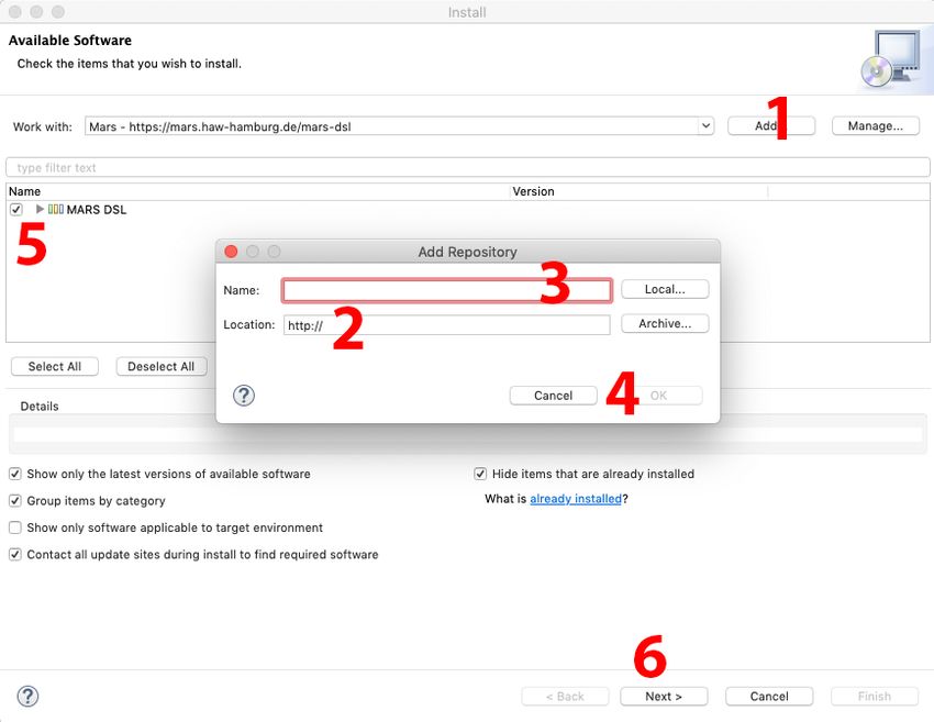
Multi-Agent Modelling with MARS: A Handbook

Release 1.7.2 (05.11.2019)

  • Add section about GeoJSON files to the cookbook part

  • Add section with examples about grid-layer CSV files to the cookbook

  • Update all code snippets, minor corrections

  • Extend section about movement with bearings and directions

Release 1.7.1 (04.11.2019)

  • Add section about ”use Mars” to language reference about the included math functions and constants

  • Extend movement sections to reflect the directional movement of agents

  • Add section about time-series files in conjunction with the raster-layer

  • Simulation config section contains table with available parameters now

  • Write about agent positioning out of agent init CSV files

  • Create new title page with logos of MARS group and HAW

Release 1.7 (30.10.2019)

  • Add new grid-layer for grid-based models (introduction + language reference)

  • Extend vector layer in language reference. More details about how to use it and new code examples

  • Update raster layer section in language reference with newest capabilities

  • Add section about advanced structuring of models in multiple files

  • Add sections about enums, arrays, maps and lists in the cookbook section

  • Completely rewrite ”MARS Models” chapter to reflect latest extensions. Mainly affects handling of
    layers (layer, grid-layer, raster-layer and vector-layer).

  • Update the whole handbook as the changes in coordinate systems affect most of it

Release 1.6.1 (10.10.2019)

  • Add details about explore operations with predicates

                                                                                          Page 2 of 57
Multi-Agent Modelling with MARS: A Handbook
Contents
1 Foreword and Installation 1
2 MARS Models 3
2.1 MARS . . . . . . . . . . . . . . . . . . . . . . . . . . . . . . . . . . . . . . . . . . . . . . . . . 3
2.2 From Technical Model to MARS Model . . . . . . . . . . . . . . . . . . . . . . . . . . . . . . 3
2.2.1 Different kind of models . . . . . . . . . . . . . . . . . . . . . . . . . . . . . . . . . . . 3
2.2.2 Starting Position . . . . . . . . . . . . . . . . . . . . . . . . . . . . . . . . . . . . . . . 3
2.2.3 Creating the Model Structure . . . . . . . . . . . . . . . . . . . . . . . . . . . . . . . . 4
2.2.4 Advanced Model Structure . . . . . . . . . . . . . . . . . . . . . . . . . . . . . . . . . 4
2.3 Layers . . . . . . . . . . . . . . . . . . . . . . . . . . . . . . . . . . . . . . . . . . . . . . . . . 4
2.3.1 Creating basic Layers . . . . . . . . . . . . . . . . . . . . . . . . . . . . . . . . . . . . 5
2.3.2 GIS layers . . . . . . . . . . . . . . . . . . . . . . . . . . . . . . . . . . . . . . . . . . . 5
2.3.3 Time-series layers . . . . . . . . . . . . . . . . . . . . . . . . . . . . . . . . . . . . . . . 5
2.4 Agents . . . . . . . . . . . . . . . . . . . . . . . . . . . . . . . . . . . . . . . . . . . . . . . . . 6
2.4.1 Creating Agents . . . . . . . . . . . . . . . . . . . . . . . . . . . . . . . . . . . . . . . 6
2.4.2 Agent Attributes . . . . . . . . . . . . . . . . . . . . . . . . . . . . . . . . . . . . . . . 7
Variables . . . . . . . . . . . . . . . . . . . . . . . . . . . . . . . . . . . . . . . . . . . 7
2.4.3 Positioning in grid-based models . . . . . . . . . . . . . . . . . . . . . . . . . . . . . . 7
2.4.4 Positioning in GPS-based models . . . . . . . . . . . . . . . . . . . . . . . . . . . . . . 7
2.4.5 Agent Behavior . . . . . . . . . . . . . . . . . . . . . . . . . . . . . . . . . . . . . . . . 8
Moving Agents . . . . . . . . . . . . . . . . . . . . . . . . . . . . . . . . . . . . . . . . 8
Finding other Agents . . . . . . . . . . . . . . . . . . . . . . . . . . . . . . . . . . . . . 9
Interactions between Agents . . . . . . . . . . . . . . . . . . . . . . . . . . . . . . . . . 10
Passive Actions . . . . . . . . . . . . . . . . . . . . . . . . . . . . . . . . . . . . 10
Active Actions . . . . . . . . . . . . . . . . . . . . . . . . . . . . . . . . . . . . 10
Message Passing . . . . . . . . . . . . . . . . . . . . . . . . . . . . . . . . . . . 11
2.4.6 Creating new Agents during Simulation . . . . . . . . . . . . . . . . . . . . . . . . . . 11
Agent States . . . . . . . . . . . . . . . . . . . . . . . . . . . . . . . . . . . . . . . . . 12
Life and Death: . . . . . . . . . . . . . . . . . . . . . . . . . . . . . . . . . . . . . . . . 12
2.5 Using GIS and time-series data . . . . . . . . . . . . . . . . . . . . . . . . . . . . . . . . . . . 13
2.5.1 Raster layer . . . . . . . . . . . . . . . . . . . . . . . . . . . . . . . . . . . . . . . . . . 13
2.5.2 Vector layer . . . . . . . . . . . . . . . . . . . . . . . . . . . . . . . . . . . . . . . . . . 14
2.5.3 Time-series capabilities . . . . . . . . . . . . . . . . . . . . . . . . . . . . . . . . . . . 15
3 Running simulations 17
3.1 Creating a simulation config . . . . . . . . . . . . . . . . . . . . . . . . . . . . . . . . . . . . . 17
3.1.1 Global parameters . . . . . . . . . . . . . . . . . . . . . . . . . . . . . . . . . . . . . . 18
3.1.2 Persisting results to a MongoDB (optional) . . . . . . . . . . . . . . . . . . . . . . . . 19
3.1.3 Data layers . . . . . . . . . . . . . . . . . . . . . . . . . . . . . . . . . . . . . . . . . . 19
3.1.4 Agent parameters . . . . . . . . . . . . . . . . . . . . . . . . . . . . . . . . . . . . . . 19
3.1.5 Agent initialization files . . . . . . . . . . . . . . . . . . . . . . . . . . . . . . . . . . . 20
3.2 Starting the simulation . . . . . . . . . . . . . . . . . . . . . . . . . . . . . . . . . . . . . . . . 20
3.2.1 Summary . . . . . . . . . . . . . . . . . . . . . . . . . . . . . . . . . . . . . . . . . . . 20
Page 3 of 57Multi-Agent Modelling with MARS: A Handbook
4 Language Reference 21
4.1 agent . . . . . . . . . . . . . . . . . . . . . . . . . . . . . . . . . . . . . . . . . . . . . . . . . . 21
4.2 distance . . . . . . . . . . . . . . . . . . . . . . . . . . . . . . . . . . . . . . . . . . . . . . . . 21
4.3 explore . . . . . . . . . . . . . . . . . . . . . . . . . . . . . . . . . . . . . . . . . . . . . . . . . 21
Explore basics . . . . . . . . . . . . . . . . . . . . . . . . . . . . . . . . . . . . . . . . 22
Explore with predicate . . . . . . . . . . . . . . . . . . . . . . . . . . . . . . . . . . . . 22
Null Reference Exceptions . . . . . . . . . . . . . . . . . . . . . . . . . . . . . . . . . . 23
4.4 external . . . . . . . . . . . . . . . . . . . . . . . . . . . . . . . . . . . . . . . . . . . . . . . . 24
4.5 grid-layer . . . . . . . . . . . . . . . . . . . . . . . . . . . . . . . . . . . . . . . . . . . . . . . 26
4.5.1 Grid-layers with data . . . . . . . . . . . . . . . . . . . . . . . . . . . . . . . . . . . . 26
4.6 initialize . . . . . . . . . . . . . . . . . . . . . . . . . . . . . . . . . . . . . . . . . . . . . . . . 27
4.7 kill me . . . . . . . . . . . . . . . . . . . . . . . . . . . . . . . . . . . . . . . . . . . . . . . . . 28
4.8 layer . . . . . . . . . . . . . . . . . . . . . . . . . . . . . . . . . . . . . . . . . . . . . . . . . . 28
4.8.1 Layer Attributes and Functions . . . . . . . . . . . . . . . . . . . . . . . . . . . . . . . 28
4.9 move . . . . . . . . . . . . . . . . . . . . . . . . . . . . . . . . . . . . . . . . . . . . . . . . . . 29
4.9.1 Grid movement examples . . . . . . . . . . . . . . . . . . . . . . . . . . . . . . . . . . 30
4.9.2 Move with directions . . . . . . . . . . . . . . . . . . . . . . . . . . . . . . . . . . . . . 31
4.9.3 Move with bearing . . . . . . . . . . . . . . . . . . . . . . . . . . . . . . . . . . . . . . 31
4.10 nearest . . . . . . . . . . . . . . . . . . . . . . . . . . . . . . . . . . . . . . . . . . . . . . . . . 32
4.10.1 Nearest agent . . . . . . . . . . . . . . . . . . . . . . . . . . . . . . . . . . . . . . . . . 32
4.10.2 Nearest GIS feature . . . . . . . . . . . . . . . . . . . . . . . . . . . . . . . . . . . . . 32
4.10.3 Nearest with limited range . . . . . . . . . . . . . . . . . . . . . . . . . . . . . . . . . 32
4.10.4 Null Reference Exceptions . . . . . . . . . . . . . . . . . . . . . . . . . . . . . . . . . . 33
4.11 observe . . . . . . . . . . . . . . . . . . . . . . . . . . . . . . . . . . . . . . . . . . . . . . . . 33
4.12 pos at . . . . . . . . . . . . . . . . . . . . . . . . . . . . . . . . . . . . . . . . . . . . . . . . . 34
4.13 random . . . . . . . . . . . . . . . . . . . . . . . . . . . . . . . . . . . . . . . . . . . . . . . . 34
4.14 raster-layer . . . . . . . . . . . . . . . . . . . . . . . . . . . . . . . . . . . . . . . . . . . . . . 35
4.14.1 Reading information . . . . . . . . . . . . . . . . . . . . . . . . . . . . . . . . . . . . . 35
4.14.2 Changing values . . . . . . . . . . . . . . . . . . . . . . . . . . . . . . . . . . . . . . . 36
4.15 simtime . . . . . . . . . . . . . . . . . . . . . . . . . . . . . . . . . . . . . . . . . . . . . . . . 36
4.15.1 Simtime Example 1 . . . . . . . . . . . . . . . . . . . . . . . . . . . . . . . . . . . . . 36
4.15.2 Simtime Example 2 . . . . . . . . . . . . . . . . . . . . . . . . . . . . . . . . . . . . . 37
4.16 spawn . . . . . . . . . . . . . . . . . . . . . . . . . . . . . . . . . . . . . . . . . . . . . . . . . 38
4.17 static . . . . . . . . . . . . . . . . . . . . . . . . . . . . . . . . . . . . . . . . . . . . . . . . . . 38
4.18 tick . . . . . . . . . . . . . . . . . . . . . . . . . . . . . . . . . . . . . . . . . . . . . . . . . . . 38
4.19 use MARS . . . . . . . . . . . . . . . . . . . . . . . . . . . . . . . . . . . . . . . . . . . . . . . 39
4.20 val . . . . . . . . . . . . . . . . . . . . . . . . . . . . . . . . . . . . . . . . . . . . . . . . . . . 39
4.21 var . . . . . . . . . . . . . . . . . . . . . . . . . . . . . . . . . . . . . . . . . . . . . . . . . . . 40
4.22 vector-layer . . . . . . . . . . . . . . . . . . . . . . . . . . . . . . . . . . . . . . . . . . . . . . 40
4.22.1 Reading information . . . . . . . . . . . . . . . . . . . . . . . . . . . . . . . . . . . . . 41
4.22.2 Changing values . . . . . . . . . . . . . . . . . . . . . . . . . . . . . . . . . . . . . . . 41
4.22.3 Working with the vector layer . . . . . . . . . . . . . . . . . . . . . . . . . . . . . . . . 41
4.23 x-cor and ycor . . . . . . . . . . . . . . . . . . . . . . . . . . . . . . . . . . . . . . . . . . . . 42
5 Cookbook 43
5.1 Example Models . . . . . . . . . . . . . . . . . . . . . . . . . . . . . . . . . . . . . . . . . . . 43
5.1.1 Wolf, Sheep, Grass . . . . . . . . . . . . . . . . . . . . . . . . . . . . . . . . . . . . . . 43
5.1.2 Chatting Agents . . . . . . . . . . . . . . . . . . . . . . . . . . . . . . . . . . . . . . . 46
5.2 Useful Code Snippets . . . . . . . . . . . . . . . . . . . . . . . . . . . . . . . . . . . . . . . . . 47
Page 4 of 575.2.1 Agent Evolution . . . . . . . . . . . . . . . . . . . . . . . . . . . . . . . . . . . . . . . 47
5.2.2 Agent Live Stages . . . . . . . . . . . . . . . . . . . . . . . . . . . . . . . . . . . . . . 47
5.2.3 Random Walk . . . . . . . . . . . . . . . . . . . . . . . . . . . . . . . . . . . . . . . . 48
5.2.4 Biomass Removal . . . . . . . . . . . . . . . . . . . . . . . . . . . . . . . . . . . . . . . 48
5.2.5 Agent Interaction: Buying Goods . . . . . . . . . . . . . . . . . . . . . . . . . . . . . . 49
5.3 Data Usage Examples . . . . . . . . . . . . . . . . . . . . . . . . . . . . . . . . . . . . . . . . 50
5.3.1 Agent Init Files . . . . . . . . . . . . . . . . . . . . . . . . . . . . . . . . . . . . . . . . 50
5.3.2 CSV files for grid-layer . . . . . . . . . . . . . . . . . . . . . . . . . . . . . . . . . . . . 51
5.3.3 ASC files for raster-layer . . . . . . . . . . . . . . . . . . . . . . . . . . . . . . . . . . . 51
5.3.4 GeoJSON files for vector-layer . . . . . . . . . . . . . . . . . . . . . . . . . . . . . . . 52
5.3.5 Time-series files . . . . . . . . . . . . . . . . . . . . . . . . . . . . . . . . . . . . . . . . 52
5.4 Programming Features . . . . . . . . . . . . . . . . . . . . . . . . . . . . . . . . . . . . . . . . 53
5.4.1 Functions . . . . . . . . . . . . . . . . . . . . . . . . . . . . . . . . . . . . . . . . . . . 53
5.4.2 Arrays . . . . . . . . . . . . . . . . . . . . . . . . . . . . . . . . . . . . . . . . . . . . . 54
5.4.3 Enums . . . . . . . . . . . . . . . . . . . . . . . . . . . . . . . . . . . . . . . . . . . . . 54
5.4.4 Lists . . . . . . . . . . . . . . . . . . . . . . . . . . . . . . . . . . . . . . . . . . . . . . 55
5.4.5 Maps/ Dictionaries . . . . . . . . . . . . . . . . . . . . . . . . . . . . . . . . . . . . . . 55
5.4.6 Loops . . . . . . . . . . . . . . . . . . . . . . . . . . . . . . . . . . . . . . . . . . . . . 56
for loops . . . . . . . . . . . . . . . . . . . . . . . . . . . . . . . . . . . . . . . . . . . . 56
foreach loops . . . . . . . . . . . . . . . . . . . . . . . . . . . . . . . . . . . . . . . . . 56
while loops . . . . . . . . . . . . . . . . . . . . . . . . . . . . . . . . . . . . . . . . . . 56
Example: Observer agent use loop to iterate over all raster cells . . . . . . . . . . . . . 57Multi-Agent Modelling with MARS: A Handbook
1 Foreword and Installation
Welcome to the modeling handbook on agent-based models with MARS. This will be an introduction to
multi-agent modeling, the technical details during model implementation and the simulation execution. In
order to work with the handbook you will have to install the following programs:
All programming is going to be done in Eclipse. Before you can use Eclipse to build MARS models you have
to install the JAVA software development kit. Once JAVA has been installed and Eclipse opened you can
add MARS functionality to it by installing our Eclipse plugin.
• Dotnet Core https://dotnet.microsoft.com/download/dotnet-core/2.2
You will need to download the SDK (Version 2.2.402)
• JAVA SDK https://www.oracle.com/technetwork/java/javase/downloads/index.h
tml
• Eclipse https://www.eclipse.org/downloads/
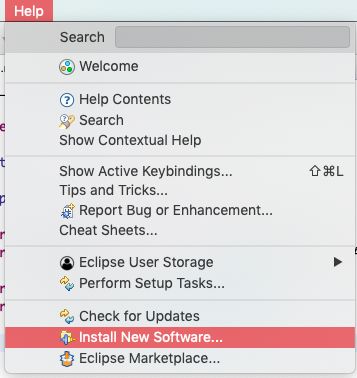
To install the MARS plugin you have to open Eclipse. On both MacOS and Windows you can find the
’Install New Software’ menu under ’Help’ as shown in figure 1. Once you open the window it will look like
figure 2 without the pop-up. The first step is to add the MARS plugin URL to Eclipse. Click on the ’Add’
field marked with a red one in figure 2. Step number two is the following URL to the field marked with two:
• MARS Plugin https://mars.haw-hamburg.de/mars-dsl/
For ’name’ you can put MARS (marked with three), then press ’ok’. Now you should see the entry above
the red number five where it says ’MARS
DSL’. Check the checkbox and press ’next’
marked by the red six. After this you will
be lead through the installation process by
Eclipse. You might be prompted an error that
the certificates couldn’t be checked for the plu-
gin. Should this happen, press ”install any-
way” to proceed with the installation. After
successful installation you will be asked restart
Eclipse. Once this has been done, you are
ready to program your first MARS multi-agent
model.
After programming the model in Eclipse, Dotnet
Core will be needed to build and execute the model.
If you encounter any problems you can contact us
through our Slack system. You can join via the fol-
lowing link:
Figure 1: Eclipse: installing new software mars-explorers.slack.com
Page 1 of 57Multi-Agent Modelling with MARS: A Handbook
Figure 2: Installing the MARS DSL plugin to Eclipse part 2
Page 2 of 57Multi-Agent Modelling with MARS: A Handbook
2 MARS Models
Agent based modeling derives from the field of artificial intelligence. This simulation paradigm incorporates
individuals, so called agents, who interact with each other and their surroundings. The behavior is pro-
grammed on an individual level to follow a set of rules and interactions between them are studied to gain
insights into collective behavior [2]. Note that an agent isn’t restricted to be an individual but can also be
a group, community or other entity that acts and reacts to outer conditions [4]. The way of creating results
bottom-up from an individual levels actions leading to complex effect makes it especially suited for research
on social sciences [1].
This handbook is designed to be an introduction for people who are new to multi-agent modeling, program-
ming in general and the MARS framework.
2.1 MARS
The multi-agent framework MARS (Multi-Agent Research and Simulation) is a research project, developed at
the University of Applied Sciences Hamburg [5]. Incorporating newest concepts of agent-based and individual-
based programming [6]. The frameworks targets both simple and complex models by using specifically
designed approaches tailored to the respective disciplines like for example social ecology [3].
2.2 From Technical Model to MARS Model
Throughout this handbook we are going to use a custom domain specific language (DSL) for programming.
Daniel Glake, a member of the MARS group, created this language which targets socio-ecological models.
To make the introduction easier, we will implement an example model over the course of this handbook.
This model is going to be a simple predator-prey scenario consisting of three agent types: wolves, sheep and
grass. Each Agent is considered a living entity that has to eat in order to stay alive. For the wolves this
means that they have to eat sheep and the sheep have to eat grass. Wolves and sheep agents can reproduce.
If they have eaten enough, they eventually hatch an offspring. The grass periodically grows back on its own.
2.2.1 Different kind of models
Please read the following paragraph carefully and make sure you understand it before continuing to work
with the handbook. There are two types of models in MARS: grid-based ones and GPS-based ones. Their
biggest distinction is between using a grid as coordinate reference system or GPS (geospatial models). The
two are not compatible as they target different kind of models. You will have to choose the appropriate one
depending on your use-case.
If you want to create a simple model where the agents move around on a grid and interact with each other
you should choose the grid as your coordinate reference system. Should you on the other hand wish to do a
more complex model that might even include GIS data or time-series data you should opt for the GPS-based
one. The agents will still be able to move around and interact but they will use longitude and latitude values
as their means of positioning and distances will be in meters instead of grid cells.
The example model of wolf, sheep and grass will be realized as a grid-based model to showcase the systems
capability in an easy to understand way.
2.2.2 Starting Position
Every model needs to start somewhere. This is usually a class diagram which already covers the models
agents and layers. The authors expect that you are familiar with conceptual modeling at this point of reading
and have a valid design model at hand. From there you can follow this handbook to transform the existing
Page 3 of 57Multi-Agent Modelling with MARS: A Handbook
technical model, that is what the model ideas on paper are being called, to a working piece of code. This is
the actual model which will be executed on the MARS platform.
2.2.3 Creating the Model Structure
New models follow a set of formatting rules that enable the computer to understand them. Generally
speaking the models are divided into three groups:
1. model definition
2. layer definition
3. agent definition
These are the building blocks for any model idea. So when you as a modeler start implementing your model
with the MARS DSL, this is the pattern you have to stick to.
Model definition happens in the first line of every model. Listing 1 demonstrates this by creating a model
in line 0 with the name wolf sheep grass. When creating your own model, this is where the name of your
model is going to be put.
In line 2 the models layers are created. For this simple model it is going to be a single grid-layer with the
name of AgentLayer. We use a grid-layer because the model doesn’t need to have a geo-reference which
would make things unnecessarily complicated. While implementing models every layer must be created after
the model definition and before the agent definitions.
The agent definition happens in line 4. Agents are defined by giving them a name and specifying on which
layer they are going to live. For this model the first agent has the name wolf and will be managed by the
layer with name AgentLayer that has been created before. The same is done for the sheep and grass agents
in lines five and six.
0 model wolf_sheep_grass
1
2 grid - layer AgentLayer as agentlayer
3
4 agent wolf on AgentLayer{}
5 agent sheep on AgentLayer{}
6 agent grass on AgentLayer{}
Listing 1: Basic model structure
2.2.4 Advanced Model Structure
Should you wish to distribute your code over multiple files, you can do so. It is possible to write one agent
type in file 1 and another one in file 2. They will still be able to interact. All you have to do is create another
”.mars” file in the ”src” folder. In the first line of all files the model name must be the same, otherwise it
wont work.
2.3 Layers
Layers in MARS are instruments to fulfill the tasks of agent management or data management. Depending
on your model, you will be using one or several different layer types.
Page 4 of 57Multi-Agent Modelling with MARS: A Handbook
Baseline are the layers to manage agents. They are called that because they will contain the respective
agents and manage their movements. If your model is grid-based the layer will have to be a grid-layer in
order to work. This allows the agents to move on a grid whose size you get to define. The basic layer (
layer ) is for those who wish their model to be GPS-based. It can manage agents in the same way as the
grid-layer can with the difference that the movements will be based on longitude and latitude. At least one
of these layers will be present in every model but never both at the same time as layer and grid-layer are
not compatible.
GIS layers with and without time-series capabilites are designed to provide GIS and time-series functionality.
They can be included to access such data during simulations. As they rely on GPS as reference system, they
are not compatible with grid-layers .
Grid-layers have a special feature that regular layers don’t have: they can contain rasterized data without
a spatial reference. Basis for this are CSV files that make up a grid with each entry representing one grid
cell worth of information. The section CSV files for grid-layer (5.3.2) descibes these files in detail and the
grid-layer (4.5) section demonstrates the usage in an example model.
1. Layer Used in GPS-based models to manage agents
2. Grid-Layers Used for grid-based models to manage agents and to represent rasterized data
3. GIS Raster Layers Used to provide access to rasterized GIS data, cannot manage agents
4. GIS Vector Layers Offer access to vector GIS data and time-series data, cannot manage agents
2.3.1 Creating basic Layers
Now that you know the basics about layers, it is time to create the ones that your model includes. First you
have to decide on the coordinate reference system. If your model is grid-based the agents will be managed
on a grid-layer . Otherwise you should choose the layer to handle everything agent related. Think of a
name that describes the agents surroundings and create such a layer as shown in listing 2 in line 0. In the
example the layer has the name AgentLayer, name yours according to what you have thought of. The name
has no effect on the model behavior.
2.3.2 GIS layers
Once the basic layers have been setup, you continue with the optional GIS layers and time-series layers.
These layers can be created like shown in listing 2. The MARS DSL allows to use ASC and GeoJSON files.
The keyword for GIS raster layers is raster-layer followed by the name the layer should have and an alias
which we will use to refer to the layer later in the model. For these two names (GisVegetationLayer and
gisvegetationayer in the example) it is customary to give them the same name. Write the first one in camel
case and the second one in lower case. Again, the names have no effect on the model.
For GIS vector layers the procedure works accordingly with the vector-layer keyword.
2.3.3 Time-series layers
Time-series layers are created similar to the GIS layers since their functionality is provided through the
raster-layer . Line 6 of listing 2 shows a raster-layer that is being used to provide time-series data about
temperature values to the agents during the simulation. More information about the use of time-series can
be found in the next section.
Page 5 of 57Multi-Agent Modelling with MARS: A Handbook
0 layer AgentLayer
1
2 raster - layer GisVegetationLayer as gisvegetationlayer
3
4 vector - layer WaterPointLayer as waterpointlayer
5
6 raster - layer TemperatureLayer as temperaturelayer
Listing 2: Available Layer types
2.4 Agents
Agents are the main part of every model (besides layers). Once the layers have been created, we can start
specifying the the agents. For this step you, as a modeler, need to know what your agents are going to be,
what attributes define them and what their actions will look like. Once this has been established, we can
start with the agent creation.
To illustrate the agent creation process, we will continue with the wolf, sheep, grass example model that was
described in the introduction. First this model will be described in detail, then the agents are going to be
created throughout this part of the handbook. The wolf, sheep, grass model consists of three agent types
one layer to manage them. All agent types (wolves, sheep and grass) will be living on the basic layer:
Wolf Agent This agent moves around the simulated area and tries to find sheep agents in order to feed
on them. When he catches one, he eats it, thereby increasing his energy level. If the wolf can’t find
sheep for a period of time, it dies. If the wolf eats enough sheep agents, he can reproduce which leads
to new wolf agents in a juvenile state. Wolves in that state have a reduced amount of energy and are
therefore more likely to die.
Sheep Agent This agent type moves around the simulated area as well. His objective is to find grass that
can be eaten. Upon eating grass the sheep increases its energy level. Like the wolf agent, the sheep
can reproduce when they eat enough grass. If the sheep agent can’t find grass for an extended period
of time, it dies.
Grass Agent The last of the three agents is mainly a food target for the sheep. Grass agents stay at one
place and grow back once they have been eaten. They are distributed randomly around the simulated
area.
2.4.1 Creating Agents
With the wolf, sheep and grass model in place, it is time to create the agents. Listing 3 shows this step.
It starts with a model definition in line 0, this should be familiar from the introduction. Next we define a
grid-layer with the name AgentLayer that will serve to manage the agents. From line 4 on we create the
three agent types, starting with the wolf. The keyword for creating agents is agent . It is followed by the
name of the agent and a layer allocation. This layer allocation tells the model on which layer the agents are
going to live. For the wolf this is going to be the AgentLayer that we defined above. Note the curly braces
at the end of line 5, these will later enclose the agent’s attributes and behavior. More about this in the next
section. For the sheep and grass agents we do the same as for the wolf. Each agent type has to be defined,
receives a name and is told to live on the AgentLayer.
Page 6 of 57Multi-Agent Modelling with MARS: A Handbook
0 model wolf_sheep_grass
1
2 grid - layer AgentLayer as agentlayer
3
4 agent wolf on AgentLayer{}
5 agent sheep on AgentLayer{}
6 agent grass on AgentLayer{}
Listing 3: Creating wolf and sheep agents
2.4.2 Agent Attributes
Agents have a set of attributes that define their state. These attributes are defined through variables
inside the agents curly braces as shown in listing 4. Variables can be thought of as little boxes that store
information. For each of the agents attributes like age, energy etc. we define one of those variables that can
later be worked with or altered during simulation execution.
Variables can be of different types. MARS supports integers, floating point numbers (reals), boolean
values and strings - for those familiar with programming. Listing 4 shows an example for these variables
and how they are defined in the MARS DSL. Integer variables can store integers (numbers without floating
point) whereas real variables can save floating point numbers. Boolean values allow a binary distinction
between true and false. The last type of variables are strings which are useful to store text or characters.
0 agent wolf on AgentLayer {
1 var Energy : integer = 10
2 var Weight : r e a l = 70
3 var Name : string = "Wolf"
4 }
Listing 4: Creating attributes of each available type
2.4.3 Positioning in grid-based models
Agents will be positioned on a grid that makes up the simulation space. The grid size can be set by you so it
can be as small or big as you need it to be. In the standard configuration the grid will have the dimionsions
100x100 cells. Origin of the grid is the lower left corner which corresponds to position (0/0). From there the
grid spans in x- and y-direction to the specified size. Movements on the grid and distances are measured in
grid cells. Figure 3 shows an example with 100 by 100 grid cells. Please note that the grid system starts
with coordinate (0/0) and not with (1/1). This means that in a grid with 10x10 cells there is no (10/10)
coordinate. The furthest you can go is (9/9).
2.4.4 Positioning in GPS-based models
Instead of grid cells the GPS-based coordinate system works with longitude and latitude as coordinates. If
you choose to work with this system your movements and distances will be in meters and your positioning
will be GPS coordinates. You can read more about this so called ”global positioning system” here.
Page 7 of 57Multi-Agent Modelling with MARS: A Handbook
Figure 3: Example grid with 100 by 100 cells
The two kinds of positioning are not compatible so you have to choose which one you want. For first
time modelers the grid is recommended as this makes the model easier to understand. GPS allows for
more complex models but it increases the level of difficulty as well.
2.4.5 Agent Behavior
All agents follow a set of rules that define their behavior. In each simulation step the agents get to perform
these actions. The behavior (actions) is specified inside the curly braces of the agents tick method. As agent-
based simulations are time-discrete, this repeats over and over until the simulation is finished. Listing 5 shows
an agent creation with the tick method (line 2) to specify the agent’s behavior. All of the agent logic with
its instructions is stored there. More information about the tick method can be found in section tick (4.18)
The initialize method is executed before the first tick . Its purpose is to initialize the agent’s variables.
This special method is equivalent to a constructor and will only be called exactly once. You can find more
information in the initialize (4.6) section.
0 agent wolf on AgentLayer{
1 i n i t i a l i z e {}
2 t i c k {}
3 }
Listing 5: Agent definition with initialize and tick methods
Moving Agents One of the most basic actions an agent can perform is movement. This is simply the way
of changing an agents position from one point to another. This works independent of the chosen coordinate
Page 8 of 57Multi-Agent Modelling with MARS: A Handbook
system. Movement actions can be performed in various levels of sophistication ranging from small reposi-
tioning to complex pathfinding operations to avoid obstacles.
A basic move operation consists of four parts starting with the actual move command ( move ). Next you
have to specify what you want to move. For most situations this will be the agent itself but it is also possible
to move other agents. If you want to move the agent itself you write me after the move command. This
tells the system that you want to move the agent itself.
From here you have to decide whether you want to move the agent in a specific direction or towards a desti-
nation. For movements to a certain destination you have to write the to keyword after which you have to
specify a coordinate. These have to be written in the DSL specific coordinate notation as shown in listing 6.
This notation starts with a hash symbol and braces that enclose the x and y-coordinates, separated through
a comma. These coordinates can be grid coordinates or GPS coordinates, depending on your model. In
line 0 the agent is told to move to position (1/5). Optionally a distance can be specified, telling the agent
how far he should move. If your model is based on a grid this distance will be in grid-cells, otherwise it will
be meter for GPS models. Line 1 shows how an agent can be moved three grid cells in the direction of (10/15).
Another type of movement is direction based. This can be seen in line three of listing 6 where the agent is
told to move 5 grid cells/ meters to the right. Possible directions are: up, up-right, right, down-right, down,
down-left, left and up-left.
Line 3 shows a movement operation in conjunction with a bearing. The agent is told to move towards 180
degree which means going down. 0 degree is up (north), 90 degree is right (east), 180 degree is down (south)
and 270 degree is left (west).
0 move me to #(53.55,10.01)
1 move me 3 to #(10,15)
2 move me 5 right
3 move me to 180
Listing 6: Example move commands
Finding other Agents Before agents move, they usually plan where to go. This is where so called
”exploration” operations come into play. These actions allow to find other agent to engage or to interact
with their environment. For the wolf, sheep, grass model this means locating each other. Before the wolf
agent can eat a sheep, it first has to find one and then move there.
In general, agents can be located through explore or nearest operations on the environment/ layers.
Listing 7 shows the nearest command in combination with a variable. This variable (nearestSheep) saves
the nearest sheep’s position and is used as input for the move command afterwards. The nearest command
always provides the closest agent of the desired type. In listing 7 the specified type was sheep. This works
as long as there are sheep present in the simulation. Once all sheep are gone, the nearest command will
crash the simulation. This happens because the nearest command can only return a valid position if there
is something to find. If there are no sheep left, the nearest command returns an empty coordinate that the
move command can’t handle. Since the ”there” doesn’t exist, the computer doesn’t know what to do. More
details on this topic and how to avoid the problems can be found in the nearest (4.10) section.
0 agent wolf on AgentLayer{
1
2 tick{
3 var nearestSheep = nearest sheep
Page 9 of 57Multi-Agent Modelling with MARS: A Handbook
4 move me to nearestSheep
5 }
6 }
Listing 7: Wolf agent searching for the nearest sheep and moving there
Interactions between Agents As of now we are able to locate other agents and move around the
simulated space. The interesting part of multi-agent models starts when agents interact. Either with each
other or with their environment.
Direct interactions between agents consist of an active and a passive part called ”active actions” and ”passive
actions”. The initiating agent does the active part whereas the chosen partner-agent takes the passive role.
Before the active agent can perform an interaction, the passive agent has to specify what such an interaction
means to him.
In our example model, when a wolf eats a sheep, the wolf is the active agent and the sheep is the passive
partner. The sheep, which is about to be eaten, has to determine what effect that has. From a human
perspective it is clear that the sheep would die but the model has to be told that explicitly. The next section
introduces this process in detail.
Passive Actions define the effects of an interaction to the passive agent. The passive agent is the one on
which the action is performed on. To give an example we will program the passive action part of an wolf -
sheep interaction where the sheep will be eaten (listing 8). Passive actions are part of the agent in the agent
and start with the passive keyword, followed by the name of the interaction. These methods look similar to
an agents tick method with the difference that they are not executed in every simulation step. Parentheses
after the method name enclose potential input arguments and the main part of the passive actions follows
inside curly braces afterwards. In the case of the sheep we devise a passive action with the name BeEaten
that takes no input parameters. Enclosed in the curly braces follows the statement that the sheep dies (line
3). This concludes the passive action that can now be used by other agents.
0 agent sheep on AgentLayer{
1 t i c k {}
2 passive BeEaten(){
3 k i l l me
4 }
5 }
Listing 8: Sheep passive action
Active Actions Once passive actions have been defined, the other half of interactions can be performed:
the active part. Agents that want to initiate an interaction must select an agent before they can interact. In
the wolf, sheep, grass model that means that a wolf has to select a sheep first before he can eat it. Listing
9 shows that process where the the wolf locates the closest sheep in line 2 and then moves there. Note that
we didn’t check if the wolf and the sheep are close by, we’ll do that in a later example. For now it is more
important focus on line 4 where the just implemented passive BeEaten action of the sheep is being called.
The wolf initiates the interaction thereby forcing the sheep to react in the specified way. As a result the
sheep dies and the wolf has successfully eaten a sheep.
0 agent wolf on AgentLayer{
1 tick{
Page 10 of 57Multi-Agent Modelling with MARS: A Handbook
2 var nearestSheep = nearest sheep
3 move me to nearestSheep
4 nearestSheep.BeEaten()
5 }
6 }
Listing 9: Wolf eating the nearest sheep
Message Passing Now that you know how agents find and interact with each other, the ability to com-
municate might be desired. Agents can communicate directly or via a proxy in form of a layer. Direct
communication is best suited for scenarios in which exactly two agents want to exchange messages. If more
than two agents want to communicate, the latter approach is the way to go. Communication over a layer
follows the idea of a blackboard where agents can leave each other messages and react to them. If you want
your agents to use a message based approach, take a look at Chatting Agents (5.1.2) in the cookbook
section where this example model is explained. The model uses message-passing through a layer so that two
agent types can communicate with each other.
2.4.6 Creating new Agents during Simulation
For situations where new agents have to be created during simulation, the spawn command can be used. A
recurring use-case would be for agents to reproduce over the course of the simulation. The spawn commands
creates a new agent with its own variables and methods. A completely new agent, independent of the creating
one. In the wolf, sheep, grass model this is used when wolves or sheep reproduce. Pre-requirement (in the
model) for such a reproduction is that the wolf or sheep has eaten enough so that its energy level is high
enough. Listing 10 shows the code. In line 7, the wolf checks if it has enough energy and eventually spawns
a new wolf. This process costs him half of its energy so that is has to eat others sheep before being able to
reproduce again. Be careful with this kind of reproduction as it can easily produce exponential growth if
not controlled correctly. Can you spot the problem with the code?
0 agent wolf on AgentLayer{
1 var energy = 5
2 tick{
3 var nearestSheep = nearest sheep
4 move me to nearestSheep
5 nearestSheep.BeEaten()
6 energy = energy + 5
7 i f (energy > 20){
8 spawn wolf
9 energy = energy / 2
10 }
11 }
12 }
Listing 10: Wolf agent spawning new agents
Initially the wolf has an energy level of 5. In the fifth line the wolf eats a sheep (even if it isn’t close) and
then adds 5 to his energy level. So after the first simulation step the wolf already has an energy level of
10. Two steps later the wolf has enough energy to reproduce (on its own, no partner needed). A new wolf
is created and the old one reduces its energy to 10. After two more steps the old wolf has replenished its
Page 11 of 57Multi-Agent Modelling with MARS: A Handbook
energy and is reproduce again. So at simulation step five we already have 3 wolves. One step later, the other
wolf that was created in step 3 has enough energy to reproduce as well resulting in 4 wolves in step six. You
see where this is going so be just be careful with your own code.
Agent States can be used to set different behavior for different agent conditions. The states can be
age-related like juvenile and adults or can refer to an energy level etc. Depending on its current state, the
agent changes his behavior.
Listing 11 show this for the wolf agent. Two states (0 and 1) determine whether the wolf is an juvenile or
an adult. During the simulation the wolf acts accordingly (line 8 for juvenile and line 12 for adult). Once
the simulation reaches its 50th step, the agent’s state changes from juvenile to adult.
0 agent wolf on AgentLayer{
1 var agentState : integer = 0
2
3 tick{
4 i f (simtime > 50){
5 agentState = 1
6 }
7 // juvenile state
8 i f (agentState === 0){
9 //act as juvenile
10 }
11 // adult state
12 else{
13 // behave like an adult
14 }
15 }
16 }
Listing 11: Wolf agent with two states
Life and Death: Agents will be removed from a simulation once they die. All agents are mortal and can
be killed in any simulation step by using the kill command. Listing 12 shows the wolf agent dying when
its Energy level falls to 0. If this condition is true, the agent uses the kill command in combination with
the me to signal the MARS system that is dead now.
0 agent wolf on AgentLayer {
1 var Energy : integer = 100
2 tick{
3 Energy = Energy - 1
4 i f (EnergyMulti-Agent Modelling with MARS: A Handbook
The model works like this: In every simulation step, the wolfs energy is reduced by 1. After 100 simulation
steps, the energy will be zero and the wolf will be removed from the simulation. You can read up on the file
types in the following sections:
• ASC files for raster-layer (5.3.3)
• GeoJSON files for vector-layer (5.3.4)
• Time-series files (5.3.5)
2.5 Using GIS and time-series data
Interactions with the Environment aren’t the same as those among agents. These interactions consist of
predefined actions, offered by the raster-layer and vector-layer . Agents can call these to read from the
environment or to alter it. These GIS layers allow to use a range of GIS files in the simulation which are
limited to ASC files (for the raster layer) and GeoJSON files (for the vector layer). Data in other formats
has to be converted to one of these, otherwise you cannot make use of them.
To use the GIS data in your model you either have to create a raster-layer or a vector-layer . If you’re
unsure which one to use, you can read up on each of them in the language reference at 4.14 for raster-layer
and at 4.22 for the vector-layer . The actual GIS file will be added later in the simulation config before
starting the simulation.
2.5.1 Raster layer
Listing 13 demonstrates the creation and use of the raster-layers . In line 3 such a layer by the name of
”BiomassLayer” is created. In addition to the name of the layer itself you have to specify an alias by which
the layer is referred to in the code. One of the easiest ways of working with the raster-layer is to find
the nearest raster containing information. Information is any value that is not equal to the ”no-data” value
specified in the ASC input file. This can be seen in line 7 where the wolf agents tries to find the closest cell
on the ”biomass-layer”. The nearest command returns the position which can then be used as destination
for the move command to get there.
Next up are the predefined methods offered by the raster-layer (lines 10–24). The first group (line 10–14)
allows to read information from the layer in varying formats. All of them have in common that you have
to specify the coordinate (grid or GPS) from which you want to read the information. Use the appropriate
method based on what kind of information is contained in you input files.
Lines 16 to 19 demonstrate how to query the raster-layer for its boundaries. The four commands allow to
check the dimensions of the layer, represented by its bounding box.
Agents can also alter the contained information. In the same way as for the reading access they have
to specify the coordinate of the grid cell they want to change the values for. To reduce or increase the
current value the designated methods ”Increase()” and ”Reduce()” have been included. Overwriting the
value completely can be done with the methods shown in line 23 and 24. Note that you will have to provide
the desired new value in addition to the coordinates.
0 model wolf_sheep_grass
1
2 layer AgentLayer
3 raster - layer BiomassLayer as biomasslayer
Page 13 of 57Multi-Agent Modelling with MARS: A Handbook
4
5 agent wolf on AgentLayer{
6 tick{
7 var position = nearest on BiomassLayer
8 move me to position
9
10 var boolValue = biomasslayer.GetBoolValue( xcor , ycor )
11 var intValue = biomasslayer.GetIntegerValue( xcor , ycor )
12 var realValue = biomasslayer.GetRealValue( xcor , ycor )
13 var stringValue = biomasslayer.GetStringValue( xcor , ycor )
14 var value = biomasslayer.GetValue( xcor , ycor )
15
16 var maxLat = biomasslayer.MaxLat()
17 var maxLon = biomasslayer.MaxLon()
18 var minLat = biomasslayer.MinLat()
19 var minLon = biomasslayer.MinLon()
20
21 biomasslayer.Increase( xcor , ycor , 1)
22 biomasslayer.Reduce( xcor , ycor , 1)
23 biomasslayer.SetIntegerValue( xcor , ycor , 1)
24 biomasslayer.SetRealValue( xcor , ycor , 1.0)
25 }
26 }
Listing 13: Working with the raster-layer
2.5.2 Vector layer
For this example we will a vector-layer called ”waterpointlayer” (line 3). It contains information about
the positions of water-points in the simulated area. The first use-case for the layer would be to find the
closest one. This can be seen in line 7 where the wolf agent uses the nearest command to query the
”waterpointlayer” for the closest position. In the next step the wolf moves there (line 8).
To read information from vector-layers you can use the ”Get()” commands that are shown in lines 10 and
11. Vector datasets contain so called ”features” which represent the contained information. Each vector-
layer can contain multiple features so there might be more than one kind of information represented. The
simple ”Get()” method in line 10 addresses the situation where there is only one feature present. It will
directly return the read information from the layer. Should your dataset contain multiple features, you will
have to use option number two in line 11. In addition to the coordinates you will also have to specify the
name of the feature you want to read information from.
Lines 13 to 16 demonstrate how to query the vector-layer for its boundaries. The four commands allow to
check the dimensions of the layer, represented by its bounding box.
0 model wolf_sheep_grass
1
2 layer AgentLayer
3 vector - layer WaterpointLayer as waterpointlayer
Page 14 of 57Multi-Agent Modelling with MARS: A Handbook
4
5 agent wolf on AgentLayer{
6 tick{
7 var position = nearest on WaterpointLayer
8 move me to position
9
10 var a = waterpointlayer.Get( xcor , ycor )
11 var b = waterpointlayer.Get( xcor , ycor , "test")
12
13 var maxLat = waterpointlayer.MaxLat()
14 var maxLon = waterpointlayer.MaxLon()
15 var minLat = waterpointlayer.MinLat()
16 var minLon = waterpointlayer.MinLon()
17 }
18 }
Listing 14: All methods of the vector-layer
2.5.3 Time-series capabilities
If you wan’t to use time-series data in your model you will be using a raster-layer to represent that infor-
mation. Read more about the compatible input files in the Time-series files (5.3.5) section. For every
simulation step, the layer will return the current value for that point in time.
The example model uses temperature data that changes throughout the simulation. For this, a new raster-
layer with the name ”TemperatureLayer” is created in line 3. The information in that layer will be updated
as specified in the provided input file. For now it is only important to understand that the returned informa-
tion changes over the course of the simulation so that the agents are always working with the appropriate data.
Querying the information can be done by using one of the five methods shown in lines 7 to 11 of listing
15. Depending on the used method, the contained information formatted as boolean, integer, real or string
value. If you know in which format the data is contained in your input file you can also use the ”GetValue()”
methods which returns the information without formatting it. So if you call the method in line 9, the wolf
agent will receive the current temperature value for that simulation step.
0 model wolf_sheep_grass
1
2 layer AgentLayer
3 raster - layer TemperatureLayer as temperaturelayer
4
5 agent wolf on AgentLayer{
6 tick{
7 var boolValue = temperaturelayer.GetBoolValue( xcor , ycor )
8 var intValue = temperaturelayer.GetIntegerValue( xcor , ycor )
9 var realValue = temperaturelayer.GetRealValue( xcor , ycor )
10 var stringValue = temperaturelayer.GetStringValue( xcor , ycor )
11 var value = temperaturelayer.GetValue( xcor , ycor )
12 }
13 }
Page 15 of 57Multi-Agent Modelling with MARS: A Handbook
Listing 15: Time-series capabilities
Page 16 of 57Multi-Agent Modelling with MARS: A Handbook
3 Running simulations
Once the model has been written and the code compiles without errors, a simulation can be performed.
Please make sure that your code works by saving the model (cmd + s/ ctrl + s) and see if there are errors
shown in Eclipse. If so, please fix them prior to attempting a simulation run as the model can only be
executed then.
3.1 Creating a simulation config
To run a simulation, a so called ”simulation configuration” or simply ”sim config” is needed. This is a JSON
configuration file that tells the MARS system how long the simulation is supposed to run, how many agents
should be created and which input files are to be used. Listing 16 shows an example file for the wolf, sheep,
grass model. The file itself is divided into three sections: 1) global parameter, 2) layers and 3) agents. Before
any simulation can run, such a file has to be created for your respective model that follows the shown scheme.
0 {
1 "globals": {
2 "startTime": "2019-01-01T18:00:00.000Z",
3 "endTime": "2019-01-01T18:10:00.000Z",
4 "deltaT": 1,
5 "deltaTUnit": "seconds",
6 "output": "csv",
7 "options": {
8 "delimiter": ";",
9 "format": "en-EN"
10 }
11 },
12 "layers": [
13 {
14 "name":"BiomassRaster",
15 "file":"grass_4_100x100_v4.asc"
16 }
17 ],
18 "agents": [
19 {
20 "name":"Sheep",
21 "count":10,
22 "file": "sheep.csv"
23 },
24 {
25 "name":"Wolve",
26 "count":10,
27 "mapping": [
28 {
29 "parameter": "Energy",
30 "value": 100
31 },
32 {
33 "parameter": "EnergyMax",
34 "value": 100
Page 17 of 57Multi-Agent Modelling with MARS: A Handbook
35 }
36 ]
37 }
38 ]
39 }
Listing 16: Simulation config for wolf sheep model
3.1.1 Global parameters
The first thing to specify is the desired simulation duration or, to be more precise, the period of time that
the simulation should cover. The process is straightforward as the start- and end-times have to be inserted
as as combination of date and time. In listing 16 the start time is January 1st of 2019 at 18:00 (6pm) and
the end-time is 18:10 (6:10pm) on the same day which gives us a simulation time of 10 minutes.
The 10 minutes don’t say anything about the amount of simulation steps as these have to be calculated from
there. It is customary that each simulation model operates on its own time schedule as the tick method
specifies the behavior of an agent that can be performed in this time step. If your model describes what an
agent can do in an hour, you would divide the simulated time into hours. Should your tick method specify
an agents behavior for a second, you divide the simulated time into seconds. Dividing the specified time
period by this time unit gives you the amount of simulation steps. For the wolf-sheep-grass model the time
unit has been set to seconds so there will be 600 simulation steps as dividing 10 minutes into seconds equals
600. Take a look at listing 16 to see the required parameters. startTime and endTime set the respective
times while the deltaTUnit parameter determines the unit of time. Change these values accordingly for you
own model.
The last option(deltaT ) can be used to further refine the amount of simulation steps. In the current config-
uration the 10 minutes of simulation duration are divided into seconds which gives us 600 seconds. If you
want your simulation to execute a step every two seconds instead of every second you can use this parameter
to change it. Setting the deltaT parameter to 2 would change the calculation as there would only be a
simulation step every 2 second which results in 300 simulation steps. This parameter is usually set to 1 as
there is seldom the requirement to temper with the time resolution. If you want your simulation to run
longer or shorter, you should change the start- and end-times instead.
It is also very important to understand that all of the above only defines the inner clock for the simulation.
The actual simulation execution time (real time as we know it) will have nothing to do with what ever
you set here. Even if you set the simulation execution to many years it can still run in a few minutes. On
the other hand your simulation might take several days, even if your just covering a time frame of ten minutes.
The next parameter output specifies the desired way of persisting results. Here you can choose between
saving them to CSV files, storing them in a local MongoDB or to omit them all-together. The default way
for local execution is to save the results as CSV files as this allow for an easy analysis afterwards. For
each agent type, a CSV file will be created containing a line of output per agent and simulation step. The
content of these lines are the current agent attribute values; or at least those marked with the observe (4.11)
keyword. If you don’t want to save any results at all, you can set the ”output” parameter to ”none” and
remove the ”options” part completely.
Since most people prefer a certain formatting of CSV files, the options parameter allow to specify a style.
This lets you specify the desired delimiter and the number format. If you want you entries to be separated
by a comma set the delimiter value to ”,” or any other separator you might like. The number format specifies
Page 18 of 57Multi-Agent Modelling with MARS: A Handbook
how floating point numbers (reals) should formatted. Using ”en-EN” should be kept as this specifies the
standard computer science formatting where a dot denotes the decimal place. If other formats are desired,
you can read up on them here.
Parameter Description Valid values
startTime start-date and -time of simulation date time
endTime end-date and -time of simulation data time
deltaTUnit time unit of simulation milliseconds, seconds, minutes, hours, years
deltaT frequency of simulation steps positive integer values
output output format of simulation csv, mongodb
Table 1: Global parameters for simulations
3.1.2 Persisting results to a MongoDB (optional)
Beside CSV files you can also store results in a MongoDB. This document store (no-SQL database) is better
suited to handle large result sets than CSV files. Should you wish to store the results in a MongoDB, please
use our slack system to contact us as the setup is not as easy as with CSV files.
3.1.3 Data layers
Once the global parameters have been set, eventual data layers have to be configured. If you don’t use GIS
layers ( raster-layer , vector-layer ) , you can skip this section.
Data layers receive their respective input files through the simulation config. In line 15 of listing 16 you see
this mechanism for the ”BiomassRaster” layer where the file ”grass 4 100x100 v4.asc” is assigned. Inside
the ”layers” section you have to add each layer in your model. The name of the layer has to match the layers
name in the model exactly, otherwise it won’t work. In the line beneath, the filename that should be used
has to be added in the same way. To avoid problems with file locations, it is best to place the input files
inside the ”src-gen” folder. More information about the supported file types can be found in the sections
about the GIS layers.
3.1.4 Agent parameters
Agents and their parameters can either be set in the model itself or from outside. For local simulations
these parameters can either be set for all agents or per individual agent. If set for all agents, all of them
will have the same parameter start-values. If this is desired keep reading here, otherwise skip to the next
part where agent initialization files are described that allow to give each agent its individual parameter values.
If all agents (of the same agent type) should receive the same input parameter values, this can be done as
shown with the wolf agent in listing 16. In line 27 the so called mapping allows the assign each parameter
a certain value. Inside the curly braces, each individual parameter that has been marked with the external
keyword has to be included. In the wolves’ case, these are the Energy and EnergyMax attributes. Each of
them has to be placed inside its own curly braces, following the notation shown. The value assigned can
either be integers, reals, strings or booleans. Please note that strings have to be enclosed in quotation marks
(”value”:”example”). For boolean values the correct way of formatting is lower case (true or false). Integers
and floating point numbers can be used as shown.
Page 19 of 57Multi-Agent Modelling with MARS: A Handbook
3.1.5 Agent initialization files
To assign each agent individual parameter values so called ”agent initialization files” can be used. These
are CSV files are described in detail in the cookbook part of this handbook ( Agent Init Files (5.3.1) ). To
use one of these input files, you have to put said file in the ”src-gen” folder and link them as shown in line
22 of listing 16. During initialization, each of the 10 created sheep will be assigned its individual parameter
values from the sheep.csv file. This works almost as with the data layers with the exception that you have
to provide the desired agent count. Without the ”count” parameter, no agents will be created.
3.2 Starting the simulation
You will need a terminal or command prompt to run the simulation. Open it and navigate the filesystem
until you are in the ”src-gen” folder inside your model. Inside that folder you will find the automatically
generated simulation files. One of them will have the ending ”.csproj”. That is the most important one as
it ties everything together. Adapt the following command to your situation and hit return/ enter to start
the simulation run.
dotnet run -sm config filename -project project filename
In our example model the name of the simulation config is config.json. The name of the project is
wolf sheep grass.csproj. This means that we would use the command ”dotnet run -sm config.json -project
wolf sheep grass.csproj” to run our simulation.
3.2.1 Summary
1. Navigate your terminal to src-gen folder where all the generated code is being stored
2. Create a simulation config that specifies how long the simulation should run, which layer information
should be used and how many agents should be created. This must be a JSON file.
3. Run a simulation by adapting the following command to your individual model
Page 20 of 57Multi-Agent Modelling with MARS: A Handbook
4 Language Reference
4.1 agent
Agents are the smallest entity in each simulation. They are the building blocks of it all. Creating them
works through the agent keyword. They live on layers and have therefore to be created with the following
syntax:
agent agent name on layer name {}
The first keyword ( agent ) tells the model that a new agent type will be created followed by the on keyword.
This defines on which layer the new agent-type will live. Layer name is the name of the layer where the
agent will be created on. Agent definitions end with curly braces {} which enclose the agents behavior.
Behavior is specified through the initialize and tick methods. See sections tick (4.18) and initialize
(4.6) for more details. Agent attributes are managed by variables on which you can read up in section
Variables (2.4.2) . More on layers can be found in here: layer (4.8)
4.2 distance
If you wan’t to calculate the distance between two agents, you can do this by using the distance command.
The returned distance is either measured in meters for GPS-based models or in grid cells for grid-based
models. The command works by writing the distance keyword and adding the agent ( other agent )
afterwards to which the distance should be calculated.
distance other agent
Listing 17 shows an example how this can be used in a model. The wolf agent tries to find the nearest sheep
by using the nearest command. Before eating the sheep, the wolf checks the distance to see if they are at
the same place (line 5). Only then (distance equal to zero) will the sheep be eaten.
0 agent wolf on AgentLayer{
1 tick{
2 var nearestSheep = nearest sheep
3 i f (nearestSheep != nil){
4 move me to nearestSheep
5 var distanceNearestSheep = distance nearestSheep
6 i f (distanceNearestSheep === 0){
7 nearestSheep.BeEaten()
8 }
9 }
10 }
11 }
Listing 17: Wolf agent checking the distance to the closest sheep
4.3 explore
Exploring the environment is a vital part of every model. The agents sense their surrounding and act based
on that. For this purpose the DSL includes the explore and nearest keywords. In this part we’ll exclusively
talk about explore . The next section (4.10) is about the nearest command.
Page 21 of 57You can also read