The inner dark matter distribution of the Cosmic Horseshoe (J1148+1930) with gravitational lensing and dynamics
←
→
Page content transcription
If your browser does not render page correctly, please read the page content below
Astronomy & Astrophysics manuscript no. Horseshoe c ESO 2019
January 11, 2019
The inner dark matter distribution of the Cosmic Horseshoe
(J1148+1930) with gravitational lensing and dynamics
S. Schuldt1,2 , G. Chirivı̀1 , S. H. Suyu1,2,3 , A. Yıldırım1,4 , A. Sonnenfeld5 , A. Halkola6 , and G. F. Lewis7
1
Max-Planck-Institut für Astrophysik, Karl-Schwarzschild Str. 1, 85741 Garching, Germany
e-mail: schuldt@mpa-garching.mpg.de
2
Physik Department, Technische Universität München, James-Franck Str. 1, 85741 Garching, Germany
3
Institute of Astronomy and Astrophysics, Academia Sinica, P.O. Box 23-141, Taipei 10617, Taiwan
4
Max Planck Institute for Astronomy, Königstuhl 17, 69117 Heidelberg, Germany
5
Kavli Institute for the Physics and Mathematics of the Universe, The University of Tokyo, 5-1-5 Kashiwanoha; Kashiwa, 277-8583
6
Pyörrekuja 5 A, 04300 Tuusula, Finland
arXiv:1901.02896v1 [astro-ph.GA] 9 Jan 2019
7
Sydney Institute for Astronomy, School of Physics, A28, The University of Sydney, NSW 2006, Australia
Received –; accepted –
ABSTRACT
We present a detailed analysis of the inner mass structure of the Cosmic Horseshoe (J1148+1930) strong gravitational lens system
observed with the Hubble Space Telescope (HST) Wide Field Camera 3 (WFC3). In addition to the spectacular Einstein ring, this
systems shows a radial arc. We obtained the redshift of the radial arc counter image zs,r = 1.961 ± 0.001 from Gemini observations. To
disentangle the dark and luminous matter, we consider three different profiles for the dark matter distribution: a power-law profile, the
NFW, and a generalized version of the NFW profile. For the luminous matter distribution, we base it on the observed light distribution
that is fitted with three components: a point mass for the central light component resembling an active galactic nucleus, and the
remaining two extended light components scaled by a constant M/L. To constrain the model further, we include published velocity
dispersion measurements of the lens galaxy and perform a self-consistent lensing and axisymmetric Jeans dynamical modeling. Our
model fits well to the observations including the radial arc, independent of the dark matter profile. Depending on the dark matter
profile, we get a dark matter fraction between 60% and 70%. With our composite mass model we find that the radial arc helps to
constrain the inner dark matter distribution of the Cosmic Horseshoe independently of the dark matter profile.
Key words. Dark Matter – Galaxies: individual: Cosmic Horseshoe (J1148+1930) –galaxies:kinematics and dynamics – gravitational
lensing: strong
1. Introduction Gnedin et al. 2004; Sellwood & McGaugh 2005; Gustafsson
et al. 2006; Pedrosa et al. 2009; Abadi et al. 2010; Sommer-
In the standard cold dark matter (CDM) model, the structure of Larsen & Limousin 2010), active galactic nuclei (AGNs) feed-
dark matter halos is well understood through large numerical back (e.g., Peirani et al. 2008; Martizzi et al. 2013; Peirani et al.
simulations based only on gravity (e.g., Dubinski & Carlberg 2017; Li et al. 2017), dynamical heating in the central cuspy re-
1991; Navarro et al. 1996a,b; Ghigna et al. 2000; Diemand et al. gion due to infalling satellites and mergers (e.g., El-Zant et al.
2005; Graham et al. 2006b; Gao et al. 2012). From these N- 2001, 2004; Nipoti et al. 2004; Romano-Dı́az et al. 2008; Tonini
body dark matter only simulations it appears that halos are well et al. 2006; Laporte & White 2015) and thermal and mechanical
described by the NFW profile (Navarro, Frenk, & White 1997). feedback from supernovae (e.g., Navarro et al. 1996b; Governato
This profile has characteristics slopes; it falls at large radii as et al. 2010; Pontzen & Governato 2012).
ρr
rs ∝ r−3 , while, for small radii, it goes as ρr
rs ∝ r−1 and Therefore, detailed observations of the mass distribution in-
thus forms a central density cusp. The so-called scale radius rs clude important information of these complex baryonic pro-
is the radius where the slope changes. Nowadays, simulations cesses. Of particular interest is the radial density profile of DM
with higher resolution predict shallower behavior for the density on small scales. In addition, at small radii we expect to have the
slope at very small radii and thus a deviation from this simple densest regions of the DM particles, therefore these regions are
profile (e.g., Golse & Kneib 2002; Graham et al. 2006a; Navarro ideal to learn more about their interactions and nature (Spergel &
et al. 2010; Gao et al. 2012). Thus, the distribution is more cored Steinhardt 2000; Abazajian et al. 2001; Kaplinghat 2005; Peter
than cuspy (e.g., Collett et al. 2017; Dekel et al. 2017). These et al. 2010).
simulations are also showing that DM halos are not strictly self- Strong gravitational lensing has arisen as a good technique
similar as first expected for a CDM universe (e.g., Ryden 1991; to obtain the mass distribution for a wide range of systems.
Moutarde et al. 1995; Chuzhoy 2006; Lapi & Cavaliere 2011). Gravitational lensing provides a measurement of the total mass
In realistic models for halos one has to include the baryonic within the Einstein ring since the gravitational force is indepen-
component, and that modifies the distribution and the amount of dent of the mass nature (e.g., Treu 2010; Treu & Ellis 2015). Dye
dark matter. The distribution of stars, dark matter, and gas de- & Warren (2005) showed that strong lens systems with a nearly-
pends on processes such as gas cooling, which allows baryons full Einstein ring are better than those observations where the
to condense towards the center (e.g., Blumenthal et al. 1986; source is lensed into multiple point-like images if one wants to
1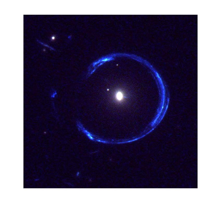
S. Schuldt et al.: The inner dark matter distribution of the Cosmic Horseshoe
construct a composite profile of baryons and dark matter. With its counter image, marked with a green dashed box in Fig. 1. For
such observations, one can very well fit the profile near the re- this counter image we have Gemini measurements (see Sec. 2.2)
gion of the Einstein ring, but the inner part cannot be well con- to yield a redshift of zs,r = 1.961 ± 0.001. A summary of various
strained due to the typical absence of lensing data in the inner re- properties about the Cosmic Horseshoe is given in Table 1.
gion. The presence of a radial arc, even though seldom observed
in galaxy-scale lenses, can help break the lensing degeneracies
and put constraints on the inner mass distribution. Another pos- The Cosmic Horseshoe
sibility is to combine lensing and dynamics, which is now a well
established probe to get for instance the density profile for early-
type galaxies (ETGs; e.g., Mortlock & Webster 2000; Treu &
Koopmans 2002, 2004; Gavazzi et al. 2007; Barnabè et al. 2009;
Auger et al. 2010; van de Ven et al. 2010; Barnabè et al. 2011;
Grillo et al. 2013).
In this paper, we present a detailed study of the inner mass
structure of the Cosmic Horseshoe lens through lensing and
combine these information with those coming from dynami-
cal modeling. The Cosmic Horseshoe, discovered by Belokurov
et al. (2007), is ideal for such a study: the deflector galaxy’s huge
amount of mass results in a spectacular and large Einstein ring,
and near the center of the lens exists a radial arc, which helps to G
constrain the mass distribution in the inner part of the Einstein
ring. To include the radial arc and our association for its counter
image in the models, we have spectroscopy measurements for O1
the counter image to get its redshift. O2
The outline of the paper is as follows. In Sec. 2 we introduce
the imaging and spectroscopic observations with their character-
istics and describe the data reduction and redshift measurement N
for the radial arc counter image. Then we revisit briefly in Sec. 3 O3
the multiple-lens-plane theory. In Sec. 4 we present our results
of the composite mass model of baryons and dark matter using 2 arcsec E
lensing-only, while in Sec. 5 we present the results of our mod-
els based on dynamics-only. In Sec. 6 we combine lensing and
dynamics and present our final models. Sec. 7 summarizes and
concludes our results.
Throughout this work, we assume a flat ΛCDM cosmol-
G
0.0055 0.087 0.17 0.25
G
0.33 0.41 0.49 0.57 0.66 0.74 0
ogy with Hubble constant H0 = 72 km s−1 Mpc−1 (Bonvin et al.
2017) and ΩM = 1 − ΩΛ = 0.32 whose values correspond to the
updated Planck data (Planck Collaboration et al. 2016). Unless
specified otherwise, each quoted parameter estimate is the me-
dian of its one-dimensional marginalized posterior probability
density function, and the quoted uncertainties show the 16th and
star 1 star 1
radial arc (color) radial arc (F475W)
84th percentiles (that is, the bounds of a 68% credible interval).
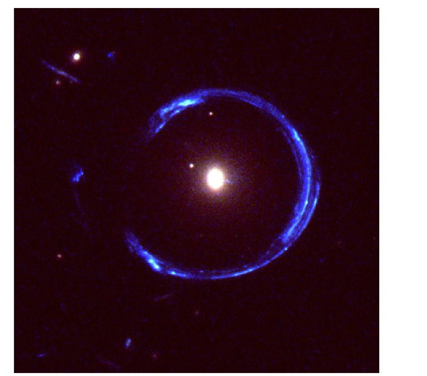
Fig. 1: Color image of the Cosmic Horseshoe obtained through a
combination of the F475W, F606W, and F814W filter images
2. The Cosmic Horseshoe (J1148+1930) from the HST WFC3. The size of this image is 2000 × 2000 .
The Cosmic Horseshoe, also known as SDSS J1148+1930, was One can see the ≈ 300◦ wide blue Einstein ring of the Cosmic
discovered by Belokurov et al. (2007) within the Sloan Digital Horseshoe. In addition, the Cosmic Horseshoe observation in-
Sky Survey (SDSS). A color image of this gravitational lensed cludes a radial arc which is marked with a green solid box. This
image is shown in Fig. 1. The center of the lens galaxy G, at a is shown in detail in in the bottom panel, in color (left) and
star 2 star 2
redshift of zd = 0.444, lies at (11h 48m 33 s .15; 19◦ 300 300 .5) of the from the F475W filter (right). We associate this radial arc to its
epoch J2000 (Belokurov et al. 2007). The tangential arc is a star- counter image, marked in the main figure with a dashed green
forming galaxy at redshift zs,t = 2.381 (Quider et al. 2009) which box and located around 800 on the east side of the lens galaxy G.
is strongly lensed into a nearly full Einstein ring (≈ 300◦ ), whose Both the radial arc and its counter image correspond to a source
radius is around 500 and thus one of the largest Einstein rings ob- at redshift zs,r = 1.961 (see Sec. 2.2). The three star-like objects
served up to now. This large size shows that this lens galaxy must in the field of view, which we include in our light model, are cir-
be very massive. A first estimate of the enclosed mass within the cled in yellow. The figures are oriented such that North is up and
Einstein ring is ≈ 5 × 10¹² M (Dye et al. 2008) and thus the lens East is left.
galaxy, a luminous red galaxy (LRG), is one of the most massive
galaxies ever observed. Apart from the nearly full Einstein ring
and the huge amount of mass within the Einstein ring, which
makes this observation already unique, the Cosmic Horseshoe 2.1. Hubble Space Telescope imaging
observations reveal a radial arc. This radial arc is in the west
of the lens, as marked in the green solid box in Fig. 1. We in- The data we analyse in this work come from the Hubble Space
clude this radial arc in our models as well as our association of Telescope (HST) Wide Field Camera 3 (WFC3) and can be
star 3
2S. Schuldt et al.: The inner dark matter distribution of the Cosmic Horseshoe
Table 1: Properties of the Cosmic Horseshoe (J1148+1930) 10
Hα
Flux (arbitrary units)
Component Properties Value 5
Lens Right ascensiona 11h 48m 33 s
0
Declinationa 19◦ 300 300 .5
a
Redshift, zd 0.444 −5
b
tangential arc source Redshift, zs,t 2.381
Star forming rateb ≈ 100 M yr−1
Ring Diameter a
10.200
Lengtha ≈ 300◦
Enclosed mass c,d
≈ 5 × 10¹² M
d
radial arc source Redshift, zs,r 1.961
References: 19200 19250 19300 19350 19400 19450 19500 19550
a Observed wavelength (Å)
Belokurov et al. (2007)
b
Quider et al. (2009)
c 15
Dye et al. (2008) [OIII] 5007Å
Flux (arbitrary units)
d
result presented in this paper
10
5
0
downloaded from the Mikulski Archive for Space Telescopes1 .
The observations with filters F475W, F606W, F814W, F110W, −5
and F160W were obtained in May 2010 (PI: Sahar Allam) and
the observations with the F275W filter in November 2011 (PI:
Anna Quider).
For the data reduction we use HST DrizzlePac2 . The size of
a pixel after reduction is 0.0400 for WFC3 UVIS (i.e. the F275W
F475W, F814W and F606W band) and 0.1300 for the WFC3 IR
(i.e. the F160W and F110W band), respectively. The software
includes a sky background subtraction. In our case the subtracted 14700 14750 14800 14850 14900 14950
background appears to be overestimated since many of the pixels Observed wavelength (Å)
have negative value, possibly due to the presence of a very bright
and saturated star in the lower-right corner of the WFC3 field of Fig. 2: Top (Bottom): 2d and 1d spectrum around the Hα
view (≈ 16000 ×16000 ). Since negative intensity is unphysical and ([OIII] 5007Å) emission line from the counter-image to the ra-
we fit the surface brightness of the pixels, we subtract the median dial arc, obtained from GNIRS observations. The 1D spectrum is
of an empty patch of sky that we pick to be around 2500 N-E to the extracted from a 5 pixel, corresponding to 0.7500 , aperture around
Cosmic Horseshoe from all pixels of the reduced F160W-band each line.The secondary peak redward of [OII] visible in the 1D
image. After our background correction, around 300 pixels (≈ spectrum is due to a cosmic ray that was not properly removed
1.3% of the full cutout) of the corrected image still have negative in the data reduction process.
values, which is consistent with the number given by background
noise fluctuations. We proceed in a similar way with the F475W
band, where the number of negative pixel is still high but in the
range of background fluctuations.
2.2. Spectroscopy: redshift of the counter image of radial arc
To align the images of the different filters we are using in
this paper, we model the light distribution of the star-like objects We obtained a spectrum of the counter-image to the radial arc us-
O2 and O3 (see Fig. 1) in the F475W band, masking out all the ing the Gemini Near-InfraRed Spectrograph (GNIRS; Elias et al.
remaining light components (such as arc, lens and object O1). 2006) on the Gemini North Telescope (Program ID: GN-2012B-
We do not include object O1 in the alignment since we do not Q-42, PI Sonnenfeld). We used GNIRS in cross-dispersed mode,
model the light distribution of the lens in this band and the lens with the 32 l/mm grating, the SXD cross-dispersing prism, short
has significant flux in the region of O1 that could affect the light blue camera (0.1500 /pix) and a 700 × 0.67500 slit. This configura-
distribution of O1. From this model and our lens light model tion allowed us to achieve continuous spectral coverage in the
in the F160W band, which we present in Sec. 4.2.1, we get the range 9, 000 − 25, 000Å with a spectral resolution R ∼ 900. We
coordinates of the centers of both objects in the two considered obtained 18 × 300s exposures, nodding along the slit with an
bands. Under the assumption these coordinates should match, ABBA template.
we are able to align the F475W and the F160W images.
We reduced the data using the Gemini IRAF package. We
identified two emission lines in the 2D spectrum, plotted in Fig.
1
http://archive.stsci.edu/hst/search.php 2: these are Hα and [OIII] 5007Å, at a redshift zs,r = 1.961 ±
2
DrizzlePac is a product of the Space Telescope Science Institute, 0.001. From here on, we take this to be the redshift of the radial
which is operated by AURA for NASA. arc and its counter-image.
3S. Schuldt et al.: The inner dark matter distribution of the Cosmic Horseshoe
3. Multi-plane Lensing We can then compute the average surface mass density with the
formula
In this work we employ multi-plane gravitational lensing, given
the presence of two sources at different redshifts (correspond- RR
Σ(R0 ) 2πR0 dR0
ing to the tangential and radial arcs, respectively). We therefore Σ(< R) = 0
. (9)
briefly revisit in this section the single plane and generalized πR2
multi-plane gravitational lens formalism. In the single plane for-
These general equations hold in the single plane case, but for the
malism a light ray of a background source is deflected by one
multi-plane case one defines similar, so-called effective, quanti-
single lens whereas, in the multi-plane case, the same light ray
ties. For calculating the effective convergence κeff one replaces
is deflected several times by different deflectors at different red-
in Eq. 6 the deflection angle α with the total deflection angle
shifts (e.g., Blandford & Narayan 1986; Schneider et al. 2006;
αtot from Eq. 2. In analogy to the case above one computes the
Gavazzi et al. 2008). The lens equation of the multi-plane lens
effective average surface mass density Σeff (< R), now using κeff
theory, which gives the relation between the angular position θ j
instead of κ. The consequence is that this quantity Σeff (< R) is
of a light ray in the j-th lens plane and the angular position in
the gradient of the total deflection angle αtot instead of a physi-
the j = 1 plane, which is the observed image plane, is given by
cal surface density.
j−1
X Dk j
θ j (θ1 ) = θ1 − α̂(θ k ) , (1)
k=1
Dj 4. Lens mass models
where θN = β corresponds to the source plane if N is the number Since the position of an observed gravitationally lensed image
of planes, θk is the image position on the k-th plane, α̂(θk ) is the depends on both baryonic and dark matter, one can use gravi-
deflection angle on the k-th plane, Dk j is the angular diameter tational lensing as a probe for the total mass, i.e. baryonic and
distance between the k-th and j-th plane, and D j is the angular dark matter together. We start with a model of the lensed source
diameter distance between us and the j-th plane. The total de- positions, i.e. surface brightness peaks in the observed Einstein
flection angle αtot is then the sum over all deflection angles on ring, with a single power-law plus external shear for the total
all planes mass. In addition to the main arc, which is the tangential arc,
this model includes the radial arc and its counter image and is
N−1
X DkN presented in Sec. 4.1. Based on this, we construct a composite
αtot = α̂(θk ) . (2) mass model to describe the total mass. To disentangle the visible
k=1
DN
(baryonic) matter from the dark matter, we model the lens light
In the case of N = 2 the general formula reduces to the well distribution (see Sec. 4.2.1) which is then scaled by a constant
known lens equation for the single plane formalism, namely mass-to-light ratio M/L, for the baryonic mass. Combining the
total mass and the baryonic mass, we construct in Sec. 4.2.2 a
Dds composite mass model of baryons and dark matter assuming a
β=θ− α̂(Dd θ) . (3) power-law (Barkana 1998), a NFW profile (Navarro, Frenk, &
Ds
White 1997), or a generalized NFW profile for the dark matter
Here the only lens is at θ = θ1 , the source at β = θ2 , α̂ is the (to- distribution. We use then a model based on the full HST images
tal) deflection angle, and Dds , Ds and Dd the distances between (Sec. 4.3) to refine our image positions (Sec. 4.4). In these mod-
deflector (lens) and source, observer and source, and observer els we always include the radial arc and our assumption for its
and deflector, respectively (e.g. Schneider et al. 2006). counter image. Only in the last section with the redefined image
The magnification µ is in the multi-plane formalism defined positions we treat explicitly models with and without the radial
in the same way as in the single plane formalism, namely arc as constraints. This would allow us to quantify the additional
constraint on the inner dark matter distribution of the Cosmic
1
µ= (4) Horseshoe from the radial arc, which is the primary goal of this
det A paper.
with the Jacobian matrix For the modeling, we use Glee (Gravitational Lens Efficient
Explorer), a gravitational lensing software developed by
∂β ∂θ N S. H. Suyu and A. Halkola (Suyu & Halkola 2010; Suyu et al.
A= = . (5)
∂θ ∂θ1 2012). This software contains several types of lens and light pro-
files and uses Bayesian analysis such as simulated annealing and
For the surface mass density Σ(R) one needs the convergence
Markov Chain Monte Carlo (MCMC) to infer the parameter val-
κ, sometimes also called the dimensionless surface mass density.
ues of the profiles. The software also employs the Emcee pack-
In the single-lens plane case, the convergence is
age developed by Foreman-Mackey et al. (2013) for sampling
∂α1 ∂α2 the model parameters.
2κ = + = ∇θ · α , (6)
∂θ1 ∂θ2
where α = (Dds /D s )α̂. This can then be multiplied with 4.1. Power-law model for total mass distribution
In this section, we consider a simple power-law model for the
c2 Ds
Σcrit = (7) total lens mass distribution, which has been shown by previ-
4πG Dd Dds ous studies to describe well the observed tangential arc (e.g.,
to derive Σ(R) using the definition of convergence Belokurov et al. 2007; Dye et al. 2008; Quider et al. 2009;
Bellagamba et al. 2017). This will allow us to compare our
Σ(R) model, that includes the radial arc, with previous models. We vi-
κ= . (8) sually identify and use as constraints six sets of multiple image
Σcrit
4S. Schuldt et al.: The inner dark matter distribution of the Cosmic Horseshoe
positions, where each set comes from a distinct source compo- 4.2.1. Lens light distribution for baryonic mass
nent. For modeling the lensed source positions we choose the
image of the F475W band, since one can distinguish better be- To disentangle the baryonic matter from the dark matter, we need
tween the different parts of the Einstein ring and since the arc a model of the lens light distribution. For this we mask out all
is bluer than the lens galaxy. This is an indicator that the lens flux from other components such as stars and the Einstein ring
galaxy is fainter and therefore one can better identify multiple in the image of the F160W filter. We then fit the parameters to
images in F475W. Here we use a singular power-law elliptical the observed intensity value by minimizing the χ2lens , which is
mass distribution (SPEMD; Barkana 1998) with slope γ0 = 2g+1 defined as
γ0 −1
for the lens (where the convergence κ(θ) ∝ θ ) with an ex- 2
Np
ternal shear. We infer the best-fit parameters of this model by X I obs sersic
j − PSF ⊗ I j
minimizing χ2lens = . (11)
j=1
σ2tot, j
pred 2
Npt
X θobs
j − θj Here Np is the number of pixels, σtot, j the total noise, i.e.
χ2 = (10)
j=1
σ2j background and Poisson noise (see below for details), of pixel
j, and ⊗ represents the convolution of the point spread func-
pred tion (PSF) and the predicted intensity. It is necessary to take
with Glee. Here Npt is the number of data points, θ j the pre- the convolution with the PSF into account due to telescope ef-
j the observed image position, with σ j the corre-
dicted and θobs fects. Here we use a normalized bright star ≈ 4000 S-W of the
sponding uncertainty of point j. Cosmic Horseshoe lens as the PSF. We subtract also from the
This model contains six sets of multiple images in addition PSF a constant to counterbalance the background coming from
to the radial arc and its counter image (see Fig. 6 with refined a very bright object in the field of view which scatters light over
identifications that will be described in Sec. 4.4). This model has the image.
a χ2 of 12.6 for the image positions and the best-fit parameter We approximate the background noise σbkgd as a constant
and median values with 1-σ uncertainties are given in Table 2. that is set to the standard deviation computed from an empty
The obtained marginalized and best-fit values for the total mass region. We also include the contribution of the astrophysical
model are in agreement with models from previous studies (e.g., Poisson noise (Hasinoff 2012), which is expressed as a count
Dye et al. 2008; Spiniello et al. 2011). rate for pixel i
√
σ0tot,i
!2 !2
Table 2: Best-fit and marginalized parameter values for the di ti di
σ2poisson,i = = = , (12)
model assuming a power-law profile plus external shear. ti ti ti
where ti is the exposure time, di the observed intensity of pixel
component parameter best-fit value marginalized value i (in e− -counts per second) and σ0tot,i is the total Poisson noise
x [00 ] 10.86 10.92+0.05
(labeled with an apostrophe as it is not a rate like σpoisson,i ). We
−0.05
include the contribution of the astrophysical Poisson noise only
y [00 ] 9.60 9.61+0.04
−0.04 if it is larger than the background noise. We sum the background
q 0.76 0.78+0.04
−0.04 noise and astrophysical noise in quadrature, such that σ2tot, j in
power-law θ [rad] 0.58 0.51+0.07
−0.08
Eq. (11) is
θE 8.06 7.6+0.5
−0.5
σ2tot, j = σ2bkgd, j + σ2poisson, j . (13)
rc [00 ] 0.01 0.29+0.3
−0.3
γ0 1.7 2.0+0.4
−0.2
Sersic
shear γext 0.08 0.07+0.02
−0.02
φext [rad] 3.5 3.2+0.2
−0.3
To describe the surface brightness of the Cosmic Horseshoe lens
galaxy, we use the commonly adopted Sersic profile (Sérsic
Note. The parameters x and y are centroid coordinates with respect to 1963), which is the generalization of the de Vaucouleurs law
the bottom-left corner of our cutout, q is the axis ratio, θ is the position (also called r1/4 profile, De Vaucouleurs 1948). For modeling the
angle measured counterclockwise from the x-axis, θE is the Einstein lens light distribution we choose the observation in the F160W
radius, rc is the core radius, γ0 is the slope, γext is the external shear band, since the lens is brighter in F160W than in the other bands,
magnitude, and φext is the external shear orientation. The constraints for and infrared bands trace better the stellar mass of the lens galaxy.
this model are the selected multiple image systems. The best-fit model
has an image position χ2 of 12.6. The best-fit model obtained by using two Sersic profiles
and two stellar profiles (in this model we include two star-
like objects, labelled object O1 and object O2 in Fig. 1) has
χ2 = 2.73 × 10⁴ (corresponding to a reduced χ2 of 1.74).
4.2. Components for composite mass model
Chameleon
Since the light deflection depends on both the baryonic and the
dark matter, we can construct a composite mass model. For the In addition to our lens light distribution model with the Sersic
baryonic component, we need a model of the lens light to scale it profile, we also model with another type of profile which mim-
by a mass-to-light ratio (Sec. 4.2.1). Since we do not have other ics the Sersic profile well and allows analytic computations of
information to infer the dark matter component, we fit to the data lensing quantities (e.g., Maller et al. 2000; Dutton et al. 2011;
using different types of mass profiles (Sec. 4.2.2). Suyu et al. 2014). It is often called chameleon and composed by
5S. Schuldt et al.: The inner dark matter distribution of the Cosmic Horseshoe
a difference of two isothermal profiles: 4.2.2. Dark matter halo mass distribution
In the previous section we have derived the baryonic compo-
L(x, y) = 1+q
L0
√ 1
nent by modeling the light distribution. To disentangle the bary-
L
x2 +y2 /q2L +4w2c /(1+qL )2 onic mass from the dark component, we model the dark mat-
ter distribution using three different profiles. At first we use
− √ 1 . (14) a NFW (Navarro et al. 1997) profile but, since newer simula-
x2 +y2 /q2L +4w2t /(1+qL )2 tions predict deviations from this simple profile, we present in
addition the best-fit mass model obtained assuming a power-
In this equation, qL is the axis ratio, and wt and wc are parameters
law profile (Barkana 1998, Singular Power-Law Elliptical Mass
of the profile with wt > wc to keep L > 0.
Distribution) (with parameters q as axis ratio, θE as Einstein ra-
By modeling with the chameleon profile we assume the same
dius, and rc as core radius) and a generalized version of the NFW
background noise as using the Sersic profile (see Sec. 4.2.1).
profile, given by
Since the model including two isothermal profile sets and two
stellar profiles for the two objects, as used above with the Sersic ρs
profile, has a χ2 of around two times the Sersic-χ2 , we add a third ρ(r) = γ 3−γg , (16)
× 1 + rrs
r g
chameleon profile and get a χ2 of 2.89 × 10⁴ which corresponds rs
to a reduced χ2 of 1.85. In this model we include also objects
O1, O2 and O3 (numbering follows Fig. 1), since we want to use where γg is the inner dark matter slope. The generalized NFW
the coordinates for the alignment of the two considered bands, profile reduces to the standard NFW profile in the case γg = 1.
F160W and F475W. We assume an axisymmetric lens mass distribution (axisym-
We will use both filters in the extended source modeling (see metric in 3 dimensions), and impose the projected orientation of
Sec. 4.3) while in the models using identified image positions the dark matter profile to be 0◦ or 90◦ rotated with respect to
we only use the F160W band for the lens light fitting. The pa- that of the projected light distribution. We find that the 90◦ ori-
rameter values of this best-fit model are used for the mass mod- entation gives a better χ2 , and thus the dark matter halo seems to
eling (given in Table 3) and the corresponding image is shown in be prolate, for an axisymmetric system that has its rotation axis
Fig. 3. The left image shows the observed intensity and the mid- along the minor axis of the projected light distribution. Since
dle the modeled intensity. In the right panel one can see the nor- strong lensing is only sensitive on scales of the Einstein radius,
malized residuals of this model in a range (−7σ, +7σ). The con- we assume four different values for the scale radius in the NFW
stant gray regions are the masked-out areas (containing lensed and gNFW profile, namely rs ≡ 18.1100 , 36.2200 , 90.5400 , and
arcs and neighbouring galaxies) in order to fit only to the flux of 181.0800 . These values correspond to 100 kpc, 200 kpc, 500 kpc,
the lens. Although there are significant image residuals visible in and 1000 kpc, respectively, for the lens redshift in the considered
the right panel, the typical baryonic mass residuals (correspond- cosmology. We include the mass of the radial arc source in the
ing to the light residuals scaled by M/L) would lead to a change model, using a singular isothermal sphere (SIS) profile, as this
in the deflection angle that is smaller than the image pixel size source galaxy’s mass will deflect the light coming from the back-
of 0.00 13 at the locations of the radial arc. ground tangential arc source. The center of this profile is set to
In Fig. 4 we show the contributions of the different com- the coordinates for the radial arc source which we obtained from
ponents, plotted along the x-axis of the cutout in units of solar the multiplane lensing, calculated by the weighted mean of the
luminosities for comparison of the contribution of the different mapped positions of the radial arc and its counter image on the
light profiles. To compare those components’ widths to that of redshift plane of the radial arc.
the PSF, in the same figure we show the latter (black dotted line)
scaled to the lens light of the central component (plotted in red). 4.3. Extended source modeling
To convert the fitted light distribution into the baryonic mass,
we assume at first a constant mass-to-light ratio. This means In the next stage of our composite mass model, we reconstruct
we scale all three light components by the same M/L value. the source surface brightness (SB) distribution and fit to the ob-
Additionally, we explore models with different M/L values for served lensed source light, i.e. the main arc and the radial arc
the different components, either two ratios with M/Lcentral = with its counter image. This will help us to refine our image posi-
M/Lmedium or M/Lmedium = M/Louter and the remaining differ- tions afterwards. For this, we start with the mass model obtained
ent, or with three different M/L values one for each component. in Sec. 4.2.2, which includes the lens light distribution described
These baryonic mass models are considered in the Sections 4.3 by the three chameleon profiles scaled with a constant mass-to-
and 4.4.1. Furthermore, since the width of the central compo- light ratio as baryonic mass and a power-law profile for the dark
nent, shown in red in Fig 4, is comparably to the PSF’s width, matter halo. We then allow the mass parameters to vary and,
and based on our modeling results in Section 4.4.1, we model in for a given set of mass parameter values, Glee reconstructs the
Section 6 this central component by a point mass with Einstein source SB on a grid of pixels (Suyu et al. 2006). This source is
radius described by then mapped back to the image plane to get the predicted arc. To
4GM infer the best-fit parameters, one optimizes with Glee the poste-
θE,point = (15) rior probability distribution which is proportional to the product
c 2 Dd of the likelihood and the prior of the lens mass parameters (we
(where the Einstein radius is defined here for a source at redshift refer to Suyu et al. (2006) and Suyu & Halkola (2010) for more
infinity), superseding the model that scales the central compo- details). The fitting of the SB distribution has
nent with an M/L. Here G is the gravitational constant, M the
point mass, c the speed of light, and Dd the distance to the de- χ2SB = (d − dpred )T CD−1 (d − dpred ) , (17)
flector. For the remaining two components (blue and green in
Fig. 4) we assume either one or two different mass-to-light ra- where d = dlens + darc is the intensity values d j of pixel j written
tios to scale the light to a mass. as a vector with length Nd , the number of image pixels, and CD
6S. Schuldt et al.: The inner dark matter distribution of the Cosmic Horseshoe
-15 -8.5 -2 4.5 (a) observed
11 18 24 30 37 44 -15 50 -8.5 -2 4.5 11 (b) model
18 24 30 37 44 -7 50 -5.6 -4.2 (c) normalized residuals
-2.8 -1.4 0.0068 1.4 2.8 4.2 5.6 7
Fig. 3: The best-fit model for the lens light distribution. The left image shows the observation of the Cosmic Horseshoe in the
F160W-band, whereas the central panel shows the predicted light distribution. This model includes three chameleon profiles (see
Eq. 14) and two PSF and one de Vaucouleurs profiles for the three objects. The right image shows, in a range between −7 σ
and +7 σ, the normalised residuals of this model. The constant gray regions are the masked-out areas (containing lensed arcs and
neighboring galaxies) in order to fit only to the flux of the lens. The figures are oriented such that North is up and East is left.
1010 component 1 and model the radial arc and its counter image separately due
component 2 to their different redshift from the tangential arc. This is done
component 3 only in the F475W filter. The light component parameter values
109 PSF
of this model, with a χ2SB of 7.2 × 10⁴ for the F160W filter and
3.1 × 10⁵ for the F475W filter (the corresponding reduced χ2SB
108
for the total model is 1.37), are presented in Table 3. In the same
L [M ]
table we also give the median values with 1-σ uncertainty. The
107 corresponding images of the best-fit model are presented in Fig.
5. In the top row one sees the images of the F160W band, in the
106 middle row the images of the tangential arc and lens light in the
F475W band, and in the bottom row the images of the radial arc
105 in the F475W band, respectively. The images are ordered, for
each row from left to right, as follows: the first image shows the
104 observed data, the second the predicted, the third image shows
10.0 7.5 5.0 2.5 0.0 2.5 5.0 7.5 10.0 the normalized residuals and the fourth image displays the re-
r [arcsec] constructed source. Despite visible residuals in the reconstruc-
tion, some of which are due to finite source pixel size, we are
Fig. 4: Different components of the chameleon profiles shown reproducing the global features of the tangential arcs (compare
in units of solar luminosity, respectively in red (“inner”), blue panels a to b, and e to f), to allow us to refine our multiple image
(“medium”), and green (“outer” component). The total light ob- positions.
served from the Cosmic Horseshoe lens galaxy in the HST filter
We also model the Cosmic Horseshoe observation with
F160W is described by the sum of all three components. For
source SB reconstruction assuming the NFW or gNFW for the
comparison of the width of the components the scaled PSF is
dark matter halo mass. The fits give for the NFW based model a
plotted with a black dotted line.
χ2SB of 3.76 × 10⁵ (corresponding to a reduced χ2SB = 1.37) and
very similar values for the gNFW model. From this, it seems that
the gNFW fits almost as well as the NFW profile. Compared
is the image covariance matrix. In the pixellated source SB re- with the power-law extended source model, the χ2 is slightly
construction, we impose curvature form of regularization on the higher, but still comparable. The images reproduce the observa-
source SB pixels (Suyu et al. 2006). tions comparably well assuming the power-law profile, as shown
Since we use the observed intensity of the arc to constrain in Fig. 5.
our mass model and the F475W band has the brightest arc rela-
tive to the lens light, we include the F475W band in addition to
the F160W which is used for the lens light model. For simplic- 4.4. Image position modeling
ity we assume the same structural parameters of the lens light
profiles in the two bands (such as axis ratio q, center, and orien- Finally, we refine multiple image systems using the extended
tation θ) and model only the amplitude of the three chameleon surface brightness modeling results of the last section. This time
profiles and of the three objects included. Explicitly, we model we find, similarly to what was done in Sec 4.1, eight sets of mul-
the lens galaxy’s light in both filters and reconstruct the observed tiple images systems, in addition to the radial arc and its counter
intensity of the Einstein ring in both. We also need to specify image.
7S. Schuldt et al.: The inner dark matter distribution of the Cosmic Horseshoe
-5 -2.5 -0.015 2.5
(a) observed
5 7.5 10 12 15 -5 18 -2.5 20 -0.015 2.5
(b) predicted
5 7.5 10 12 15 -7 18 -5.6 20 -4.2
(c) normalized residuals
-2.8 -1.4 0.0068 1.4 2.8 4.2 -0.26 5.6 -0.00147 (d) source reconstruction
0.26 0.52 0.78 1 1.3 1.6 1.8 2.1 2.3
-0.08 -0.052 -0.024 0.004
(e) observed
0.032 0.06 0.088 0.12 0.14 -0.080.17 -0.0520.2 -0.024 0.004
(f) predicted
0.032 0.06 0.088 0.12 0.14 -7 0.17 -5.6 0.2 -4.2
(g) normalized residuals
-2.8 -1.4 0.0068 1.4 2.8 4.2 -0.0675.6 -0.026 7
(h) source reconstruction
0.016 0.058 0.1 0.14 0.18 0.23 0.27 0.31 0.35
-0.0020 0.0022 0.0064 0.0106
(i) observed
0.0148 0.0190 0.0232 0.0274 0.0316 -0.0020
0.0358 0.0022
0.0400 0.0064 0.0106
(j) predicted
0.0148 0.0190 0.0232 0.0274 0.0316 -70.0358 -5.60.0400 -4.2
(k) normalized residuals
-2.8 -1.4 0.0068 1.4 2.8 4.2 -0.045.6 -0.028 7 -0.016
(l) source reconstruction
-0.0037 0.0083 0.02 0.032 0.044 0.057 0.069 0.081
Fig. 5: Images for the best-fit model which includes the source surface brightness reconstruction. In the top row one sees the images
of the F160W band, and in the middle (tangential arc with lens) and bottom (radial arc) rows the images of the F475W band,
respectively. To separate the radial arc and the tangential arc is needed since they lie at a different redshift. The images are ordered
from left to right as follows: observed data, predicted model, normalized residuals in a range from −7σ to +7σ and the reconstructed
source SB on a grid of pixels.
4.4.1. Three chameleon profiles the radial arc and its counter image. Here we have to remove the
SIS profile which we adopt for the radial arc source mass. With
If we assume a constant M/L for all three chameleon profiles this model we get a best-fit χ2 of 18.87 which corresponds to a
to scale the light to the baryonic mass, our model predicts the reduced χ2 of 1.18.
positions very well, with a χ2 of 20.23, which corresponds to a
reduced χ2 of 1.07 (in equation 10) . Here we use the best-fit
model obtained in Sec. 4.3, which adopts the power-law profile, Similarly as before, we test how well we can fit the same
now with core radius set to 10−4 , for the dark matter distribution. multiple image systems, i.e. these eight sets for the tangential
This is done since the value is always very small and we want arc and the radial arc with its counter image as shown in Fig.
to focus on constraining the slope. Another reason is that we 6, with our model by assuming a NFW or gNFW dark matter
need to fix one parameter for our dynamics-only model which distribution. It turns out that our model based on the NFW profile
is explained more in Sec. 6. The model with the selected multi- gives a χ2 of 35.48 (reduced χ2 = 1.87) whereas the model based
ple image systems is shown in Fig. 6. The figure shows also the on the gNFW profile gives a χ2 of 35.19 (reduced χ2 = 1.96).
critical curves and caustics for both redshifts, zs,r = 1.961 and This means that we do not fit the refined multiple image systems
zs,t = 2.381, as well as the predicted image positions from Glee. with the NFW or gNFW dark matter distribution as well as with
The filled squares and circles correspond to the model source po- the power-law. We see a big difference in χ2 compared to the
sition (which is the magnification-weighted mean of the mapped models where we exclude the radial arc and its counter image.
source position of each image). Explicitly, without radial arc are the χ2 values 25.44 (reduced
To compare how much constraints we get from the radial arc, χ2 = 1.59) and 25.40 (reduced χ2 = 1.70) for the NFW and
we treat also a model based on these image positions excluding gNFW profile, respectively.
8S. Schuldt et al.: The inner dark matter distribution of the Cosmic Horseshoe
Table 3: Best-fit and marginalized parameter values for the lens light component of the mass model obtained by reconstructing the
source surface brightness.
Chameleon 1 (lens) Chameleon 2 (lens) Chameleon 3 (lens)
parameter best-fit value marginalized value best-fit value marginalized best-fit value marginalized
x[00 ] 11.00 − 11.00 − 11.00 −
00
y[ ] 9.67 − 9.67 − 9.67 −
qL 0.62 0.64+0.02
−0.03 1.00 +0.00
1.00−0.01 1.00 1.00+0.00
−0.01
θ[rad] 1.52 − 1.52 − 1.52 −
L0 (F160W) 46.67 − 3.50 − 8.56 −
wc 0.08 0.07+0.01
−0.01 1.95 +0.06
2.04−0.07 0.18 0.20+0.03
−0.02
wt 0.18 0.18+0.01
−0.01 6.99 +0.03
7.01−0.06 1.24 1.31+0.02
−0.03
L0 (F475W) 0.11 0.11+0.01
−0.01 0.027 0.029+0.001
−0.001 0.010 0.010+0.001
−0.002
Note. This model includes three chameleon profiles (see Eq. (14)) for the F160W filter and additionally the same profiles with the same structural
parameters for the F475W band. We fix the amplitudes of the F160W band since we are multiplying them with the mass-to-light ratio (variable
parameter) in constructing the baryonic mass component.
While the power-law halo model fits well to the image posi- on dynamics-only (e.g., Yıldırım et al. 2016; Nguyen 2017;
tions, it yields a M/L of around 0.4 M /L that is unphysically Yıldırım et al. 2017; Wang et al. 2018).
low. On the other hand, the NFW and gNFW with a common For the dynamical modeling we use a software which was
M/L for all three light components cannot fit well to the image further developed by Akın Yıldırım (Yıldırım et al. in prep.) and
positions, particularly those of the radial arc. Since newer publi- which is based on the code from Michele Cappellari (Cappellari
cations (e.g., Samurović 2016; Sonnenfeld et al. 2018; Bernardi & Copin 2003; Cappellari 2008). For an overview of the Jeans
et al. 2018) predict variations in the stellar mass-to-light ra- ansatz and the considered parameterization, the Multi-Gaussian-
tio of massive galaxies, we treat our model of the refined im- Expansion (MGE) method, see Appendix 8. We infer the best
age position models with different mass-to-light ratios for each fit parameters again using Emcee as already done for the lensing
chameleon profile. Different ratios result in a similar effect as a part.
radial-varying ratio. We treat this variation of different M/L for
all our models, that means both with and without radial arc as
well as for all three different dark matter profiles NFW, gNFW 5.1. Lens stellar kinematic data
and power-law. This will be considered further in Sec. 6.
Following the discovery of the famous Cosmic Horseshoe by
Belokurov et al. (2007), several follow-up observations were
4.4.2. Central point mass with constant M/L of extended done. In particular, Spiniello et al. (2011) obtained long slit kine-
chameleon profiles matic data for the lens galaxy G in March 2010. This was part of
their X-Shooter program (PI: Koopmans). The observations cov-
Since (1) we get a very small M/L for the central component
ered a wavelength range from 300 Å to 25000 Å simultaneously
(compare red line in Fig. 4) in the previous model, (2) this com-
with a slit centered on the galaxy, a length of 1100 and a width of
ponent is very peaky that the width is smaller as the PSF width,
0.00 7.
and (3) the Cosmic Horseshoe galaxy is known to be radio ac-
tive, we infer that the central component is a luminous point To spatially resolve the kinematic data, they defined seven
component like an AGN. Thus we cannot assume an M/L for apertures along the slit and summed up the signal within each
it to scale to the baryonic matter. Therefore we treat also mod- aperture. The size of each aperture was chosen to be bigger than
els where we assume a point mass instead of the central light the seeing of ≈ 0.00 6, such that independent kinematic measure-
component. The mass range is restricted to be between 108 M ment for each aperture were obtained. These data are listed in
and 1010 M as these are the known limits of black hole masses Table 4, together with the uncertainties. The obtained weighted
(e.g., Thomas et al. 2016; Rantala et al. 2018). For the two other, average value of the velocity dispersion is 344 ± 25 km s−1 . This
extended chameleon profiles, we assume a M/L to scale them is within the uncertainty of the measurements. Due to the small
to the baryonic mass. Under this assumption we are able to re- number of available data and the huge errors we will consider
produce a good, physical meaningful model for all three adopted the symmetrized values and uncertainties as given in Table 4.
dark matter profiles. Since our final model will also include the For further details on the measurement process or the data of
kinematic information of the lens galaxy, we will discuss details the stellar lens kinematics see Spiniello et al. (2011).
only for this model in Section 6.
5.2. Dynamics-only modeling
5. Kinematics & Dynamics
Before we combine all available data to constrain maximally the
In Sec. 4 we construct a composite mass model of the Cosmic mass of the Cosmic Horseshoe lens galaxy, we model the stel-
Horseshoe lens galaxy using lensing alone. In this section lar kinematic data alone. We start from the best-fit model from
we present the kinematic data of the Cosmic Horseshoe lens lensing, and include the parameters anisotropy β and inclination
galaxy taken from Spiniello et al. (2011) and a model based i. Since we have only seven data points (see Table 4), we can
9S. Schuldt et al.: The inner dark matter distribution of the Cosmic Horseshoe
Table 4: Stellar kinematic data of the Cosmic Horseshoe lens galaxy.
Aperture distance [00 ] v [kms−1 ] σ [km s−1 ] vrm s [km s−1 ] vrms, sym [km s−1 ]
−2.16 −100 ± 100 350 ± 100 364 ± 101 406 ± 101
−1.36 −80 ± 100 311 ± 76 321 ± 78 340 ± 89
−0.64 −9 ± 25 341 ± 26 341 ± 27 353 ± 26
0.00 0 ± 12 332 ± 16 332 ± 16 332 ± 16
+0.64 62 ± 18 360 ± 25 365 ± 25 353 ± 26
+1.36 77 ± 80 350 ± 100 358 ± 100 340 ± 89
+2.16 180 ± 100 410 ± 100 448 ± 101 406 ± 101
Note. We give the distance along the slit measured with respect to the center, the corresponding rotation v (Spiniello et al. 2011), the velocity
dispersion σ (Spiniello et al. 2011), the second velocity moments vrms obtained through Eq. (28), and the symmetrized values vrms, sym . The
√
uncertainties δvrms is calculated through the formula δvrms = v2 δv2 + σ2 δσ2 /vrms . The last row are the considered values in this section.
20 vary at most six parameters. Thus we set the core radius rc of
the power-law, which turned out to be very small in our lensing
models, to 10−4 . For a correct comparison to the refined lens-
ing models (see Sec. 4.4) we fix the core radius there too. For
dynamics we will only adopt power-law and NFW dark matter
15 distribution, i.e. no longer the generalization of the NFW profile.
The reason is the small improvement compared to the NFW pro-
file. One further reason is that otherwise we have to fix one pa-
rameter to vary fewer parameters than the available data points.
y [arcsec]
In other words, for considering the generalized NFW profile we
12
10 have to fix one parameter such that the number of free parame-
ters is smaller than the number of data points. In analogy to the
case of the power-law profile where we fix the core radius, we
9 1011 11 12 13 would set for the generalized NFW profile the slope γg ≡ 1. This
5
x [arcsec] would result in the NFW profile.
y [arcsec]
The power-law dark matter distribution gives a dynamics-
10 only best-fit model with χ2 = 0.25. The reason why our model
has a χ2 much smaller than 1 is due to the big uncertainties. The
0 data points are shown in Fig. 7 (blue) with our dynamics-only
0 5 10 15 20 model assuming power-law (solid) or NFW (dashed) dark mat-
9 x [arcsec] ter distribution. Since we can easily fit to these seven data points
in the given range, we treat the same model also with forecasted
Fig. 6: Best-fit model of the lensed source positions of the 5% uncertainties for every measurement. The obtained best-fit
Cosmic Horseshoe, which are identified using our best-fit mass dynamics-only model has a χ2 of 4.95, which is clearly much
model with source SB reconstruction. This model assumes a
8 higher than for the full error. The best-fit parameter and median
power-law 9 profile 10 11 matter 12
for the dark 13 It is ob-
distribution. values with 1-σ uncertainty are given in Table 5 for the model
tained using, as constraints,xeight
[arcsec]
multiple image systems for assuming the actual measured errors. As expected, most param-
the Einstein ring (circles) and the radial arc and its counter im- eters are within the 1-σ range and the mass-to-light ratio is in a
age (squares). We mark the predicted image positions with a good range. The relatively large errors on the parameters are due
cross. One can see that all predicted images are very close to the to the small number of data points we use as constraints.
selected ones. The blue lines correspond to the critical curves
(solid) and caustics (dashed) computed for the redshift of the ra-
dial arc, i.e. zs,r = 1.961, and the red line to the critical curves For the NFW dark matter distribution we fit comparably well
(solid) and caustics (dashed) computed for the redshift of the as with the power-law model (χ2 = 0.25 compared to χ2 = 0.26),
tangential arc, i.e. zs,t = 2.381. The lens position is marked when using the full kinematic uncertainty, while the χ2 is slightly
with a blue star. The small additional red features near the ra- higher for the reduced (forecasted 5%) uncertainty on the kine-
dial arc source position, shown in the lower left corner in detail, matic data (χ2 = 4.95 compared to χ2 = 5.61). Comparing
and on the right hand side are probably due the presence of ra- power-law and the NFW, we do not find a remarkable difference,
dial arc source, i.e. as a result of multi-plane lensing. Indeed, apart for the radius, which appears to be lower in the NFW fore-
we can see that these features do not appear in the single-plane casted case. This, however, is in agreement with the higher χ2
case (blue line). The filled squares and circles correspond to the of the NFW since the predicted vrms values are in both versions,
weighted mean positions of the predicted source position, which power-law and NFW profile, lower than the measurement. For
are shown in more detail in the zoom in the upper/lower left cor- a further detailed analysis based on dynamics-only spatially, re-
ner. The figure is oriented such that North is up and East is left. solved kinematic measurements would be helpful.
10S. Schuldt et al.: The inner dark matter distribution of the Cosmic Horseshoe
Table 5: Best-fit parameter values for our model based on the tary of these two approaches. However, in our particular lens
power-law dark matter distribution with dynamics-only. system, we also use the radial arc as lensing constraints in the
inner regions.
Although using the HST surface brightness observations
component parameter best-fit value marginalized
would provide more lensing constraints, we consider here only
kinematics β 0.10 0.01+0.2
−0.3 the refined image positions presented in Sec. 4.4. The reason for
+0.2 this choice is that we would otherwise overwhelm the 7 data
i 0.1 0.1−0.2
dark matter q 0.82 0.83+0.2
points from dynamics with more than 105 surface brightness
−0.09
+0.5
pixel from the images. The data points coming from the iden-
(power-law) θE [00 ] 2.3 2.4−0.4 tified image positions are still higher, but at the same order of
00 −4
rc [ ] ≡ 10 − magnitude. Moreover, with this method we are able to weight
γ 0
1.20 1.36+0.4 the contribution of the radial arc and its counter image more.
−0.2
baryonic matter M/L [M /L ] 1.8 +0.4
1.6−0.6 When we combine dynamics and lensing, we consider again
models with and without radial arc, each adopting power-law or
Note. The parameters are the anisotropy β, the inclination i, the axis NFW dark matter distribution, and all four versions with the full
ratio q, the strength θE , the core radius rc , and the slope γ0 . In the last uncertainty of the kinematic data as well as with 5% as a fore-
row we give the mass-to-light ratio for the baryonic component. Since cast. Additionally, we treat all models with one single M/L ratio
we have only seven data points with huge uncertainties and vary six as well as with different M/L ratios as already done for lensing-
parameters in this model, we get also a large range of parameter values only (see Sec. 4.2.1 for details). Based on the same arguments
within 1-σ. The corresponding χ2 is 0.25. Note that we do not obtain as for the lensing-only, we treat also models by replacing the
any constraints on the anisotropy or inclination, given the assumption PSF-like central component (shown in red in Fig. 4) by a point
of a prior range of β ∈ [−0.3, +0.3] and i ∈ [0, +0.3].
mass.
500 data 6.1. Three chameleon mass profiles
power-law dark matter
450
NFW dark matter By combining lensing and dynamics we consider different com-
posite mass model. As first, we use the lens light, which is com-
posed by three chameleon profiles as obtained in Sec. 4.2.1,
scaled by a constant mass-to-light ratio as baryonic component.
vrms [km s 1]
400
Under this assumption, the best-fit has, when using a power-law
dark matter mass distribution, a χ2 of 25.08, and, when using
350 a NFW dark matter distribution, a χ2 of 71.54. The χ2 values
reveal that the NFW is not as good at describing the observa-
tion as the power-law profile. However, assuming a power-law
300 dark matter distribution, the M/L value for scaling all three light
components is around 0.1M /L . This is unphysically low and
250 results in a very high the dark matter fraction.
2 1 0 1 2 The next step to model the baryonic component is to allow
r [arcsec] different mass-to-light ratios for the different light components
shown in Fig. 4. This allows us to fit remarkably better with the
Fig. 7: Values for the second velocity moments vrms obtained by NFW profile, while we do not get much improvement adopting a
adopting the power-law dark matter distribution (solid gray) or power-law dark matter distribution. However, this method does
NFW (dashed blue) for dynamics-only. In brown are shown the not allow us to obtain meaningful models, as the central com-
measured data points with the full error bars. ponent needs an unphysically low M/L. Therefore, we infer that
we cannot assume a mass-to-light ratio for the central compo-
nent, irrespective of the dark matter distribution.
6. Dynamical and lensing modeling
After modeling the inner mass distribution of the Cosmic 6.2. Point mass and two chameleon mass profiles
Horseshoe lens galaxy based on lensing-only (Sec. 4) and
dynamics-only (Sec. 5), we now combine both approaches. In As noted in Sec. 4.4.2, the central component is probably asso-
the last years huge effort has been spent to combine lensing and ciated with an AGN, since its light profile width is similar to the
dynamics for strongly lensed observations to get a more robust width of the PSF (see Fig. 4) and its M/L was very low from the
mass model (e.g., Treu & Koopmans 2002, 2004; Mortlock & previous model in Sec. 6.1. Thus, assuming a mass-to-light ratio
Webster 2000; Gavazzi et al. 2007; Barnabè et al. 2009; Auger for this component would not be physically meaningful and we
et al. 2010; Barnabè et al. 2011; Sonnenfeld et al. 2012; Grillo supersede it by a point mass in the range of a black hole mass.
et al. 2013; Lyskova et al. 2018). Since strong lensing has nor- From our previous models and from the fact that the lens galaxy
mally the constraints at the Einstein radius r ≈ θE , which is in is very massive, we expect this point mass to be comparable to
our case ≈ 500 , and kinematic measurements are normally in that of a supermassive black hole. For the two other light compo-
the central region around the effective radius (here r . 200 ), nents we still assume the two fitted chameleon profiles scaled by
one combine information at different radii with these two ap- a M/L, either the same M/L for both components, or a different
proaches. This will result in a better constrained model and one M/L for each component. Moreover, we test the effect of relax-
might break parameter degeneracies thanks to the complemen- ing the scale parameter rs of the NFW profile. It turn out to be
11You can also read