October 2020 No: 1309 - Decoding India's low Covid-19 case fatality rate
←
→
Page content transcription
If your browser does not render page correctly, please read the page content below
Decoding India’s low Covid-19 case fatality rate

                    Minu Philip , Debraj Ray & S. Subramanian

                    (This paper also appears as CAGE Discussion paper 516)

          October 2020                                                   No: 1309

                Warwick Economics Research Papers

ISSN 2059-4283 (online)
ISSN 0083-7350 (print)
Decoding India’s Low Covid-19 Case Fatality Rate†

                          Minu Philip, Debraj Ray and S. Subramanian‡
                                               September 2020

Abstract. India’s case fatality rate (CFR) under covid-19 is strikingly low, with a current level
of around 1.7%. The world average rate is far higher. Several observers have noted that
this difference is at least partly due to India’s younger age distribution. We use age-specific
fatality rates from 17 comparison countries, coupled with India’s distribution of covid-19
cases, to “predict" India’s CFR. In most cases, those predictions yield even lower numbers,
suggesting that India’s CFR is, if anything, too high rather than too low. We supplement the
analysis with a decomposition exercise, and we additionally account for time lags between
case incidence and death for a more relevant perspective under a growing pandemic. Our
exercise underscores the importance of careful measurement and interpretation of the data,
and emphasizes the dangers of a misplaced complacency that could arise from an exclusive
concern with aggregate statistics such as the CFR.

1. Introduction

As of September 10, 2020, India has 4.5 million confirmed cases of covid-19, with a death toll
of over 76,000. Figure 1 plots the case fatality rate [CFR] in India, compared to the world (Panel
A) and to selected countries (Panel B). Over the initial duration of this epidemic, India has
hovered around a CFR of 3% or more, with a steady downward trend to around 1.7%. The
world rate is far higher, trending down from a peak of over 7% to a current number around
3%. Several economically advanced countries are far higher still. Panel B of Figure 1 compares
India to a number of other countries — these comparisons will recur throughout the paper.
India is at or near the bottom of the case fatality heap. The end-August fatality rate of 1.8%
compares favorably with countries such as the Netherlands (8.9%), Italy (13.2%), and Spain
(6.3%).

Of course, CFRs are not to be confused with infection fatality rates, the latter being the true
measure of mortality from the disease. But covid-19 infection rates are not known anywhere
in the world, and in India they are currently the subject of considerable debate.1 Therefore, at
least for assessing trends and comparisons, we must currently make do with CFRs. And it is

    † We  thank Dean Spears for useful comments, and Vrinda Anand for helpful assistance. Ray acknowledges
research support from the National Science Foundation under Grant no. SES-1851758.
    ‡ Philip: New York University, minu.philip@nyu.edu, Ray: New York University and University of Warwick,

debraj.ray@nyu.edu. Subramanian: Independent researcher, ssubramanianecon@gmail.com.
    1 Bhramar Mukherjee, in private communication, suggests a nationwide under-reporting factor of the order of

15-25, implying a current infected population of 30-50 million. See Bhattacharyya et al. (2020) for more details on
the calculation of the under-reporting factor for India.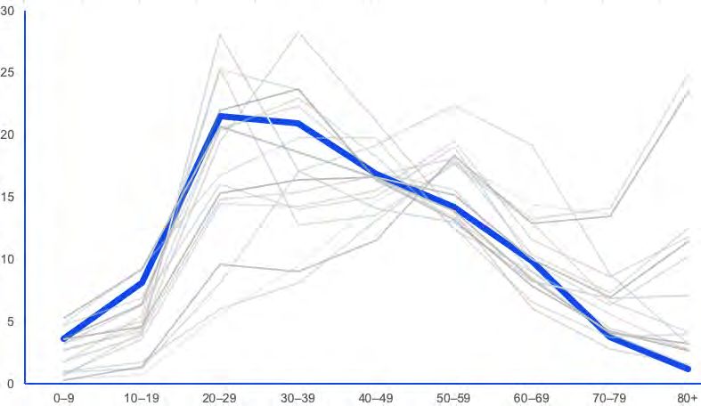
(a) India and World                                       (b) India and Others

  Figure 1. Case Fatality Rates for India and Selected Countries over Apr 01 - Sept 10, 2020. Source.
  Roser et al. (2020)

not a bad measure at all for this purpose, provided that the absolute numbers are not interpreted
literally,2 and are only used to make comparisons across countries and time; that too with a
great deal of care.

Certainly, India’s seeming robustness under this measure (compared to other countries) has
not gone unnoticed. Government spokespersons have attributed it to “early identification and
clinical management of cases." Prime Minister Modi, in a national address on July 26, 2020,
while correctly emphasizing the need to “remain vigilant," observed that “India’s covid-19
recovery rate is better than others. Our fatality rate is much less than most other countries."3

To move from a low CFR to an unqualified commendation of deliberate policy-induced
recovery from the disease might (to put it mildly) overlook certain crucial aspects of
demographic detail. That the age distribution within a country will influence the CFR
for covid-19 is widely known, with “younger countries" exhibiting lower CFRs simply on
account of lower death rates among younger age groups. Many observers have pointed to
the Indian age structure as a possible confounding variable in interpreting the aggregate CFR;
see, for instance, Ray and Subramanian (2020) and Mukhopadhyay (June 11, 2020) for India
in particular, and Dudel et al. (2020) for other countries.4
     2 There are many reasons why the absolute values of CFRs have no obvious and natural meaning, some of

which will play an unavoidable role in this paper.
     3 The Hindustan Times, July 26, 2020; https://www.hindustantimes.com/india-news/pm-narendra-modi-s-67th-

mann-ki-baat-address-to-nation-highlights/story-bXhnWiU1WElwNLFp0mpWRJ.html.
     4 There are, of course, several other reasons for the CFR to vary across countries. Countries with higher

testing rates will generally have lower CFRs — spotting more cases at an earlier and presumably milder stage.
Moreover, CFRs will tend to trend down over time within the same country, as its testing improves. Actually,
India is pretty low on the world testing scale as measured by per-capita tests, so this logic suggests that its CFR
                                                        2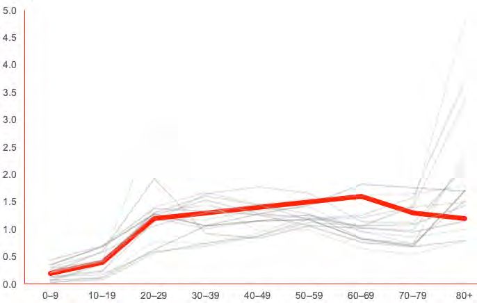
We take this observation as a starting point, but seek a more precise quantitative comparison
between India and other countries. Sections 2–4 deal with alternative approaches to this
question, so as to provide an overall assessment of India’s CFR.

One way of adjusting for age-distribution in a relatively young country is to ask what would
happen to that country’s overall CFR if it experienced age-specific CFRs similar to those in
countries in which older cohorts account for a larger share of the population. In Section 2, we
do this for India using a set of selected comparison countries and regions: the same set that
appears in Figure 1. A majority of these countries underpredict Indian rates in this exercise, even
though their overall CFRs are far higher than that of India.

With detailed age-specific data for both India and comparison countries, one can additionally
decompose the differences in CFRs for a sharper description of how the distribution of
cases and deaths by age affect aggregate mortality statistics. The method is different from
that in Section 2, in that it precisely separates the difference in CFR into two effects: one
corresponding to case distribution (an “incidence effect"), and the other to age-specific fatality
rates (the “fatality effect"). Our approach is based on Shorrocks (2013) and Kitagawa (1955),
and corresponds closely to that taken by Dudel et al. (2020) to explain the observed cross-
country variation in CFRs of selected countries; see Section 3 for details. We find that India’s
low CFR, while seemingly comparable (at least currently) to countries such as South Korea,
masks significant differences in age-specific incidence and mortality burdens from those of
South Korea, and only appears to be of comparable magnitude by a serendipitous opposition
of these factors in the process of aggregation.

The preceding analysis is based on the presumption that current deaths divided by current
cases is a good measure of case fatality. But this is problematic because there is a time-lag
between the onset of infection and the date of death. Verity et al. (2020) report a mean
duration of around 18 days from infection to death (conditional on death). It is unclear when
such cases would be registered as “confirmed" — that would depend on testing times — but
in any event, cumulative deaths should be related to cumulative cases at some anterior date.
This suggests that the contemporaneous CFR is an inaccurate reflection of the actual case
mortality rate. A better approximation is the number of covid deaths on a particular date
divided by the number of covid cases at some relevant anterior date. With cases mounting
over time, the contemporaneous CFR will understate case fatality relative to this “lagged CFR."
That would be true for all countries, but the extent of underestimation would be different for
different countries because of inter-country variation in the rate of growth of cases. Section
4 undertakes a comparison of India with selected countries, while exploring the difference
between contemporaneous and lagged CFRs. Using a three-week lag, the results are quite

should be higher, not lower. There are other ancillary issues, such as obvious caveats associated with using data
from multiple sources, such as definitional differences in what constitutes a ”covid-19 death.” There is also the
question of under-reporting (Pundir 2020; Thapar 2020; Chatterjee 2020), though this will affect both numerator
and denominator in the CFR.
                                                       3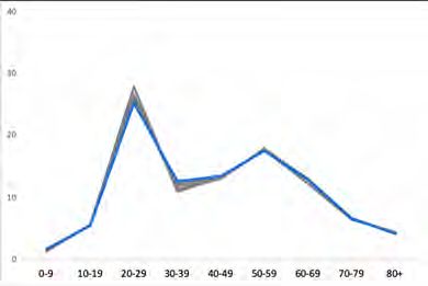
remarkable. For the overwhelming majority of countries that we consider, India’s advantage
in age-specific incidence is more than nullified by the higher age-specific mortality burdens.

We note that in making these comparisons, we have simply ignored the enormous problem of
undercounting of covid-19 deaths. Of course this matters, but even the reported deaths suffice
to make our point.

To summarize: there are two potential sources of difficulty in simply accepting the case fatality
rate, as it is usually reported, as a reliable indicator of cross-country comparison. (This is quite
separate from the inadequacy of CFRs as a true measure of covid-19 fatality, a well-known
issue that we do not address here.) The first has to do with the failure of the measure to reflect
the precise age-distribution of cases and deaths in each particular situation. The second has to
do with the strong possibility that a lagged CFR is a more dependable indicator of case fatality
than the customary contemporaneous CFR. Correcting for these complications, as we shall
see, leads to a picture of India’s health-related capability in dealing with the covid-19 epidemic
which is altogether less flattering than what might otherwise appear to be the case. This is
one more instance of the general proposition that careful measurement can make a difference
to our assessment of actual country performance in the matter of human development and
capabilities.

2. Predicting Indian Mortality from Age-Specific CFRs of Other Countries

To fix some elementary ideas and notation: let f c be the overall CFR in any country c, f jc the
CFR in age-group j, and let wcj be the proportion of all cases in age-group j. Then, for any
country,
                                             M
                                             X
                                        fc =    wcj f jc ,
                                                j=1

where M is the number of age groups. Begin by looking at India’s weight distribution {wIj },
which marks the incidence of the disease across different age groups. Figure 2 displays
information on the population distribution by age, the weight distribution by age, and the
impact ratios, which we define to be wcj /ncj , where ncj is the population share in age group j for
country c. These objects are displayed in Table 1.

The first exercise that we conduct is to “predict" case fatality rates for India using age-specific
data from a set of comparison countries, but using weights from the case distribution pertaining
to India. The idea is to approximate how India would perform if it had the age-specific case
fatality rates of these comparison countries. As it happens, our set of comparisons is perforce
limited because information on cases and deaths by age is not easy to come by and needs
to be extracted from individual country dashboards. Many countries do not provide those
data or (as in the case of India) do so infrequently and irregularly via Ministerial decree. As
of August 4, the Wikipedia website https://en.wikipedia.org/wiki/Coronavirus_disease_2019 lists 22
                                                 4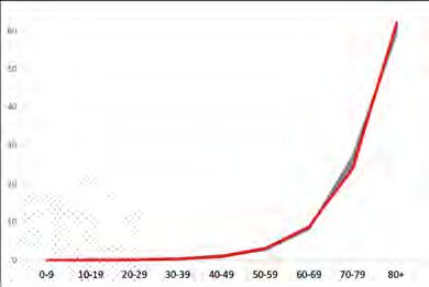
Age Group
0-9 10-19 20-29 30-39 40-49 50-59 60-69 70-79 80+
Case % [1] 3.6 8.1 21.5 21.0 16.8 14.2 9.9 3.8 1.2
Pop % [2] 17.0 18.3 17.4 15.6 12.3 9.3 6.3 2.8 1.0
Impact [1/2] 0.2 0.4 1.2 1.3 1.4 1.5 1.6 1.3 1.2
Table 1. Case incidence, population distribution and impact ratios for India. Impact ratios show
how different age-groups are affected relative to their population share. Sources. Case distribution
from ICMR COVID Study Group et al. (2020) and population distribution from UN World Population
Prospects (United Nations, Department of Economic and Social Affairs, Population Division 2019)
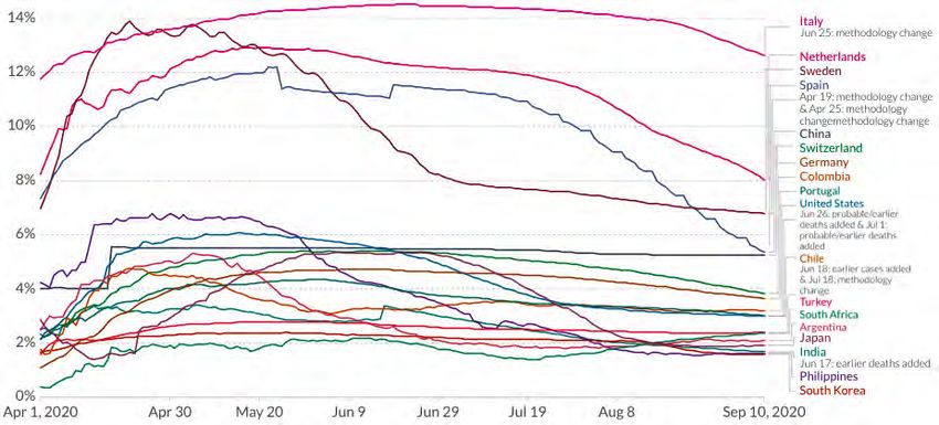
(a) Cases by Age (b) Impact Ratios by Age
Figure 2. Distribution of Cases and Impact Ratios by Age for India and Selected Countries. For list
of countries see text. Panel A shows the percentage of cases in each age group by country, Panel
B plots the impact ratio by age, by country. A ratio greater than 1 indicates that the age group
in question has been disproportionately hit relative to its population share. In each panel, India
is shown in bold and comparison countries are as listed in Table 2. Sources. Case Distribution
(see Table 7) and Population Distribution from UN World Population Prospects (United Nations,
Department of Economic and Social Affairs, Population Division (2019)).
countries with age-specific, country-level mortality rates, of which we use fifteen: Argentina,
Chile, China, Colombia, Germany (Bavaria), Italy, Japan, the Netherlands, the Philippines,
Portugal, South Africa, South Korea, Spain, Sweden, and Switzerland. We add the State of
California and Turkey for a total of seventeen comparison “countries.".5
Figure 2A shows the percentage of covid-19 cases by age group for India and the comparison
countries, with the Indian line depicted in boldface. Relative to our comparison list — with the
exception of other developing countries such as South Africa — India is demographically a
5 The remaining seven countries are Australia, Canada, Denmark, Finland, Israel, Mexico and Norway.
Including them does not affect the analysis but lengthens the tables without much added insight.
5
very young country indeed. The burden of the Indian case distribution by age therefore
sharply falls upon the younger age groups: the corresponding lines for several of the
comparison countries are shifted to the right.

Panel B plots the impact ratio — the ratio of case incidence to population percentage by
age, by country. A ratio greater than 1 indicates that the age group in question has been
disproportionately hit relative to population size. India is shown in bold. For all countries,
the impact ratios are smaller than one for the youngest age group, which is only to be
expected: after all, the very youngest are relatively isolated from widespread, anonymous
social interaction. But among working adult groups and relative to the comparison countries,
India stands out in having a large impact ratio. These middle-aged and older working
groups are not only those excessively represented in overall population (Panel B), they are
also disproportionately more affected by covid-19. In contrast, the Indian impact ratio is only
slightly above 1 for the oldest age groups, while for many of the comparison countries, that
impact ratio spikes upward quite dramatically. Taken together, these two features (population
distribution and the distribution of impact ratios) create a substantial skew, at least in the
measured incidence of covid-19, among the younger age groups.6 For the exact distributions
of cases and deaths by age for our comparison countries, see Table 7 in the Appendix.

These distributions come from a variety of dates for different countries. Unfortunately, for
countries for which age-based mortality data is taken from data visualization dashboards,
previous information often disappears from the visualization once updated, so that we
typically have access to age-specific data at one date, that of the latest update. But there
are exceptions. These exceptions suggest that barring the initial phases of the pandemic,
the distribution of cases and deaths across ages appears to be reasonably stable. We explore
this stability in Appendix 5.3. That is not true of the age-specific mortality rates, which do
change significantly over time. But the point is that the latter changes because there has
been significant movement in the case-fatality rate over time, and not because the relative
dispersion of cases or deaths has been changing. This feature will be exploited in the analysis
below.

We can use India’s case distribution information, along with the CFR patterns from com-
parison countries, to “predict" India’s CFR were it to be driven by the age-specific rates in
those countries, coupled with India’s case distribution across ages (which mirrors Indian
demographics). Table 2, which significantly extends Table 3 in Ray and Subramanian (2020),
carries out these predictive exercises. Specifically, country c’s prediction for India can be
written as
                                                 M
                                                 X
                                        f ˆc,I =   wIj f jc ,
                                                       j=1

   6 It
      is possible that relative to the comparison countries, the old remain at home in India during their illness,
and covid deaths as well as cases are disproportionately undercounted among them.
                                                        6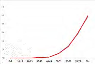
Predicted CFR at Various Dates
                                CFR
                               Jul 30 June 20 July 10 July 30       Aug 20 Sept 10
                India                     3.28        2.72   2.21      1.90      1.68
                China        5.34         2.85        2.84   2.78      2.73      2.73
                S. Korea     2.10         1.08        1.03   1.00      0.90      0.76
                Japan        3.09         2.29        2.03   1.32      0.84      0.82
                Philippines  2.30         4.07        2.61   2.35      1.65      1.67
                Netherlands 11.45         2.46        2.42   2.29      1.91      1.61
                Italy       14.24         3.18        3.15   3.11      3.03      2.76
                Spain        9.96         2.44        2.37   2.11      1.62      1.14
                Bavaria      5.16         1.94        1.92   1.87      1.76      1.57
                Sweden       7.54         2.45        2.10   2.03      1.90      1.83
                Switzerland  4.90         1.34        1.29   1.22      1.11      0.96
                S. Africa    1.59         2.47        1.85   1.88      2.46      2.79
                Chile        2.64         1.35        1.67   2.02      2.08      2.10
                Colombia     3.42         2.89        3.14   3.06      2.84      2.87
                Argentina    1.85         2.02        1.60   1.51      1.63      1.71
                Turkey       2.47         2.11        2.01   1.97      1.90      1.91
                Portugal     3.41         1.22        1.11   1.04      1.00      0.92
                California   1.83         2.36        1.69   1.38      1.37      1.42

  Table 2. Predicted Indian CFRs. Numbers in the first row report India’s CFR for different dates.
  Subsequent rows report counterfactual CFR for India, predicted using age-specific CFRs of the
  respective comparison country and India’s case distribution (Table 1). Under-predicting countries
  are highlighted in blue. Country-specific CFRs, as of July 30, are reported in red for comparison.
  Sources. Case and Death Distributions (Table 7) combined with CFRs from Roser et al. (2020) to
  calculate age-specific CFRs.

where the weights are the Indian distribution of cases across the population.

India’s latest CFR numbers stand at around 1.7%, but as Figure 1 also reveals, India’s CFR has
been around 3% for much of the period since the start of the pandemic, hitting 3.4% on June
17 as an adjustment of past deaths was made in the database; then falling slowly. Depending
on the dates for counterfactual prediction — we use five — we have different rates for India,
which are described in Table 2. Countries that (age-adjusted with Indian weights) predict a
lower CFR — relative to India’s actual aggregate CFR — are shown in blue. Note that some
country-level observations are mixed over time.

The adjusted CFRs in Table 2 are quite remarkable, given that the actual CFRs for many of
these countries far exceed those of India (Figure 1, Panel B). Countries such as the Netherlands
or Spain have a CFR well in excess of 9%. Yet, once adjusted for the Indian case distribution,
it becomes clear that India is no longer an outlier. While the reader is invited to go through
the comparisons, we single out South Korea here, because age-unadjusted, the two CFRs are
comparable as of July 30, 2020. And yet, once we adjust for differences in the demographic
                                                  7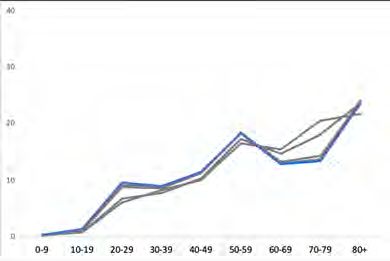
distribution, the South Korean rates translate into an aggregate CFR of merely 0.76%, far lower
than India’s CFR of around 1.68%.
There are over-predictors. Among them are Colombia, China, Turkey and Italy, the last of
which comes as a bit of a (relative) surprise.7 Compared to these countries, India’s performance
does not look as bad. We will revisit Table 2 with our study of lagged fatalities in Section
4. But even at this stage, it appears safe to dismiss as exaggeration the assertion that India’s
“fatality rate is much less than most other countries."
3. Decomposing Inter-Country Differences in Case Fatality Rates
3.1. A Decomposition. For a meaningful comparison of CFRs across two countries, we
decompose the difference in CFRs into what may be called a fatality effect and a case-incidence
effect. Let I stand for India, our country of interest, and let C be any comparison country. We
“decompose" this difference into two terms, as follows:
1 c 1
fc − fI = ( f − f I) + ( f c − f I)
2 2
M M M M
1 c X I c X c I I 1 c X I c X c I
= (f − wj fj + wj fj − f ) + ( f + wj fj − wj fj − f I)
2 2
j=1 j=1 j=1 j=1
M M
1 X
1
X
= (wcj − wIj )( f jc + f jI ) + ( (wcj + wIj )( f jc − f jI )
2 2
j=1 j=1
M M
1 X 1 X
= ∆w j ( f jc + f jI ) + (wcj + wIj )∆ f j , (1)
2 2
j=1 j=1
where ∆w j = wcj − wIj , and ∆ f j = f jc − f jI . This decomposition is an instance of the Shapley
procedure described by Shorrocks (2013), based on Shapley’s 1953 formulation of his celebrated
“value" as a solution to allocation problems within a cooperative game. In the specific context
of our paper, this approach coincides with a procedure advanced by Kitagawa (1955), which
seeks to factorize the “difference between two rates" into its “component" parts (Preston,
Heuveline, and Guillot 2001). Dudel et al. (2020) apply this procedure to differences in
case fatality rates, as we do here. Note that this is an exact decomposition, that is, the
relative contributions of the factors driving the change under examination add up to exactly
100% (without leaving behind any hard-to-interpret residual effects, such as the so-called
“interaction" effect in “standard" decompositions).
7 The Italian comparison exhibits some contrast to Mukhopadhyay’s June 11, 2020 analysis. He undertakes
a similar exercise as in Table 2 using Italian data, and reports that: “[B]y multiplying Italy’s age-specific CFR
. . . to the age-specific number of cases in India, [we find that] [t]he estimated numbers of deaths that should have
occurred, if the age-specific death rates of Italy were to prevail in India, is 535. The official number of deaths
in India as of April 30 was actually twice that number, at 1074." We go some way towards a resolution of this
difference in Section 4, though the disparity is still puzzling.
8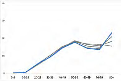
The first component in the decomposition (1) is what we may call the incidence effect. It
quantifies the difference in CFRs that would arise solely due to age-specific differences in
case incidence rates under the hypothetical scenario that the countries share the average of
their age-specific CFRs. This number will typically be positive if the comparison country is
older, because older age groups are weighted by higher fatality rates and the comparison
country will have more of such groups. The second component, which we call the fatality
effect, quantifies the difference in CFRs that would arise solely due to differences in age-specific
CFRs, in the hypothetical scenario that the countries share the average of their age-specific
infection rates. This number would be negative if India’s age-based fatality rate is higher
than the corresponding age-based fatality rate for the comparison country, for most, if not all
age groups. The fatality effect is closely related to the analysis in Table 2, where we “predict"
Indian CFR using India’s case distribution, except that here we use as weights the average of the
case distribution for India and the comparison country in question. Because the economically
advanced countries among the latter group are more likely to have an older population, this
tempers the prediction somewhat, and we expect milder effects compared to Table 2.

3.2. Decomposing India’s CFR. The decomposition formula relies on more data than in Section
2; specifically, on the distribution of deaths by age for India, a statistic released sporadically
by the Union Health Ministry and in age brackets that are both coarse and frustratingly non-
comparable with those used for our comparison countries. The latest numbers are from a
July 8 Press Release, with incidence for six age brackets. To maintain comparability, we’ve
split these brackets into the nine brackets used so far, drawing on additional data with an
interpolation procedure described in Appendix 5.2; see Table 3.

                                                     Age Group
                     0-9 10-19 20-29 30-39 40-49 50-59 60-69 70-79 80+
          Cases (%)  3.6   8.1 21.5 21.0 16.8 14.2       9.9   3.8 1.2
          Deaths (%) 0.8   0.9   2.4   5.5 13.5 24.0 30.4 15.9 6.7

  Table 3. Case and Death Distribution by Age for India. Sources. Case distribution from ICMR
  COVID Study Group et al. (2020) and death distribution interpolated using Indian Ministry of
  Health Press Release, July 08, 2020 (details in Appendix 5.2).

Armed with the information here and invoking similar data for the comparison countries,
we can set equation (1) to work. Table 4 studies three dates over which the Indian CFR
has progressively fallen (along with those of the comparison countries). For each of these
dates and each comparison country, we report the CFR of the country, which — barring a
few cases — significantly exceeds those of India. The decomposition exercise then breaks up
the difference between the Indian and comparison CFR into incidence and fatality effects, as
described in (1). The CFR difference is the sum (accounting for positive and negative values)
of the incidence and fatality effects.
                                                 9
June 20 July 30 Sept 10
Country CFR Diff IE FE CFR Diff IE FE CFR Diff IE FE
India 3.28 0.00 - - 2.21 0.00 - - 1.68 0.00 - -
China 5.49 2.21 2.52 -0.31 5.34 3.13 2.09 1.04 5.25 3.57 1.88 1.69
South Korea 2.26 -1.02 1.24 -2.26 2.10 -0.11 0.99 -1.10 1.59 -0.09 0.75 -0.84
Japan 5.35 2.07 2.14 -0.07 3.09 0.88 1.29 -0.41 1.92 0.24 0.86 -0.62
Philippines 3.97 0.69 -0.08 0.78 2.30 0.09 -0.05 0.14 1.63 -0.05 -0.04 -0.02
Netherlands 12.30 9.02 7.83 1.19 11.45 9.24 6.54 2.70 8.04 6.36 4.71 1.65
Italy 14.52 11.24 8.78 2.46 14.24 12.03 7.65 4.37 12.63 10.95 6.53 4.42
Spain 11.52 8.24 7.54 0.70 9.97 7.76 5.95 1.81 5.36 3.68 3.65 0.03
Bavaria 5.37 2.09 2.82 -0.73 5.16 2.95 2.39 0.56 4.35 2.67 1.96 0.71
Sweden 9.12 5.84 4.74 1.10 7.54 5.33 3.71 1.63 6.80 5.12 3.21 1.91
Switzerland 5.37 2.09 3.53 -1.43 4.90 2.69 2.86 -0.16 3.84 2.16 2.21 -0.06
South Africa 2.09 -1.19 -0.35 -0.84 1.59 -0.62 -0.25 -0.36 2.36 0.68 -0.30 0.98
Chile** 1.77 -1.51 0.41 -1.92 2.64 0.43 0.44 -0.01 2.74 1.06 0.42 0.64
Colombia 3.23 -0.05 0.22 -0.27 3.42 1.21 0.22 1.00 3.21 1.53 0.20 1.33
Argentina 2.48 -0.80 0.31 -1.12 1.85 -0.36 0.23 -0.59 2.09 0.41 0.24 0.18
Turkey 2.65 -0.63 0.47 -1.10 2.47 0.26 0.39 -0.13 2.40 0.72 0.35 0.37
Portugal 3.97 0.69 2.57 -1.88 3.41 1.20 1.99 -0.79 3.00 1.32 1.66 -0.33
California 3.12 -0.16 0.51 -0.66 1.83 -0.38 0.31 -0.69 1.87 0.19 0.29 -0.10
Table 4. CFR-Difference Decomposition For India and Comparison Countries. Sources. Distri-
bution of cases and deaths from Tables 3 and 7. These, along with overall CFRs from Roser et
al. (2020), are combined and applied to the decomposition formula (1) to obtain Incidence Effects
(IE) and Fatality Effects (FE).
Once again let’s single out South Korea, given that its CFR on July 30 (2.1%) is comparable with
that of India (2.2%). This comparability now appears clearly as the coincidental cancellation
of two opposing forces. The incidence effect is positive, which isn’t surprising given that
South Korea has an older population. The fatality-weighted distribution of cases generates a
higher fatality for South Korea on that score. But the fatality effect is negative — that is, the
case-weighted distribution of fatalities generates a larger number for India. The two effects
cancel, leaving them with comparable CFRs on the aggregate. The higher age-specific fatality
rate, as indicated by the negative fatality effect, is suggestive of a relatively lower level of
robustness of health in India, or a relatively lower level of robustness of treatment facilities,
or both. If India and South Korea shared their age-specific CFRs, their average, South Korea’s
aggregate CFR would be higher than India’s by close to one percentage point, a huge difference
relative to their baseline CFRs. Alternatively, with the same case distribution, South Korea’s
CFR would be lower by slightly more than one percentage point, owing to its low age-specific
CFRs.
The near-equivalence in the two CFRs is therefore a result of aggregation. The fatality effect
goes against a favorable welfare interpretation for India. But India’s particular pattern of the
age-distribution of Covid-19 incidence masks that negative effect. The same pattern recurs
for a number of other comparison countries, especially in the earlier months. To see this in
a bit more detail, consider the data for September 10. Of the 17 comparison countries, 6 are
10ones for which the IE and the FE have opposing signs, and in all but one of these cases (S.
Africa), the IE is positive and the FE negative. Of the remaining 11 cases, it is only in the
case of the Philippines that both effects are negative; in 8 of the other 10 cases (that is, barring
Chile and Colombia), both effects are positive, with the IE dominating the FE. In a majority
of cases, therefore, it is the differential age-distribution of covid cases that comes to India’s
rescue. Later, when we consider lagged CFRs (Table 6, these patterns acquire even greater
clarity.
This decomposition analysis goes beyond our earlier comparisons in Table 2, in that it also
includes the counterfactual when the CFRs are the same but case incidence isn’t. Here, India’s
“advantage" of higher case incidence among the young is not by virtue of its demographic
characteristics alone. A quick recall of the population shares and case shares in Table 1, along
with Panel B of Figure 2, reminds us that the caseload for the working-age population in
India is higher than its population share. In contrast to most other countries with the highest
impact ratio reserved for the oldest age group, it is the impact ratio for the middle-aged and
older working population that is relatively high in India. While this helps attenuate India’s
CFR, it is certainly not desirable otherwise. Why that population is disproportionately affected
requires an evaluation of exposure, prevalence of co-morbidities, or lifestyle choices such as
smoking, etc., which is beyond the scope of the present exercise.
All in all, the recipe for a low aggregate CFR looks quite simple to implement: pick either
an endowment of low age-specific CFRs, or a case distribution skewed towards low-CFR age
groups. India’s demographic structure generates an abundant supply of the second ingredient,
amplified by its high impact ratios for working-age groups. (The same is true of South Africa,
another young country.) In contrast, India appears to be lacking in the first ingredient: low
age-specific CFRs.
Comparisons such as those between India and South Korea are not intended to verify the easily
accessed fact that India has fared poorly in relation to a country which is an obvious outlier.
Such comparisons would then add up to no more than an essentially trite exercise. Rather,
the objective, at a general level, is to drive home the point that social indicators such as the
aggregate CFR are essentially outcome-indicators, and that in certain cases, similar outcomes
(as for India and South Korea) can display widely differing underlying processes that lead
up to these outcomes. Similar observations have been made by Anderson and Ray (2010)
and Jayaraj and Subramanian (2009) about the sex-ratio of a population, and by Kanbur and
Mukherjee (2007) about poverty indices. This general point reinforces the specific desirability
of guarding against misplaced complacency (or panic, as the case may be) that could arise
from an exclusive concern with an aggregate statistic such as the CFR.
114. Growing Epidemics and Lagged Case Fatality Rates
When a SARS-CoV-2 infection ends in death, the mean duration from symptoms to death is
around 2.5 weeks; see, for instance, Verity et al. (2020), who report a mean duration of around
18 days.8 It is unclear when such cases would be registered as “confirmed" before the death
occurs — that would depend on when testing occurs after the onset of symptoms — but it is
likely that the cumulative deaths at any date should be related to cumulative cases at some
anterior date, and not cumulative contemporaneous cases. Call this measure of case fatality
the lagged case fatality rate, or LCFR.
Using case counts from January 30, 2020 to May 14, 2020, Mohanty et al. (2020) find that the
14-day LCFR for India is 8.01%, more than twice the contemporaneous CFR of 3.40% on May
14, 2020. But it is no surprise to learn that in societies with growing incidence (or expansion of
testing), LCFR would significantly exceed CFR. That doesn’t require us to calculate anything.
A more interesting question emerges when we make comparisons across countries. Every
LCFR would exceed its contemporaneous counterpart. The question is: by how much? It is
easy to see that ceteris paribus, a country with a faster growth rate of confirmed cases would
exhibit a higher ratio of LCFR to CFR. A bit more formally, if we denote the x-day growth
rate of cases in country c by gc , where x is a number that we would need to settle upon, then
lagged fatality φc is connected to contemporaneous fatality f c by the obvious identity:
φc = f c [1 + gc ].
4.1. The Prediction Exercise of Section 2 Revisited, with Lagged CFR. We revisit two exercises with
lagged case fatality rates. The first is the prediction exercise from Table 2. That is, we use the
same set of comparison countries to predict the case fatality rate for India using India’s age
distribution coupled with the age-specific fatality rates for those countries. But we now do so
using lagged fatality rates. The following qualifications and remarks should be noted.
First, we’d like to use age-specific growth rates to achieve the correction, but this is data we do
not have, so we apply the same growth rate in cases to all age groups within a country. Second,
the growth rate — and consequently the predictions — will vary with the lag. Therefore, while
we report 21-day lags, we explore a 14-day alternative in Appendix 5.4. Third, the choice of
calendar date will matter, as it will affect not just the values of India’s case fatality rate, but
also the rate of growth of cases. Therefore we conduct three exercises: for June 20, July 30 and
Sept 10. As in Table 2, we hold fixed the distribution of cases and deaths across ages. (We again
refer the reader to Appendix 5.3 for the intertemporal stability of these distributions.) The age-
specific lagged CFRs are generated from aggregate fatality rates applied to these distributions,
and then used to make the Indian predictions. Finally, we reiterate that the specific values of
the LCFRs, while potentially of interest, are problematic to interpret. We know they will go
8 Based on a study of Chinese data by Yang et al. (2020), Wilson et al. (2020) conclude that “. . . a median of 13
days passed from pneumonia confirmation to death. . . "
12Predicted CFR for Different Date-Lag Combinations
June 20 July 30 Sept 10
Country CFR* 0 -14 -21 0 -14 -21 0 -14 -21
India 3.28 5.47 7.45 2.21 3.61 4.56 1.68 2.27 2.65
China 5.34 2.85 2.86 2.87 2.78 2.84 2.85 2.73 2.74 2.75
South Korea 2.10 1.08 1.14 1.17 1.00 1.05 1.08 0.76 0.88 1.01
Japan 3.09 2.29 2.38 2.42 1.32 1.88 2.11 0.82 0.93 1.03
Philippines 2.30 4.07 5.61 6.96 2.35 3.42 3.99 1.67 2.02 2.35
Netherlands 11.45 2.46 2.58 2.64 2.29 2.40 2.42 1.61 1.83 1.93
Italy 14.24 3.18 3.22 3.26 3.11 3.16 3.17 2.76 2.96 3.05
Spain 9.96 2.44 2.49 2.51 2.11 2.33 2.38 1.14 1.47 1.67
Bavaria 5.16 1.94 1.96 1.98 1.87 1.91 1.93 1.57 1.70 1.77
Sweden 7.54 2.45 3.27 3.74 2.03 2.11 2.16 1.83 1.88 1.91
Switzerland 4.90 1.34 1.35 1.36 1.22 1.28 1.31 0.96 1.07 1.12
South Africa 1.59 2.47 4.98 7.40 1.88 2.85 3.95 2.79 2.91 3.01
Chile 2.64 1.35 2.56 3.46 2.02 2.21 2.34 2.10 2.23 2.30
Colombia 3.42 2.89 4.99 6.85 3.06 5.12 6.57 2.87 3.44 3.93
Argentina 1.85 2.02 3.81 5.19 1.51 2.45 3.14 1.71 2.38 2.79
Turkey 2.47 2.11 2.32 2.41 1.97 2.09 2.16 1.91 2.08 2.15
Portugal 3.41 1.22 1.38 1.46 1.04 1.11 1.18 0.92 1.01 1.04
California 1.83 2.36 3.20 3.76 1.38 1.87 2.25 1.42 1.54 1.63
Table 5. Predicted Indian Lagged CFRs. Numbers in the first row report Indian LCFR for different
dates and lags (14, 21 day). Subsequent rows record predictions from comparison countries.
Under-predicting countries are highlighted in blue. *Country specific CFRs, as of July 30, are
reported in red for comparison. Sources. Case and Death Distributions (Table 7) combined with
case and death counts from Roser et al. (2020).
up with the lag, but their absolute magnitudes could reflect either changes in the progression
of the epidemic, or the intensity of testing. Rather, all we do is explore what this does to the
under- or over-prediction of India’s correspondingly lagged rate.
Table 5 reports the results. Lagged CFRs are generally sizably larger than contemporaneous
CFRs. The 21-day growth in cases in India was between 60–80%, which leads to higher
(and probably more accurate) estimates of case fatalities; these are recorded in the first row
of the table, along with the unlagged CFRs for easy comparison. The predicted rates from
comparison countries are recorded in the rows below. For some countries like South Korea,
Spain and Switzerland, the resulting changes are minimal, because there is a near-cessation
of growth in new cases during this period. But more generally, there is a significant increase
in under-prediction once the differential case growth is taken into account. For instance, Italy
now switches from being an over-predictor of India’s case fatality rate to being an under-
predictor in most cases. The point is that Italian cases have grown slower than Indian cases
during this time period, so India’s effective case fatality rate is significantly higher than the
rates in Table 2. The same switch also occurs for China at the earlier dates, and even at the
13latest date on record here, China remains comparable to India. The one country that appears
to be doing distinctly worse is Colombia, which is also experiencing rapid growth in cases,
and — at the later dates — is an over-predictor in both Tables 2 and 5.
June 20 July 30 Sept 10
Country LCFR Diff IE FE LCFR Diff IE FE LCFR Diff IE FE
India 7.45 0.00 - - 4.56 0.00 - - 2.65 0.00 - -
China 5.51 -1.94 4.06 -6.00 5.48 0.92 2.99 -2.06 5.29 2.64 2.24 0.40
S. Korea 2.45 -5.00 2.12 -7.13 2.26 -2.30 1.50 -3.80 2.12 -0.53 1.08 -1.61
Japan 5.66 -1.79 3.00 -4.79 4.92 0.36 2.25 -1.89 2.40 -0.25 1.18 -1.42
Philippines 6.79 -0.66 -0.16 -0.49 3.90 -0.66 -0.10 -0.56 2.29 -0.36 -0.06 -0.30
Netherlands 13.18 5.73 11.90 -6.16 12.10 7.54 8.89 -1.35 9.68 7.03 6.22 0.81
Italy 14.88 7.43 12.88 -5.45 14.51 9.95 9.99 -0.04 13.94 11.29 7.95 3.34
Spain 11.84 4.39 11.49 -7.10 11.24 6.68 8.60 -1.92 7.86 5.21 5.52 -0.31
Bavaria 5.48 -1.97 4.27 -6.24 5.35 0.79 3.25 -2.46 4.89 2.24 2.45 -0.21
Sweden 13.90 6.45 8.29 -1.84 8.04 3.48 4.90 -1.42 7.11 4.46 3.74 0.72
Switzerland 5.45 -2.00 5.48 -7.47 5.25 0.69 4.07 -3.37 4.49 1.84 2.90 -1.06
S. Africa 6.26 -1.19 -0.94 -0.25 3.34 -1.22 -0.53 -0.69 2.54 -0.11 -0.36 0.26
Chile** 4.52 -2.93 0.98 -3.92 3.06 -1.50 0.64 -2.13 3.00 0.35 0.51 -0.16
Colombia 7.66 0.21 0.53 -0.31 7.35 2.79 0.46 2.33 4.39 1.74 0.28 1.47
Argentina 6.36 -1.09 0.78 -1.87 3.84 -0.72 0.47 -1.19 3.42 0.77 0.38 0.39
Turkey 3.03 -4.42 0.77 -5.20 2.71 -1.85 0.56 -2.41 2.70 0.05 0.44 -0.39
Portugal 4.78 -2.67 4.38 -7.05 3.85 -0.71 3.00 -3.71 3.38 0.73 2.14 -1.40
California 4.97 -2.48 0.90 -3.38 2.97 -1.59 0.54 -2.13 2.15 -0.50 0.37 -0.86
Table 6. 21 day LCFR-Difference Decomposition For India and Comparison Countries. Sources.
Distribution of cases and deaths from Tables 3 and 7. These, along with total case and death
counts from Roser et al. (2020) are combined and applied to the decomposition formula (1) to
obtain Incidence Effects (IE) and Fatality Effects (FE).
4.2. The Decomposition Exercise of Section 3 Revisited, with Lagged CFR. Lagged CFRs can also
be taken to the decomposition exercise of Section 3. We do so in Table 6. The structure is
exactly the same as in Table 5. We study three dates — June 20, July 30 and Sept 10. This
time we construct all case fatality rates using a 21 day lag, the idea being that deaths at day t
are related to infection at day t − 18 or thereabouts, and allowing for an additional “detection
lag" of four days. (The findings are robust to different lags; see Table 8 in the Appendix for an
example using 14-day lags).
The first column of numbers in this table lists lagged CFR by country, and the second column
records the raw difference between the comparison country and India. Negative numbers
highlighted in blue indicate that the comparison country is “doing better" than India, either in
the CFR itself or in terms of the fatality effect (or both). Compared to Table 5, India’s aggregate
LCFR now edges closer to the comparison countries just on account of the lag alone. This
raw difference is broken up into an incidence and fatality effect, just as in in Table 2. Now
there is a larger set of fatality effects that are negative, suggesting that once lagged fatalities
are introduced, the average of age-specific fatalities — with weights equal to the average
14incidence of cases across India and the comparison country — is even less likely to be in
India’s favor.
5. Summary and Discussion
The Indian case fatality rate under covid-19 is low, relative to the world average and especially
so relative to high-income countries. While these low rates have been cited as evidence for
India’s infrastructural resistance to the disease, it is a widely-held suspicion that India’s
age distribution (skewed in favor of the young) has something to do with it; see, for instance,
Mukhopadhyay (June 11, 2020) and Ray and Subramanian (2020). This paper provides precise
quantitative confirmation of that suspicion by systematically comparing India to a set of
comparison countries from over the world.
The findings in this paper confirm a reservation expressed by many researchers into covid
mortality: that when we fail to account for age-specific dispersion in the distribution of covid-
19 cases and deaths (which is the case with the CFR), this does make a difference to our
assessment of how well or otherwise any given society has confronted the pandemic. The
proposition is not just a matter of academic interest: it has implications for the assessment of
both the intrinsic and comparative performance of countries in addressing the phenomenon
of covid mortality. Similar concerns might arise when studying the distribution of incidence
across ethnic groups or gender, but of course we do not deal with that here.
Our evaluation of India’s experience suggests that the country’s record is a good deal less
flattering than a reliance solely on a measure of central tendency such as the case fatality rate
would indicate. We’ve used age-specific fatality rates from comparison countries, coupled
with India’s distribution of covid-19 cases (which mirrors India’s demographic structure)
to “predict" what India’s CFR would be with those age-specific rates. In most cases, those
predictions are lower than India’s actual performance, suggesting that India’s CFR is, if
anything, too high rather than too low. The general point, then, is to guard against misplaced
complaisance (or panic, as the case may be) that could arise from an exclusive concern with
the overall CFR, because crude aggregates often hide the fact that the news may be worse (or
better, as the case may be) than it appears to be.
Our specific approach does not entirely rely on prediction. We supplement the prediction
exercises by the application of a decomposition technique developed by Shorrocks (2013), the
outcome of which coincides with a factorization procedure advanced by Kitagawa (1955) for
demographic contexts — one that has been employed to analyze differences in case fatality
rates by Dudel et al. (2020), and in the present paper. While this approach needs access to
more data that the prediction exercises do, it allows richer insights into cross-country CFR
differences by breaking them up into estimates of age-based incidence and age-based fatality. In
15principle, this exercise could be applied not just across countries but over time, as the disease
wears on and we have access to more data.
The analysis presented here also attempts to account for a specific epidemiological feature;
namely, that there is a time lag between the occurrence of infection and the occurrence of
death. Therefore, rapid growth in the number of cases will tend to depress the case-fatality
rates if contemporaneous statistics of deaths and cases are employed in computing those
rates. That in itself comes as no surprise. The question is how this affects cross-country
comparisons. We return to both the prediction and decomposition exercises, this time with
lagged CFR, and it turns out that India’s relative performance generally worsens. Indeed, the
gap between lagged CFR and the CFR is so striking that if we were to go by the conceptually
more appropriate former measure, then there is no longer a “low" Indian covid mortality rate
asking to be decoded: it is, simply, large.
Whether for reasons of failure in accounting for age-distributions or time lags, India’s covid-
19 experience does not imply successful management from the points of view of human
development and capability achievement. At the very least, there is reason to believe that
an undiscriminating employment of the raw CFR as an indicator of success deserves to be
treated with some skepticism. It seems to be important to assert this when both objective
appraisal and fair accountability are threatened by summary indicators of performance that
are inadequate or misleading, and when such summary measures are employed to their
advantage by politicians and policy-makers.
Finally, our concern endorses the call for the timely release of data beyond case and
death counts. It is imperative that detailed data disaggregated by age and other relevant
demographic attributes be collected, released, and placed in the public domain. This can
only enable the scientific community at large to better assess the situation unfolding before
us in this unprecedented time, and to participate more meaningfully in the formulation,
implementation, and monitoring of informed policies aimed at mitigation and containment.
16Appendix
5.1. Case and Death Distribution. All comparisons are made relative to 15 countries, plus
Bavaria and California in place of Germany and the U.S., due to age classification of data. The
distributions of cases and deaths are listed below.
Age Group
0-9 10-19 20-29 30-39 40-49 50-59 60-69 70-79 80+
China 11 Feb Cases (%) 0.9 1.2 8.1 17.0 19.2 22.4 19.2 8.8 3.2
Deaths (%) 0.0 0.1 0.7 1.8 3.7 12.7 30.2 30.5 20.3
S. Korea 02 Aug Cases (%) 1.7 5.4 25.2 12.7 13.5 17.6 13.0 6.6 4.2
Deaths (%) 0.0 0.0 0.0 0.7 1.0 5.3 13.6 29.9 49.5
Japan 29 Jul Cases (%) 1.8 3.8 28.1 17.1 14.1 13.0 8.2 6.9 7.1
Deaths (%) 0.0 0.0 0.1 0.4 1.4 3.3 10.6 27.3 56.9
Philippines 02 Aug Cases (%) 2.7 4.5 25.2 23.7 16.4 13.4 8.6 4.0 1.5
Deaths (%) 1.5 1.1 2.5 4.7 9.6 19.5 28.5 22.0 10.7
Netherlands 03 Jun Cases (%) 0.3 1.4 9.6 9.0 11.6 18.3 12.9 13.4 23.5
Deaths (%) 0.0 0.0 0.1 0.2 0.5 2.4 8.2 26.9 61.8
Italy 21 Jul Cases (%) 1.0 1.7 6.0 8.1 13.1 17.8 13.2 14.1 24.9
Deaths (%) 0.0 0.0 0.1 0.2 0.9 3.5 10.1 26.3 59.0
Spain 18 May Cases (%) 0.4 0.7 5.6 9.5 14.7 17.9 14.4 13.6 23.3
Deaths (%) 0.0 0.0 0.1 0.3 1.1 3.2 8.8 24.1 62.3
Bavaria 02 Aug Cases (%) 3.2 6.3 16.1 14.0 15.1 19.1 9.8 6.3 10.3
Deaths (%) 0.0 0.0 0.2 0.2 0.6 3.7 9.9 25.8 59.6
Sweden 02 Aug Cases (%) 0.6 4.2 14.8 15.4 16.7 18.1 10.4 7.3 12.5
Deaths (%) 0.0 0.0 0.0 0.0 0.8 2.8 6.9 21.6 67.9
Switzerland 02 Aug Cases (%) 0.8 3.6 14.4 14.3 15.5 19.5 11.6 8.6 11.8
Deaths (%) 0.1 0.0 0.0 0.3 0.4 2.4 7.6 20.3 69.0
S. Africa 28 May Cases (%) 2.8 4.2 19.5 28.3 21.1 13.8 6.1 2.8 1.5
Deaths (%) 0.4 0.2 0.7 5.7 10.6 25.0 26.5 19.6 11.4
Chile∗ 02 Aug Cases (%) 3.3 5.0 20.6 22.3 17.0 15.6 9.0 4.5 2.8
Deaths (%) - - - - - - 2.3 - - - --- 3.5 10.5 21.4 28.0 34.4
Colombia 30 Jul Cases (%) 3.7 6.4 21.9 23.7 16.4 13.2 7.9 4.2 2.7
Deaths (%) 0.2 0.1 1.3 3.2 7.3 14.2 23.1 25.1 25.7
Argentina∗ 02 Aug Cases (%) 4.7 6.9 20.3 23.0 18.3 12.5 6.6 3.7 4.0
Deaths (%) 0.2 0.2 0.8 2.1 5.0 9.8 17.9 24.5 39.6
Turkey∗ 18 Jun Cases (%) 4.8 9.3 16.8 19.8 19.8 12.4 9.0 5.6 2.6
Deaths (%) 0.1 0.2 1.4 2.6 2.6 15.3 21.8 28.4 27.6
Portugal 02 Aug Cases (%) 3.6 4.6 15.3 16.4 16.6 15.1 10.0 6.9 11.4
Deaths (%) 0.0 0.0 0.1 0.2 1.2 3.2 8.9 19.4 67.0
California* 17 Sept Cases (%) 5.3 9.1 20.7 18.6 16.5 13.9 8.4 4.1 3.2
Deaths (%) 0.0 0.2 0.9 2.3 3.7 10.5 18.7 22.4 41.2
Table 7. Case and Death Distributions for Comparison Countries. Dates are the latest for which
we have data. Sources listed under Appendix 5.5. For Argentina, distribution of deaths is imputed
using equivalent data on distribution of cases and age-specific CFRs. For Chile, age-specific CFR
for age groups between 0-39 are assumed to be equal. Distributions for Turkey and California are
interpolated (uniformly).
5.2. Interpolation of Distribution of Deaths Over 10-Year Age Groups. For the decomposition
exercises undertaken in Sections 3 and 4, we use distributions of cases and deaths defined
over 10-yr age brackets. For India, detailed age-specific information is hard to come by. To
17complement the available distribution of cases in India (as of April 30, 2020) defined over the
narrow 10-year age brackets, we interpolate the density of deaths for 10-year brackets using
the death distribution over 15-year age brackets made available by the Indian Government,
as described below.
Mohanty et al. (2020) report the distribution of cases and deaths as of 9 May, 2020 using five-
year age brackets. Normally, this would suffice for our purposes. However, this distribution
is based on a total of just 7191 cases and 511 deaths recorded in a crowd-sourced patient level
database (Dashboard (2020)). Wary of the possibility of it being from a non-random sample,
we do not use it directly. However, we sparingly use the relative death rates across neighboring
age groups in their data as a way of disaggregating the Ministry-issued data.
On July 08, 2020, the Indian Ministry of Health and Family Welfare provided a press release
describing the distribution of covid-19 deaths over six 15-yr age brackets: 0-14: 1%, 15-29: 3%,
30-44: 11%, 45-59: 32 %, 60-74: 39% and 75+: 14%. Denoting In as the set of n-year age groups,
let the Ministry-provided distribution of deaths be D1 : I15 → [0, 100], and the distribution
from Mohanty et al. (2020) be D2 : I5 → [0, 100]. We use D2 to generate 10- and 15-year age
distributions by simple aggregation:
X
Dm2 ( i ) = D2 (k)
k ∈ I5 | k ⊂ i
for m ∈ {10, 15}. We then apportion the relative weights from these distribution to the Ministry
figures. Formally, define a matrix W of dimension |I10 | × |I15 | with a typical element wij given
by
10
D2 (i)
D15 ( j) if i ⊂ j
wij =
2
0 if i 1 j
The interpolated density for 10-year age groups for the distribution of deaths based on D1 is
then given by D̃10
1
= WD1 . The distribution of deaths thus obtained is recorded in Table 3. We
also interpolate the distribution of cases and deaths for Turkey and California, available over
coarser age groups, into 10-yr brackets. Due to unavailability of any distribution over finer
brackets, we interpolate uniformly. Here, a typical element wi j of the weighting matrix W is
the ratio of the measures of intervals i and j if i ⊂ j, and 0 otherwise.
5.3. Stability of Distribution of Cases and Deaths. Figures 3-6 plot the age distributions of cases
and deaths for select countries as obtained at different points in time. These countries are
distinguished by the fact that we were able to obtain distributions of cases and deaths over 10-
year age groups for several dates spanning a few months. Panel (a) graphs the age distributions
of cases and Panel (b) graphs the age distributions of deaths. The graph depicted in boldface
in each figure represents the latest distribution used for our analysis and listed under Table 7,
while the distributions as of previous dates are depicted in grey.
18(a) (b)
Figure 3. Italy. Panels (a) and (b) plot the age distribution of cases and deaths, respectively, for
the dates 21 July, 30 June, 09 June, 20 May and 14 May 2020.
(a) (b)
Figure 4. Netherlands. Panels (a) and (b) plot the age distribution of cases and deaths, respectively,
for the dates 03 June, 20 May, 01 May, 10 April and 30 March 2020.
(a) (b)
Figure 5. South Korea. Panels (a) and (b) plot the age distribution of cases and deaths, respectively,
for the dates 02 August, 20 July, 10 July, 20 June and 20 May 2020.
As is apparent from the uncannily coinciding curves, barring initial phases of the pandemic,
the distribution of cases and deaths have been largely stable over time. (This assumes, of
19(a) (b)
Figure 6. Spain. Panels (a) and (b) plot the age distribution of cases and deaths, respectively, for
the dates 18 May, 30 April, 20 April, 10 April and 30 March 2020.
course, that the relevant dashboards have been fully updated and no other procedure is being
followed.)
We recognize that these countries are neither representative of the developing countries in our
comparison pool nor of countries with a younger demographic structure, such as Argentina,
Colombia, India and South Africa. However, they do reflect a heterogeneous variety of
Covid-19 experiences. Additionally, the dates over which we have plotted the distributions
span a considerably large period of the epidemiological phase thus far. While at one level,
this stability is not surprising, that could change with qualitatively different testing regimes,
differences in response to mitigation strategies, exposure to risk stemming from a change in
lockdown policy, and so on.
5.4. Decomposition with 14-Day Lagged CFR. Table 8 repeats the decomposition exercise of
Section 3 using 14-day lagged CFRs.
The 14-day LCFRs reported in the first column are lower than the 21-day LCFRs reported in
Table 6, for obvious reasons. For countries such as India, Colombia and Argentina with higher
growth rate of cases, the difference between the 14-day and 21-day LCFR is sizable in contrast
to countries such as South Korea and Japan which have low case growth.
Despite this relative edge in depressed fatality ratios, India still fares poorly relative to several
countries in the matter of age-specific mortality, lending support to the inferences made
previously on the basis of Table 6.
20June 20 July 30 Sept 10
Country LCFR Diff IE FE LCFR Diff IE FE LCFR Diff IE FE
India 5.47 0.00 - - 3.61 0.00 - - 2.27 0.00 - -
China 5.51 0.04 3.33 -3.30 5.47 1.86 2.64 -0.78 5.27 3.00 2.10 0.90
S. Korea 2.39 -3.08 1.71 -4.80 2.20 -1.41 1.30 -2.70 1.85 -0.42 0.94 -1.35
Japan 5.57 0.10 2.61 -2.51 4.38 0.77 1.92 -1.15 2.17 -0.10 1.04 -1.14
Philippines 5.48 0.01 -0.13 0.14 3.33 -0.28 -0.08 -0.20 1.97 -0.30 -0.05 -0.25
Netherlands 12.90 7.43 10.02 -2.60 11.98 8.37 8.00 0.37 9.17 6.90 5.68 1.22
Italy 14.74 9.27 10.95 -1.68 14.43 10.82 9.06 1.76 13.55 11.28 7.44 3.84
Spain 11.74 6.27 9.63 -3.37 10.99 7.38 7.63 -0.26 6.91 4.64 4.80 -0.15
Bavaria 5.42 -0.05 3.58 -3.63 5.29 1.68 2.91 -1.23 4.71 2.44 2.27 0.17
Sweden 12.14 6.67 6.80 -0.12 7.83 4.22 4.42 -0.20 6.98 4.71 3.53 1.19
Switzerland 5.44 -0.03 4.56 -4.59 5.15 1.54 3.59 -2.05 4.28 2.01 2.65 -0.64
S. Africa 4.22 -1.25 -0.66 -0.60 2.41 -1.20 -0.40 -0.80 2.46 0.19 -0.34 0.53
Chile** 3.34 -2.13 0.73 -2.86 2.89 -0.72 0.56 -1.28 2.91 0.64 0.48 0.16
Colombia 5.58 0.11 0.38 -0.27 5.72 2.11 0.36 1.75 3.85 1.58 0.23 1.35
Argentina 4.66 -0.81 0.57 -1.38 2.99 -0.62 0.37 -0.98 2.91 0.64 0.33 0.31
Turkey 2.91 -2.56 0.64 -3.20 2.62 -0.99 0.49 -1.48 2.60 0.33 0.41 -0.07
Portugal 4.50 -0.97 3.56 -4.53 3.64 0.03 2.58 -2.55 3.29 1.02 1.97 -0.95
California 4.24 -1.23 0.73 -1.97 2.47 -1.14 0.44 -1.58 2.03 -0.24 0.34 -0.57
Table 8. 14 day LCFR - Difference Decomposition For India and Comparison Countries. Sources.
Distribution of cases and deaths from Tables 3 and 7. These, along with total case and death
counts from Roser et al. (2020) are combined and applied to the decomposition formula (1) to
obtain Incidence Effects (IE) and Fatality Effects (FE).
5.5. Data Sources. Table 9 lists the papers, situation reports and various national dashboards
from which we have obtained the data on distributions of cases and deaths recorded in Table
7.
Country Data Sources
Distribution of Cases ICMR COVID Study Group et al. (2020)
India
Distribution of Deaths Ministry Press Release - Times of India (Dey (July 10, 2020))
China Distribution of Cases and Deaths Novel Coronavirus Pneumonia Emergency Response Epidemiology Team (2020)
South Korea Distribution of Cases and Deaths Korean Center for Disease Control and Prevention (Aug 2, 2020)
Japan Distribution of Cases and Deaths Toyo Keizai Online https://toyokeizai.net/sp/visual/tko/covid19/en
Philippines Distribution of Cases and Deaths https://www.doh.gov.ph/covid19tracker
Netherlands Distribution of Cases and Deaths National Institute for Public Health and the Environment (June 3, 2020)
Italy Distribution of Cases and Deaths Istituto Superiore di Sanità (July 21, 2020)
Spain Distribution of Cases and Deaths Ministerio de Sanidad, Consumo y Bienestar Social (May 18, 2020)
Bavaria Distribution of Cases and Deaths Bavarian Health and Food Safety Authority (2020)
Bavaria Counts of Cases and Deaths Robert Koch Institute (2020)
Sweden Distribution of Cases and Deaths https://experience.arcgis.com/experience/09f821667ce64bf7be6f9f87457ed9aa
Switzerland Distribution of Cases and Deaths https://datawrapper.dwcdn.net/IJC8v/144/
South Africa Distribution of Cases and Deaths Department of Health, Republic of South Africa (2020)
Chile Distribution of Cases and Deaths https://www.gob.cl/coronavirus/cifrasoficiales/
Colombia Distribution of Cases and Deaths https://www.ins.gov.co/Noticias/Paginas/Coronavirus.aspx
Argentina Distribution of Cases and Deaths https://www.argentina.gob.ar/salud/coronavirus-COVID-19/sala-situacion
Turkey Distribution of Cases and Deaths Ministry of Health, Republic of Turkey (Jun 30, 2020)
Portugal Distribution of Cases and Deaths Ministry of Health, Portugese Republic (August 02, 2020)
California Distribution of Cases and Deaths California Department of Public Health (Sept 17, 2020)
California Counts of Cases and Deaths https://www.worldometers.info/coronavirus/usa/california/
Table 9. List of Data Sources for Distribution of Cases and Deaths reported under Table 7.
21You can also read