The Role of temperature, Precipitation and CO2 emissions on Countries' Economic Growth and Productivity
←
→
Page content transcription
If your browser does not render page correctly, please read the page content below
Munich Personal RePEc Archive

The Role of temperature, Precipitation
and CO2 emissions on Countries’
Economic Growth and Productivity

Rigas, Nikos and Kounetas, Konstantinos

University of Patras, Department of Economics, Greece, University
of Patras, Department of Economics, Greece

2021

Online at https://mpra.ub.uni-muenchen.de/104727/
MPRA Paper No. 104727, posted 16 Dec 2020 08:04 UTC
The role of Temperature, Precipitation and
  CO2 Emissions on Countries’ Economic
         Growth and Productivity

                                  Nikos Rigas
  Department of Economics, University of Patras, Rio 26504, Patras, Greece.
                            nrigas@upnet.gr
                           Konstantinos Kounetas
  Department of Economics, University of Patras, Rio 26504, Patras, Greece.
                        kounetas@econ.upatras.gr

                                    Abstract
      The world’s climate has already changed measurably in response to ac-
  cumulated greenhouse gases emissions. These changes, as well as projected
  future disruptions, such as increase of temperature, have prompted intense
  research. A significant body of literature on climate change and economic
  growth signifies a negative relationship between the two. However, consid-
  erable uncertainty surrounds the effect of increasing temperatures combined
  with releases of anthropogenic emissions to the atmosphere. By applying
  detailed country level data in the 1961-2013 period this paper documents
  the relationship between weather variables, CO2 emissions, share of renew-
  able energy sources, gross domestic product and total factor productivity
  in a standard Cobb-Douglas production function by using an instrumental
  variable approach. Our findings suggest that economic growth has been
  positively affected by temperature and CO2 emissions, while climate vulner-
  ability varies significantly between rich-poor countries. Furthermore, as soon
  as we take into account renewable sources as an instrument, the negative
  effect on CO2 emissions demonstrates its impact for optimal environmental
  policies design. Finally, our results also provide evidence for the existence of
  an inverted U-shaped relationship for temperature and emissions.
  keywords: Climate Change, Countries’ TFP, CO2 emissions, Renewable
  Energy Sources, Temperature.
      JEL Classifications: Q54, C26, O44
1   Introduction
One of the most critical issues contemporaneous generations are faced with is that
of climate crisis that has emerged over the past decades. Not only does climate
change create unfriendly environmental conditions for citizens, cities and regions
that are influenced by extreme weather conditions, but it also has an impact on
the economy of countries both at regional and country level (Nordhaus, 1991;
Cline, 1992). Several studies (Frankhauser, 1996; Tol, 2009, 2010) have proven
that climate change through rising temperature records has a negative impact
on the economy. Also, if humanity fails to mitigate the warming effect that is
currently being conducted, the economic impact will also be persistent and more
damaging for poor countries (Nordhaus and Boyer, 2000; Stern, 2007). To deal
with the problem many countries signed the Paris agreement; a transnational
convention that aims to increase the capability of all governments to manage the
implications deriving from climate change, obtain stable economies harmonized
with low carbon emissions, and become resistant to the problem of climate change.
Moreover, in a very recent reaction European Union (EU) has come to a European
Green Deal, the most ambitious package of measures that should enable European
citizens and businesses to benefit from sustainable green transition.
    By using the term climate change we refer to the human made change of me-
teorological or natural phenomena that holds for long time periods causing global
warming, deforestation, melting of permafrost and other risky effects that result in
dangerous paths (Stern, 2006). Furthermore, increasing atmospheric concentra-
tions of greenhouse gases (GHG’s) over the past decades are the main contributor
to the deterioration of environmental quality (Stern, 2007). Greenhouse gases
trap heat in the lower atmosphere and keep earth warmer causing many disasters
(Stern, 2006). Thus, many scientists argue that the increase of anthropogenic
GHGs alters the climate producing changes in surface temperature and precipi-
tation (Brown et al., 2016). From their side, economists (Frankhauser, 1996; Tol,
2005, 2018) consider these effects as of increasing interest for countries’ economic
growth and total factor productivity. The most commonly used GHGs are carbon
dioxide (CO2 ) (Caron and Fally, 2018; Pindyck, 2020), methane (CH4 ) (Bena-
vides et al., 2017) and particulate matters (P M2.5 or P M10 ) (Chen et al., 2018)
in order to investigate the risk derived from increasing emissions and their impact
on the economy.
    The uncontrollable environmental pollution, mainly from pollutant releases of
the transportation and industry sector, has caused the greenhouse effect which is
responsible for the increase of temperature and the climate change that is being
conducted. Climate change risks can also cause economic shocks, meaning un-
predictable events that bring significant harm within an economy (Batten, 2018),
especially on the agricultural sector, which is the most vulnerable sector of the
economy due to the nature of its work (Mendelsohn et al., 1994; Cline, 2007; De-

                                         2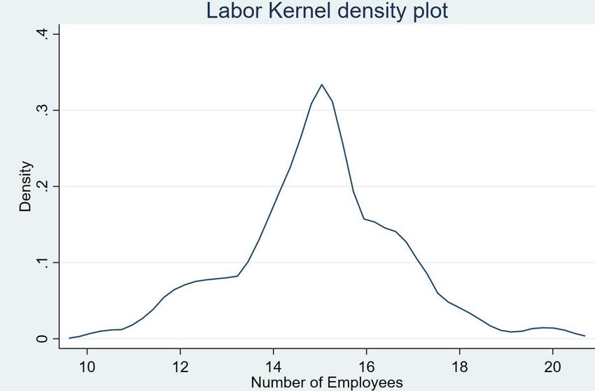
schenes and Greenstone, 2007; Mendelsohn, 2008; Ji et al., 2020). Hence, an issue
of critical importance in climate, environmental and development economics in-
volves understanding the economic impact and consequences of changes in surface
temperatures. Consequently, when estimating the impact of climate change on
gross domestic product (GDP) and total factor productivity (TFP), temperature
can not be considered as strictly exogenous (Kahn et al., 2019).
    It is a fact that year to year temperature variations constitute the most com-
mon determinant factor to specify the change of climate harmony and its effect
on the economy (Nordhaus, 2006; Dell et al., 2012; Letta and Tol, 2018). Other
than temperature variations, studies use the Wet Bulb Globe Temperature (So-
manathan et al., 2015), which is a metric that combines temperature, humidity,
precipitation and wind direction. Precipitation (annual cumulative amount of
rainfall) is the second most common analytical tool used to define climate change
(Dell et al., 2014; Damania et al., 2019). The significance of other climatic vari-
ables, such as wind speed, sunshine duration and evaporation (Zhang et al., 2017),
has recently been examined. But the vast majority of available studies investi-
gate the relationship between climate change -expressed as temperature and/or
rainfall- and economic development.
    The article at hand builds on the potential effects of temperature and pre-
cipitation, but also of CO2 emissions on countries’ economic growth estimating
a neoclassical production function. Unraveling such a relationship is in line with
a theoretical framework (Kahn et al., 2019) and empirical studies that incorpo-
rate the effects of climatic variables and CO2 emissions individually on countries’
growth. However, our intention here is to take a step further investigating the
effects of CO2 emissions and temperature in light of instrumental variables us-
ing a Cobb-Douglas production function. We argue that CO2 emissions and
temperature have an indirect impact on countries’ economic growth through an
endogenous relationship. We consider temperature, precipitation and renewable
energy sources (RES) as instruments for the CO2 emissions case, while we as-
sume precipitation and CO2 emissions as potential determinants of temperature.
This would allow us to understand not only the specific role of classical variables
of production may have on countries’ growth under this perspective, but also to
demonstrate how CO2 emissions and temperature flows are linked with countries’
growth and how they affect their climate change policies proposing an alternative
mechanism.
    The literature attempts to quantify the effects of climate change on economic
growth are relatively recent. For example, Dell et al. (2012) using country level
data find that a 1o C temperature increase in a given year reduces that year’s
economic growth by 1.3 percentage points but only in poor countries. Another
finding is that higher temperatures in poor countries tend to reduce not only the
output levels, but also the growth rates of the economy. Nordhaus (2006) detects

                                        3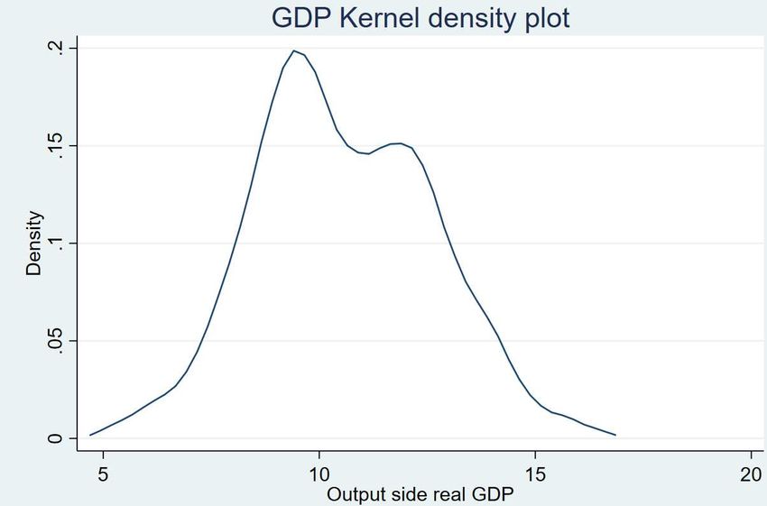
a negative relationship between temperature and output when it is measured on
a per capita basis, and a positive relationship when it is measured on a per area
basis. Leppänen et al. (2017) provide evidence in regional level that increase of
temperature reduces public expenditures for cold and hot regions, thus imply-
ing non-linear effects. Temperatures and extreme weather conditions, such as
cyclones, are expected to reduce economic output by 2.5% according to Hsiang
(2010).
    In the same line of research, Letta and Tol (2018) investigate the relation-
ship between annual temperature shocks and annual Total Factor Productivity
(TFP) growth. In agreement with Dell et al. (2012) they found a negative re-
lationship only in poor countries, where a 1o C annual increase in temperature
decreases TFP growth rates by about 1.1-1.8 percentage points. They also find
that temperature lags have an effect on countries’ economic growth implying a
persistence of weather in the medium run. They do not find existing non-linear
effects of temperature shocks on TFP. The nexus between temperature and firm
productivity is of great importance but research attempts on industry level are
scarce. Zhang et al. (2018) for half a million manufacturing plants give evidence
for the existence of an inverted U-shaped relationship between temperature and
TFP. More specifically, they estimate that an extra day with temperature ex-
ceeding 32o C reduces output by 0.45%. Somanathan et al. (2015) provide similar
evidence, concluding that productivity declines when temperature is higher than
27 degrees and that worker absenteeism increases when hot days are consecutive.
Cai et al. (2018) controlling for labor productivity show that it has an inverted U-
shaped relationship with temperature, decreasing with temperature records above
26o C. Recent evidence (Cook and Heyes, 2020) explains that cognitive workers,
despite not working outdoors, are impacted when cold temperatures are existing
outdoors.
    In order to focus the attention on factors of the production function most
studies explore the short-run relationship between pollution and labor supply,
mainly through work hours (Graff Zivin and Neidell, 2012; Hanna and Oliva,
2015). Another part of the literature explores the long-run impacts of pollution,
or contamination, mainly through diseases and illnesses (?Qiu et al., 2018) that
are in fact a spin-off of the pollution. Common finding in studies investigating the
impact of air pollution on worker productivity is that emissions have a negative
impact on productivity. When investigating for economic growth instead, the
results indicate that emissions increase economic outcomes. It is also a matter of
fact that pollution can be detrimental for infants and people suffering from other
diseases. In this line of research, Zhang et al. (2018), findings support the fact that
decreases in P M2.5 and SO2 increase labor productivity and also manufacturing
output. Hanna and Oliva (2015) present similar results for Mexico City suggesting
that decrease of SO2 emissions leads to increase of hours worked per week by

                                          4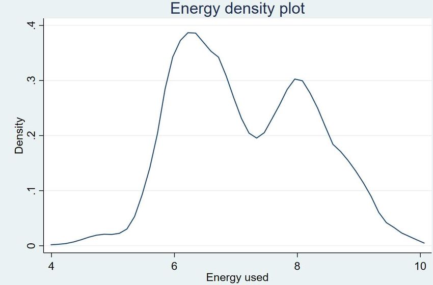
3.5%. Many could argue that the effect of emissions on labor productivity can
only be found on jobs that require human presence in open space. Chang et al.
(2019) investigate the effect of pollution on worker productivity for call centers
and find a negative relationship between the variables of interest. Similar evidence
is provided by a handful of other studies (Koundouri et al., 2010; Graff Zivin and
Neidell, 2012; He et al., 2019) suggesting that air pollution has significant negative
impacts on worker productivity.
    Finally, precipitation is whether a weak significant and positive estimator of
economic productivity (Dell et al., 2012) or not significant at all (Letta and Tol,
2018). Damania et al. (2019) focus on the impact that rainfall has on gross
domestic product. Rainfall is expressed as the total amount of precipitation that
has fallen during a year and they find that it can bring positive and statistically
significant changes in gross domestic product if the latter is calculated in sub-
national levels, unlikely with other research works that use aggregate national
levels.
    While important, the relationship between emissions and countries’ economic
growth and also the relationship between emissions and RES are not well docu-
mented in the existing literature. Kalaitzidakis et al. (2018), examine the relation-
ship between SO2 emissions and TFP growth for countries belonging to OECD.
They ascertain an increasing relationship between emissions and output and that
SO2 emissions contribute on average about 0.063% to productivity growth in the
countries of their sample. Empora and Mamuneas (2011) make use of the TFP
growth of U.S. states combined with the effect of sulphur dioxide and nitrogen
oxides and for both pollutants they conclude that TFP is positively affected. Re-
garding renewable sources Le et al. (2020) find that the use of RES helps limit
emissions but only in developed countries. The results they provide also indicate
that GHG emissions (testing for a set of different types of GHGs) have a signifi-
cantly positive effect on economic growth. It is a rational result, which is aligned
with the results we provide. Apergis and Payne (2010), testing for OECD coun-
tries, find a positive and statistically significant nexus between renewable energy
consumption and economic growth detecting bidirectional causality for the two
variables of interest.
    We contribute to the climate change economy growth literature along the fol-
lowing dimensions. Firstly, we make use of a standard Cobb-Douglas production
function and add emissions and weather variables as determinants of growth. We
consider temperature effects along with emissions which according to the available
literature has been attempted only once (Fu et al., 2018). Secondly, knowing that
emissions and temperature are responsible for climate change, it was of high im-
portance to include both of them in an equation describing the impacts of climate
change. In order to achieve this we make use of an instrumental variable regres-
sion and consider emissions and temperature as endogenous variables. Finally, we

                                          5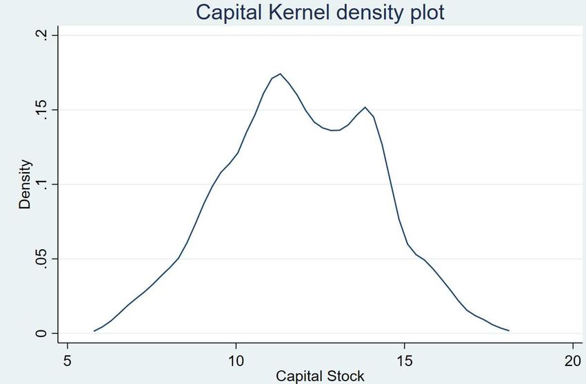
proceed with a number of alternative specification, such as robustness checks, to
examine the diversification of rich vs poor countries and possible quadratic effects.
    Drawing information from various databases and appropriately modifying it,
we construct a balanced panel dataset for the 1961-2013 period that contains
110 countries. Our main findings indicate that temperature and emissions are
negatively impacting economic development but only when we control for poor
countries, implying substantial heterogeneity between rich and poor countries.
As poor countries have to face the climate change problem more intensively, it
constitutes an extra obstacle on their way to converge with richer countries (Dell
et al., 2012; Letta and Tol, 2018; Zhang et al., 2018; Zhao et al., 2018). We
also find that TFP is declining with increasing CO2 emissions, while factors of
production have the expected signs. Non-linearity is also checked and exists for
both temperature and CO2 emissions. Existence of temperature non-linearity is
aligned with Burke et al. (2015) and Dell et al. (2012) and CO2 emissions’ non-
linearity is aligned with Kalaitzidakis et al. (2018). Finally, we find a steadily
negative relationship between emissions and share of RES. This implies that the
growing part of renewable energy can diminish the CO2 emissions concentration
and help manage the greenhouse effect (Le et al., 2020). Thus, optimal policies
should focus on clean energy generation in order to tackle emissions.
    The rest of the paper is organized as follows. Section “Methodology and empir-
ical strategy” presents the empirical background for our analysis. Section “Data
and variables” describes data sources and provides summary statistics. Section
“Empirical results and discussion presents our results while Section “Conclusions”
concludes.
2   Methodology and empirical strategy
In this section we present the methodological route we followed in order to ground
the relationship among countries’ economic growth, capital, labor, energy, carbon
dioxide emissions, temperature, precipitation and share of RES for a set of coun-
tries covering the 1961-2013 period. Based merely on Dell et al. (2012) we consider
a production function in logs estimating our primary econometric model of the
following form:

             Yit = f (Kit , Lit , Eit ) + β1 Wit + β2 CO2it + αi + πt + εit      (1)

where Wit is a vector of weather variables including annual mean temperature
and annual mean cumulative precipitation, while β2 captures the effect of coun-
tries’ emissions on their economic growth. αi depicts country fixed effects that
are caused by time invariant country characteristics and affect GDP growth.
Year fixed effects (πt ) capture annual transnational shocks to countries’ economic
growth, such as macroeconomic effects. εit is the error term and captures time

                                           6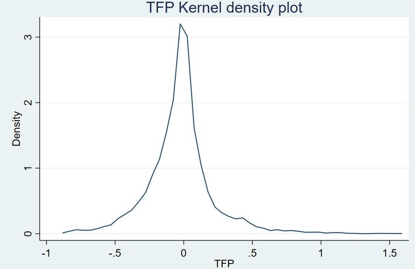
variant country characteristics that are unobservable and not included in the pa-
rameters of the estimation, but affect countries’ economic growth. In robustness
checks we allow for continents fixed effects instead of countries in order to con-
dense information that concerns countries with similarities.
    Fixed effects estimators are better than the standard regression estimators
because they are less biased and more reasonable as a method, albeit the estima-
tors may still be biased. More specifically, there still might exist unobserved time
varying differences across countries, thus implying selection bias. Using a large
dataset with a period of time of more than half a century, can lead to structural
changes within countries. These changes can derive from emissions and pollution
policies or changes in labor legislation. A second problem that gives rise to po-
tential bias is the reverse causality that results from the link between emissions
and growth (Kahn et al., 2019; Kalaitzidakis et al., 2018). It is a matter of fact
that emissions are the outcome of the production process and the more output
a country has, the more pollutants it emits. Developing economies on their way
to become developed use more emission intensive technologies and end up being
more polluted. This reverse causality problem leads to simultaneity bias when
estimated using a fixed effects method.
    We apply an instrumental variable regression strategy to remedy both of the
above mentioned biases. We consider that the link between emissions tempera-
ture and economic growth is not only straightforward as it has been described
in the majority of recent literature. According to Kaufmann et al. (2006), the
relationship between temperature and emissions does not only derive from the
fact that emissions’ concentration changes surface temperature, but also from the
fact that increases in surface temperature have caused carbon dioxide emissions’
concentration to increase. Thus, we test whether temperature, precipitation and
share of RES have an impact on carbon dioxide emissions, on the first stage re-
gressions (2) and if so, we regress economic growth on CO2 emissions, capital,
labor, energy for a given country in a given year (1):

                  CO2it = ρ0 + ρ1 Wit + ρ2 REit + αi + πt + µit                 (2)

where REit is share of RES and ρ2 the slope of the variable depicting the way
that renewable sources impact CO2 emissions. µit is the error term and the
rest of the variables have been explained at equation (1). Instruments must be
correlated with the endogenous variable, CO2 emissions in our case and have an
indirect change on the dependent variable through the endogenous. Temperature
and precipitation variables together with the share of RES are being used as
instruments for the first stage of regression. Normally, when a country increases
the quantity of energy produced from renewable sources, it is because they want
to face the increased demand for energy use or because they want to replace
the classic type of energy production with green energy from sustainable energy

                                         7
sources. In both cases, the aftermath is that the share of RES increases. This
can lead to a decrease in CO2 emissions, since it is the most common pollutant,
emitted during the production process and has to be reduced in order to prevent
temperature rise and climate change.
Finally, using the same logic we also consider that temperature operates as an
instrumental variable in Eq. (1) and examine if precipitation, denoted as P REIT
and CO2 emissions influence countries’ economic growth in the following form:
T empit = ρ0 + ρ1 C02it + ρ2 P REit + αi + πt + µit (3)
At this point we want to emphasize 5 notes. First, we choose output-side real
GDP and TFP as measures of economic growth and output. GDP, as an index
that incorporates the final market value of all goods and services, is very useful
in our era to understand the way that economic growth gets impacted by CO2
emissions and rising temperatures. On the other hand, TFP, which is the ratio
of aggregate output to aggregate inputs, can reveal the effect that emissions and
temperature have on output and productivity. TFP reveals the reactions of pro-
ductivity and combined with the fact that we use a Cobb Douglas production
function to estimate the results, it will let us have a sneak peek on more pro-
ductive characteristics of the economy. Second, we take advantage of the reverse
causality between CO2 emissions and temperature and treat them alternately as
endogenous variables and instruments. The fact that it has been proved that not
only CO2 emissions increase temperature, but also temperature increases CO2
emissions’ concentration allows to test on the endogeneity problem with two vari-
ables. Third, we try to unravel the effects of share of RES, CO2 emissions and
temperatures using continents fixed effects. We consider that the broader geo-
graphic areas can absorb some peculiarities that are common characteristics in
countries of the same continent. Fourth, following Dell et al. (2012) we create a
poor dummy in order to separate the existing country dataset in poor and rich
countries. The approach we adopt here is different and we consider a country as
poor if their GDP is below the mean GDP of all countries for that year. Thus, we
do not create only one mean GDP (that of the first year) and categorize the coun-
tries according to it, but every year’s GDP helps identify better the rich and poor
countries. Fifth, we estimate non linear effects of temperature and precipitation
in order to explore the inverted U-shaped relationship between temperature and
economic growth (Letta and Tol, 2018).
3 Data and Variables
We construct a unique panel dataset for world countries over the 1961-2013 pe-
riod. More specifically, the country-year GDP and TFP data are derived from
Penn World Table version 9.1 dataset (Feenstra et al., 2015), concerning a set of
110 countries from 1961 to 2013. We make use of variables such as output side
8real GDP (at chained PPP’s and also in million 2011 US ✩) and TFP level at
current PPP’s that are being used as the dependent variables for our estimations.
Furthermore, we make use of the capital stock (expressed at 2011 national prices)
and the number of persons engaged (in millions) for every country, in order to
create a classic Cobb-Douglas production function for estimation purposes.
Furthermore, data concerning energy is obtained from the World Bank database.
We collect data for energy use (kg of oil equivalent per capita) to represent the
energy consumed by country and by year. Energy use refers to use of primary
energy before transformation to other end-use fuels, which is equal to indigenous
production plus imports and stock changes, minus exports and fuels supplied to
ships and aircraft engaged in international transport. Data covers the years from
1960 to 2015 but we focus on 1961-2013 for 110 countries. In addition, using
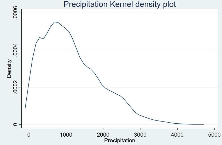
the World Bank database we collect combustible renewables and waste dataset
(expressed as a percentage of energy). The specific dataset includes energy from
solid biomass, liquid biomass, biogas, industrial waste, and municipal waste being
used in a country and measured as a percentage of total energy use. Another
innovative part of our research is making use of a second RES dataset. More
specifically, we refer to clean alternative and nuclear energy, such as hydropower,
nuclear, geothermal, and solar power. Hence, we make use of two distinct datasets
when controlling for the impact of RES on countries’ economic activity.
In addition, CO2 emissions data (metric tons per capita) is also derived from
the World Bank and includes the country-year quantities of CO2 emissions dur-
ing consumption of solid, liquid and gas fuels and gas flaring. Carbon dioxide
emissions are a by-product of fossil fuel combustion and biomass burning and
constitute the most common anthropogenic emissions affecting Earth’s radiative
balance. Carbon dioxide atmospheric concentrations have increased rapidly since
the industrial revolution and the machine introduction at the production chain.
As discussed above, we focus on the 1961-2013 period for 110 countries.
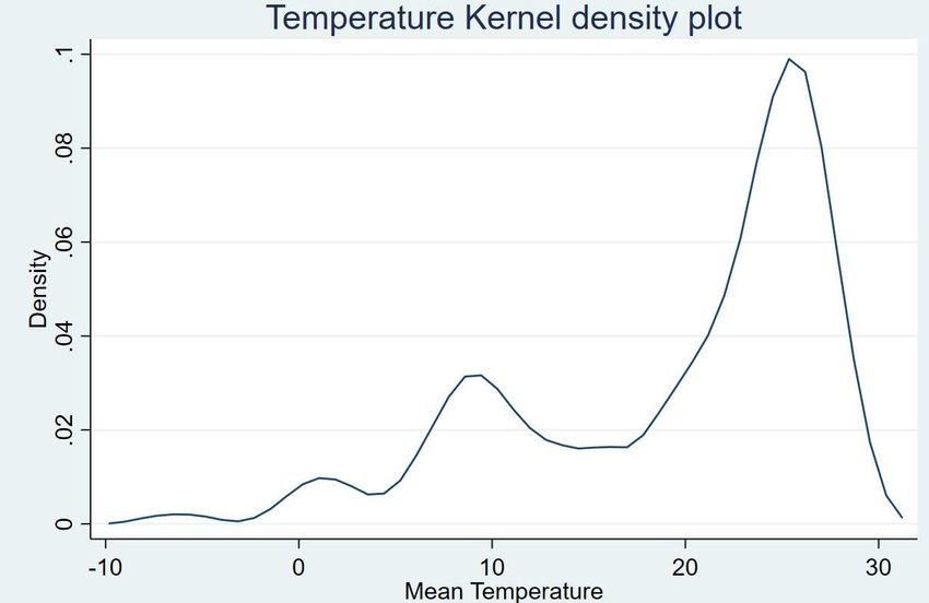
The climatic variables of temperature and precipitation have been derived from
Matsuura and Willmott (Matsuura and Willmott, 2016) and appropriately modi-
fied in gridded cells method (Nordhaus, 2006). Once collected, data are presented
on a monthly level and represent recorded temperature and precipitation from
several weather stations that have been converged into one record for a particular
geographical area according to the coordinates. Surface bounded by 0.5o latitude
and by 0.5o longitude contours (approximately 90x90 kilometers on equator) de-
picts a terrestrial unit or otherwise called, gridded cell. The specific database
covers the period 1900-2018 and with appropriate handling temperature and pre-
cipitation data can be easily extracted for the period of our interest (1961-2013).
We convert monthly temperatures and precipitation records to annual average
temperature and annual
cumulative precipitation. Then, we match them to country boundaries and con-
9struct annual average temperature and annual average cumulative precipitation
for 110 countries and 53 years. According to Nordhaus (2006), ”The grid cell is
selected because it is the unit for which data, particularly on population, are most
plentiful. From a practical point of view there is no alternative to a grid measure-
ment system”. The specific method has been used in other researches (Nordhaus,
2006; Somanathan et al., 2015) and is preferred to the method that makes use
of data that refer to one single number giving national evidence, because it can
provide more detailed information and also the geographic heterogeneity can be
dismissed.
We have to note that energy, emissions and renewable sources datasets con-
tain an unbalanced panel dataset of 290 countries for the 1950-2018 period. After
unifying the three separate datasets, we reduce the chronicle scale of our sample
to 1961-20131 . We end up having 130 countries on our dataset. Next, we merge
with the temperature and precipitation data 2 . Thus, the panel dataset consists
of 5830 observations covering 110 countries for 53 years. Table 1 presents the
logarithmic values of the variables of GDP, TFP, labor, capital, energy and CO2
emissions, which are used instead of their natural values. For all the above men-
tioned variables, plus the one representing renewable sources of energy, in order
to avoid outliers (high and low values) we replace the 0.005% highest and lowest
values with the next value counting inwards from the extremes.
4 Results and discussion
4.1 OLS and 2SLS Results
We begin by presenting the results of OLS regression together with the results
of instrumental variable regression. Table 2 is organized as follows. Panel (a)
provides the results of the first stage of the 2SLS method, while panel (b) provides
the results of the second stage and the OLS results. Each column represents a
different regression. In column (1), we provide the results of Eq.(1) which actually
is an Ordinary Least Squares method using a fixed effects strategy. As expected
(Arceo et al., 2016; Fu et al., 2018), the fixed effects estimation results are smaller
and tend to be upward toward or above zero. Columns (2), (3), (4) and (5) present
the results from the two stage regression.
In column (2) we consider CO2 emissions as the endogenous variable, meaning
that it is correlated with the error term. Endogeneity occurs because of simultane-
ity and selection bias in our case. Thus, we use CO2 as the endogenous variable
and regress it on the instruments and the exogenous variables included in our
1
We take standard procedures in the literature regarding our dataset. We drop observations
with missing values, remove outliers and reduce the number of countries by keeping those that
have at least 40 years of non-missing data on CO2 emissions.
2
For instance we find that 20 countries have no records (mainly small countries like Samoa,
Singapore and Cape Verde but also Pakistan which has very few records)
10empirical method. As instruments of the endogenous CO2 we pick a vector of
weather variables, including annual mean temperature and annual mean cumula-
tive precipitation, and the share of RES. We find that temperature has a positive
and statistically significant effect on CO2 emissions concentration, unlike precip-
itation which has a negative and statistically significant effect, but very small in
magnitude -a 1% rise in a country’s mean cumulative precipitation decreases CO2
by 0.0001%. Renewables’ estimates on the other hand, imply that they have a
strong negative effect on CO2 emissions’ concentration with a 1% increase of their
share bringing a drop in CO2 by 2.27%. On the second stage, where we estimate
the regression model including the fitted values of the instrumental variable, we
find that the three components of the production function are statistically signif-
icant. We also find that CO2 is a positive and statistically significant estimator
of GDP.
The identification tests for the specific model explain that it is well identified.
First, we reject the hypothesis that reduced form coefficients are underidentified
at 1% level. Second, we test for weak identification of all instruments using the
effective F statistic and reject the null hypothesis, concluding that all instruments
are strong (Olea et al., 2013; Pflueger and Wang, 2015).
In column (3), we change our approach in instrumental variable and consider
temperature as endogenous. According to Kaufmann et al. (2006) not only does
CO2 emissions’ concentration increase temperature, but also high temperatures
have changed the way that CO2 emissions flow in the atmosphere, thus increasing
atmospheric concentration. The fact that CO2 and temperature are being used as
instrumental variables and instruments can be explained by two facts. First, by
their relevance or in other words when each of them is used as an instrument, they
constitute a determinant factor for the endogenous. Second, as instruments they
are both conditionally uncorrelated with the error term (Cameron and Trivedi,
2005). The instruments used for the endogenous temperature are precipitation
and CO2 . Precipitation is a positive and statistically significant estimator of tem-
perature, but with a very small magnitude and CO2 is positive and statistically
significant. At the second stage of the regression, fitted values of the first stage
reveal a positive relationship between temperature and GDP. More specifically, a
1o C increase of temperature increases GDP by 0.16%. We also detect that a coun-
try’s capital stock, its labor force and total amount of energy used are positive and
significant at the 1% level. The effective F statistic of Montiel-Pflueger robust
weak identification test rejects the null of weak instruments for a weak instrument
threshold of 5% worst case bias. The underidentification test is significant at 1%
level, thus rejecting the null hypothesis that the equation is underidentified.
In column (4), the instrumental variable is CO2 but this time the depen-
dent variable is countries’ TFP instead of countries’ GDP. At the first stage of
the regression, we regress CO2 on temperature, precipitation and the share of
11RES. Temperature is a positive estimator of CO2 , while the share of RES has
a strong and negative effect on the endogenous CO2 . The precipitation holds a
small negative effect on the endogenous variable. A possible explanation of the
small magnitude that precipitation estimators have is proposed by Damania et al.
(2019). They give evidence that when precipitation data is given in large spatial
scales (country means) the impact gets negligible. It is worth mentioning that in
all specifications adopted here, the share of RES was steadily negatively related
with the CO2 emissions concentrations. At the second stage of the regression, the
intriguing result is that if CO2 increases by 1%, the TFP decreases by 0.093%.
In contrast with the CO2 -GDP relationship, when using TFP as a dependent
variable we get a negative and statistically significant estimator. TFP is a fac-
tor that encapsulates capital and labor through the use of standard production
function. Thus, TFP allows interpretation of the consequences of climate vari-
ability on more productive characteristics of the economy. Effective F statistic
is large, thus rejecting the null hypothesis that instruments are weak (Pflueger
and Wang, 2015). Last, the equation is well identified since the null hypothesis
of underidentification is rejected.
In column (5), temperature is the instrumental variable and TFP is the de-
pendent variable once again. First stage results indicate a negative effect of CO2
on temperature and a small positive effect of precipitation on temperature. The
second stage results do not provide significant evidence as the only significant
estimators are energy and temperature, which has a negative effect on TFP. In
fact, 1o C increase of temperature decreases TFP by 0.017%. In this specification
the effective F statistic of Montiel-Pflueger rises above the 5% of worst case bias
respectively.
In Table 3 we extend our research to the way that temperature and emissions
impact GDP by making two additions in our work. First, we include temperature
and CO2 first lags in order to detect the cumulative effects that temperature and
CO2 emissions have on GDP. Second, we use quadratic effects of temperature and
emissions to find whether there exists a non-linear relationship among our vari-
ables of interest and GDP. These two additions are implemented in our baseline
instrumental variable model. Thus, both the lagged variables and the quadratic
variables are being used as instruments of the endogenous CO2 emissions and
temperature, as they were introduced in previous analysis.
Column (1) of Table 3, first lag of temperature is positioned as an instrument
of endogenous CO2 emissions, together with temperature, precipitation and the
share of RES. During first stage regression, neither temperature nor its lag yield
significant results, in contrast with RES variable and precipitation, albeit the
precipitation estimator is very small. Second stage results provide a positive and
significant estimator of endogenous CO2 emissions and the rest of the estimators
results are similar to results in Column (2) of Table 2. Thus, we do not find
12strong evidence for temperature persistence on CO2 emissions. In column (2), we
change our approach to the endogenous and treat temperature as such. The first
stage regression results are close to being considered as significant at 10% level.
Second stage results are similar to the results presented in Column (3) of Table
2.
Columns (3) and (4) examine the impact of quadratic values of temperature
and emissions, respectively. Quadratic value of temperature enters the first stage
regression with CO2 emissions being regarded as endogenous. We observe that
temperature has a positive and statistically significant impact on CO2 emissions,
while quadratic value of temperature is negative and significant at 5% level. At
the second stage of the regression, CO2 emissions are estimated to have a positive
and statistically significant coefficient. The result is aligned with Kalaitzidakis et
al. (2018). Second stage results are very similar to the baseline results presented
in Table 2. When quadratic value of emissions is considered as an instrumental
variable of temperature, the results imply non-linearity with CO2 emissions having
a positive value and quadratic CO2 emissions being negative and significant. At
the second stage, temperature has a strong and significant impact on GDP (in
accordance with Dell et al. (2012)). In each case, we conclude that temperature
and CO2 emissions have a non-linear effect on growth through the channel of
endogeneity that we have established.
In table 4, we insert a dummy variable depicting whether a country is consid-
ered poor or not. We do that in order to reveal the existing heterogeneity among
countries and how that affects the relationship that we examine. The threshold
used to distinguish rich and poor countries is the first quartile of GDP values
of all countries over the whole period. A country is defined as poor if its GDP
for a given year is less than sample’s GDP first quartile. That way, a country
can change rich/poor status within years and does not remain rich or poor ac-
cording to first year comparisons (as in Dell et al. (2012)). It is crucial because
we work with a dataset that covers a 53-year period of time and therefore we
assume that changes in rich/poor status of countries are certain. Column (1)
endogenous variable is the interaction between CO2 emissions and poor dummy.
We find a stronger link between temperature interacted with a poor dummy and
the endogenous, than temperature and CO2 as presented in Table 1. The most
interesting result is that when a poor dummy is interacted with CO2 then its im-
pact on a country’s economy becomes negative and statistically significant, thus
indicating substantial heterogeneity between rich and poor countries. Specifically,
a 1% increase of CO2 emissions decreases economic growth by 0.021%. Column
(2) uses temperature interacted with poor dummy as endogenous variable and
at the first stage we get a strong influence of CO2 interacted with the endoge-
nous. At the second stage of the regression, once again substantial heterogeneity
between rich and poor countries is revealed. This time we find a negative and
13statistically significant temperature interacted with poor dummy and countries’
GDP. In fact, a 1o C rise in temperature decreases GDP by 0.011%. The results
presented in Table 4 and having in mind results of Table (2), we conclude that
effects of temperature and emissions are only detected in poor countries. For both
specifications examined in Table 4, the effective F statistic critical values is large,
thus rejecting the null hypothesis that instruments are weak. This conclusion is
similar to previous important findings (Dell et al., 2012; Letta and Tol, 2018).
Poor countries are facing the dangers of increasing temperatures more intensively
than rich countries, but the dangers do not stop there since we provide evidence
that increasing CO2 emissions also deteriorate the position of an economy.
4.2 Robustness checks
Table 5 shows the robustness checks under different assumptions. We start by pro-
viding the results from using alternative RES instead of combustible renewables
and waste dataset. The specific robustness check results strengthen our baseline
results that RES have a strong negative impact on CO2 emission concentrations
by reducing them by 1.79% when the share of RES increases by 1%. Further-
more, on the second stage analysis, we detect a negative relationship between the
endogenous variable which is CO2 and GDP that plays the role of the depen-
dent variable. Increasing CO2 by 1% brings a drop in GDP by 0.15%, indicating
that increasing CO2 emissions can be harmful for a country’s economy. At the
same time capital, labor and energy variables, all of them components of a Cobb-
Douglas production function, are positive and statistically significant. Regarding
the instrumental variable regression and whether the variables used are adequate,
we examine the effective F statistic of Montiel-Pflueger and find that the result
of the test is large, thus rejecting the null hypothesis that instruments are weak.
In column (2), we consider CO2 as the endogenous variable and countries’
TFP as the dependent variable. Results here are similar to the results presented
at column (4) of Table 2. Once again, we find a negative and statistically signif-
icant relationship between alternative RES and CO2 emissions. Also, we reveal
that CO2 at the second stage, have a negative effect on countries’ TFP index.
Specifically, a 1% increase of emissions, reduces countries’ TFP by 0.12%. The
effective F statistic of Montiel-Pflueger test, once again rejects the null hypothesis.
In columns (3) and (4) of Table 3, we change the variable depicting carbon
emissions and instead of using CO2 emissions concentration we examine the CO2
intensity for all countries during the period 1961-2013. We construct carbon
emission intensity by dividing the carbon
dioxide emission quantities to each country’s GDP per year. It is an index that
can be used to measure the carbon emission performance on country level. Thus,
we exploit this property and use it as an alternative way of capturing the impact
of CO2 emissions on economic growth. The results remain quite similar with
those presented in columns (1) and (2). More specifically, we detect the negative
14relationship that exists among alternative RES share and CO2 emissions intensity.
Furthermore, at the second stage regression the endogenous CO2 intensity has a
negative effect on the dependent variable, whether we use GDP or TFP as it. The
identification tests are performing well indicating that the IV regression equation
is well identified.
5 Conclusions
Many scholars argue that understanding the relationship between precipitation,
temperature and CO2 emissions on economic growth and productivity is critical
to the design of optimal mitigation policies. Economists, on their part, have tried
to measure the damage of climate change and quantify the relationship between
the above-mentioned variables. However, a major conceptual dilemma arises from
the relationship among economic growth, temperature and CO2 emissions, since
many authors argue that increased GHGs in the atmosphere alter average temper-
ature and consequently could reduce economic growth. On the other hand, faster
economic activity increases GHGs and consequently global average temperature
(Nordhaus, 1992).
This paper explores the importance of CO2 emissions, RES, temperature and
precipitation in estimating the economic growth of climate change in a sample of
world countries. We employ a standard Cobb-Douglas production function and
add weather variables and CO2 emissions as factors. We investigate if weather
conditions affect gross domestic product and total factor productivity using a
production function. Also, we argue that anthropogenic emissions are responsi-
ble for the increase of temperature that has been conducted since the industrial
revolution (Kaufmann et al., 2006) and that the use of RES should alter the cli-
mate change phenomenon. Thus, we employ an instrumental variable approach
where CO2 emissions and temperature affect GDP and TFP through the use of
instruments such as weather variables, share of RES and also emissions.
In our study we exploit of a data set composed of 110 countries for the 1961-
2013 period. Our findings confirm the positive effect of emissions and temperature
on countries’ economic growth while disentangling the specific effect when we
account for poor vs rich countries. In that specification it is revealed that poor
countries are more vulnerable to CO2 emissions and temperature increases and
this distinction is considered to be an important factor of inequality. Therefore,
we can assume that temperature and emissions are two so far underestimated,
yet important factors of countries’ inequality. Actually, if a country is considered
poor then a 1% increase of CO2 emissions decreases economic growth by 0.021%
and a 1o C rise in temperature decreases GDP by 0.011%. The magnitude of
the RES estimator in all baseline regressions was exceeding 1.7% while having a
negative effect. That is a strong estimator implying that a 1% increase of RES
share can have a drop in CO2 emissions concentration by at least 1.78%. The
15importance of RES for the combat against climate change is underlined by our
results. In fact, for all specifications the share of RES was used as an instrument
for endogenous CO2 provided a negative estimator and an interpretation for this is
that RES decrease CO2 emissions concentration and increase of their share in total
amount of energy used could mean less CO2 and better environmental conditions.
Finally, our results also provide evidence for the existence of an inverted U-shaped
relationship for temperature and emissions while the factors of production appear
to have the expected signs.
A possible future research we would like to conduct is the effect of carbon
emissions and weather variables on gross domestic product on a regional level.
The regional level cross-examination will detect deeper and more precisely the
impact of emissions and rising temperatures on growth. The smaller geographical
areas will reveal much more detailed relationships for the variables of interest and
will lead us to more secure estimators. A second research question that arouses
our curiosity is what will happen if instead of a Cobb-Douglas, we use an alter-
native production function.
Acknowledgments
The authors would like to express their sincere gratitude to Professors Kostas
Tsekouras, Nicholas Giannakopoulos, Oreste Napolitano, Nikos Chatzistamoulou
and postdoctoral researcher Eirini Stergiou for valuable comments and help.
16Appendix
Figure 1: Kernel density plots of regression variables
17Table 1: Sample Statistics
Standard
Variables Mean deviation Observations Minimum Maximum
GDP (in million 2011 US✩) 10.581 2.06 5641 5.01 16.54
TFP level at current PPP’s -0.022 0.24 3927 -0.85 1.56
Capital stock 11.921 2.25 5641 6.13 17.73
Labor force 14.991 1.68 5174 10.17 20.46
Energy 7.170 1.04 3993 4.16 9.88
CO2 emisions 9.076 2.58 5781 1.29 15.76
CO2 intensity 0.342 0.34 5617 0.5 3.56
Combustible
Share of Renewables 0.229 0.27 3967 0 0.97
Clean Alternative
Share of Renewables 0.067 0.10 3965 0 0.71
Country Temperature 19.392 7.38 5830 1.05 29.07
Country Precipitation 161.68 6.80 4611 0.10 4162.6
*All variables except for Country Temperature and Country Precipitation are presented
here in their logarithmic values. Combustible and Clean Alternative Share of
Renewables are shares.
18Table 2: OLS and 2SLS estimates
(1) (2) (3) (4) (5)
OLS 2 SLS
Panel (a) First stage
Endogenous Variable: CO2 Temp CO2 Temp
Temperature 0.016∗∗∗ 0.007∗∗∗
(0.0016) (0.0014)
Precipitation −0.0001∗∗∗ 0.00∗∗∗ −0.000∗∗∗ 0.001∗∗∗
(0.0000) (0.0001) (0.0000) (0.0001)
Renewable −2.369∗∗∗ −1.782∗∗∗
(0.0506) (0.0475)
CO2 0.323∗∗∗ −0.378∗∗∗
(0.1150) (0.1468)
Panel (b) Second stage
Dependent Variable: GDP GDP GDP TFP TFP
Capital 0.334∗∗∗ 0.488∗∗∗ 0.509∗∗∗ 0.032∗∗∗ −0.008
(0.0177) (0.0170) (0.0142) (0.0113) (0.0078)
Labor 0.126∗∗∗ 0.346∗∗∗ 0.455∗∗∗ 0.055∗∗∗ 0.002
(0.0207) (0.0150) (0.0123) (0.0118) (0.0077)
Energy 0.031∗ 0.202∗∗∗ 0.186∗∗∗ 0.089∗∗∗ .030∗∗∗
(0.0177) (0.0200) (0.0222) (0.0177) (0.0094)
CO2 emissions 0.160∗∗∗ 0.148∗∗∗ −0.093∗∗∗
(0.0144) (0.0206) (0.0167)
Temperature 0.016∗∗ 0.162∗∗∗ −0.017∗∗
(0.0076) (0.0142) (0.0037)
Year fixed effects Y Y Y Y Y
Countries fixed effects Y N N N N
Regions fixed effects N Y Y Y Y
F Eff 962.8 51.4 572.0 91.2
Sample Size 4063 4028 4063 3349 3354
*All models include year fixed effects. Model of column (1) also includes country fixed
effects, while the rest include region fixed effects. Column (2) and (4) first stage
endogenous variable is CO2 and column (3) endogenous variable is temperature. Sample
period: 1961-2013 for 110 countries. Standard errors are clustered in parentheses.
Statistical significance is noted as follows: ∗ ∗ ∗p < 0.01, ∗ ∗ p < 0.05, ∗p < 0.1
19Table 3: 2SLS estimates using lags and non-linearity
(1) (2) (3) (4)
Panel (a) First stage
Endogenous Variable: CO2 Temp CO2 Temp
Temperature 0.002 0.021∗∗∗
(0.0091) (0.0028)
Precipitation −0.000∗∗∗ 0.001∗∗∗ −0.1∗∗∗ 0.000
(0.0000) (0.0001) (0.0113) (0.0000)
Renewable −2.376∗∗∗ −2.313∗∗∗
(0.0509) (0.0512)
CO2 0.451 0.669∗∗∗
(0.4879) (0.2544)
Temperature lag 0.013
(0.0091)
CO2 lag -0.149
(0.4856)
T emperature2 −0.002∗∗∗
(0.0001)
Emissions2 −0.038∗∗∗
(0.0132)
Panel (b) Second stage
Dependent Variable: GDP GDP GDP GDP
Capital 0.487∗∗∗ 0.510∗∗∗ 0.484∗∗∗ 0.285∗∗∗
(0.0206) (0.0118) (0.0205) (0.0396)
Labor 0.345∗∗∗ 0.454∗∗∗ 0.356∗∗∗ 0.584∗∗∗
(0.0150) (0.0122) (0.0149) (0.1102)
Energy 0.202∗∗∗ 0.189∗∗∗ 0.212∗∗∗ 0.088∗∗∗
(0.0200) (0.022) (0.0197) (0.0349)
CO2 emissions 0.150∗∗∗ 0.145∗∗∗
(0.0206) (0.0205)
Temperature 0.161∗∗∗ −0.397∗∗∗
(0.0142) (0.1266)
Year fixed effects Y Y Y Y
Countries fixed effects N Y N Y
Regions fixed effects Y N Y N
Sample Size 4005 4039 4028 3822
F ef f 761.2 33.2 717.0 3.8
*All models include year fixed effects. Sample period: 1961-2013 for 110 countries.
Standard errors are clustered in parentheses. Statistical significance is noted as follows:
∗ ∗ ∗p < 0.01, ∗ ∗ p < 0.05, ∗p < 0.1
20Table 4: 2SLS estimates interacting a dummy for country being poor with tem-
perature and CO2 emissions respectively
(1) (2)
Panel (a) First stage
Endogenous Variable: CO2 ×poor Temp×poor
Temp×poor 0.299∗∗∗
(0.0043)
Precipitation −0.0003∗∗∗ 0.0006∗∗∗
(0.0001) (0.0000)
Renewable −0.872∗∗∗
(0.0940)
CO2 ×poor 2.272∗∗∗
(0.0698)
Panel (b) Second stage
Dependent Variable: GDP TFP
Capital 0.559∗∗∗ 0.539∗∗∗
(0.0125) (0.0132)
Labor 0.422∗∗∗ 0.423∗∗∗
(0.0126) (0.0131)
Energy 0.336∗∗∗ 0.301∗∗∗
(0.0137) (0.0143)
CO2 × poor −0.021∗∗∗
(0.0043)
Temp× poor −0.011∗∗∗
(0.0018)
Year fixed effects Y Y
Regions fixed effects Y Y
F Eff 2025 849.7
Sample Size 4028 4063
*All models include year fixed effects and regions fixed effects. Column (1) first stage
endogenous variable is CO2 interacted with a dummy variable for poor countries, while
in Column (2) the first stage endogenous variable is temperature interacted with the
dummy variable for poor countries. Sample period: 1961-2013 for 110 countries.
Standard errors are clustered in parentheses. Statistical significance is noted as follows:
∗ ∗ ∗p < 0.01, ∗ ∗ p < 0.05, ∗p < 0.1
21Table 5: 2SLS estimates using alternative renewable energy sources and CO2
emissions intensity
(1) (2) (3) (4)
Panel (a) First stage
Dependent Variable: CO2 CO2 intensity
Temperature −0.008∗∗∗ −0.021∗∗∗ −0.011∗∗∗ −0.009∗∗∗
(0.0022) (0.0016) (0.0013) (0.0012)
Precipitation −0.001 0.000∗∗∗ −0.000∗∗∗ −0.000∗∗∗
(0.0001) (0.0000) (0.0000) (0.0000)
Alternative
Renewable −1.796∗∗∗ −1.935∗∗∗ −1.08∗∗∗ −1.057∗∗∗
(0.0645) (0.0604) (0.0440) (0.0459)
Panel (b) Second stage
Dependent Variable: GDP TFP GDP TFP
Capital 0.635∗∗∗ 0.045∗∗∗ 0.513∗∗∗ −0.028∗∗∗
(0.0225) (0.0104) (0.0115) (0.0076)
Labor 0.509∗∗∗ 0.076∗∗∗ 0.476∗∗∗ 0.016∗∗
(0.0211) (0.0120) (0.0119) (0.0079)
Energy 0.420∗∗∗ 0.118∗∗∗ 0.415∗∗∗ 0.065∗∗∗
(0.0262) (0.0154) (0.0146) (0.0120)
CO2 emissions −0.152∗∗∗ −0.126∗∗∗
(0.0310) (0.0153)
CO2 intensity −0.468∗∗∗ −0.171∗∗∗
(0.0436) (0.0267)
Year fixed effects Y Y Y Y
Regions fixed effects Y Y Y Y
F Eff 179.7 336.1 164.4 209.9
Sample Size 4024 3345 4025 3346
*All models include year fixed effects and regions fixed effects. Column (1) and (2) first
stage endogenous variable is CO2 , while in Column (3) and (4) first stage endogenous
variable is CO2 intensity. Sample period: 1961-2013 for 110 countries. Standard errors
are clustered in parentheses. Statistical significance is noted as follows:
∗ ∗ ∗p < 0.01, ∗ ∗ p < 0.05, ∗p < 0.1
22References
Apergis, N., & Payne, J. E. (2010). Renewable energy consumption and
economic growth: evidence from a panel of OECD countries. Energy policy,
38(1), 656-660.
Arceo, E., Hanna, R., & Oliva, P. (2016). Does the effect of pollution on infant
mortality differ between developing and developed countries? Evidence from
Mexico City. The Economic Journal, 126(591), 257-280.
Batten, S. (2018). Climate change and the macro-economy: a critical review.
Benavides, M., Ovalle, K., Torres, C., & Vinces, T. (2017). Economic growth,
renewable energy and methane emissions: is there an enviromental Kuznets
curve in Austria?. International Journal of Energy Economics and Policy,
7(1).
Brown, P. T., Li, W., Jiang, J. H., & Su, H. (2016). Unforced surface air
temperature variability and its contrasting relationship with the anomalous
TOA energy flux at local and global spatial scales. Journal of Climate, 29(3),
925-940.
Burke, M., Hsiang, S. M., & Miguel, E. (2015). Global non-linear effect of
temperature on economic production. Nature, 527(7577), 235-239.
Caron, J., & Fally, T. (2018). Per capita income, consumption patterns, and
CO2 emissions (No. w24923). National Bureau of Economic Research.
Cai, X., Lu, Y., & Wang, J. (2018). The impact of temperature on man-
ufacturing worker productivity: evidence from personnel data. Journal of
Comparative Economics, 46(4), 889-905.
Cameron, A. C., & Trivedi, P. K. (2005). Microeconometrics: methods and
applications. Cambridge university press.
Chang, T. Y., Graff Zivin, J., Gross, T., & Neidell, M. (2019). The effect of
pollution on worker productivity: evidence from call center workers in China.
American Economic Journal: Applied Economics, 11(1), 151-72.
Chen, S., Oliva, P., & Zhang, P. (2018). Air pollution and mental health:
evidence from China (No. w24686). National Bureau of Economic Research.
Cline, W. R. (1992). The economics of global warming. Institute for Interna-
tional Economics, Washington, DC, 399.
Cline, W. R. (2007). Global warming and agriculture: Impact estimates by
country. Peterson Institute.
Cook, N., & Heyes, A. (2020). Brain freeze: outdoor cold and indoor cognitive
performance. Journal of Environmental Economics and Management, 102318.
Damania, R., Desbureaux, S., & Zaveri, E. (2019). Does rainfall matter for
economic growth? Evidence from global sub-national data (1990–2014). The
World Bank.
Dell, M., Jones, B. F., & Olken, B. A. (2014). What do we learn from the
weather? The new climate-economy literature. Journal of Economic Litera-
23You can also read