Examining the Economic Impact of COVID-19 in India through Daily Electricity Consumption and Nighttime Light Intensity - World Bank Document
←
→
Page content transcription
If your browser does not render page correctly, please read the page content below
Public Disclosure Authorized

                               Policy Research Working Paper                             9291
Public Disclosure Authorized

                                     Examining the Economic Impact
                               of COVID-19 in India through Daily Electricity
                                 Consumption and Nighttime Light Intensity
                                                                 Robert C. M. Beyer
Public Disclosure Authorized

                                                               Sebastian Franco-Bedoya
                                                                    Virgilio Galdo
Public Disclosure Authorized

                               South Asia Region
                               Office of the Chief Economist
                               June 2020
Policy Research Working Paper 9291
Abstract
The COVID-19 pandemic has disrupted economic activity somewhat subsequently, but electricity consumption was
in India. Adjusting policies to contain trans- mission while on average still 13.5 percent lower than normal in May. Not
mitigating the economic impact requires an assessment all states and union territories have been affected equally.
of the economic situation in near real-time and at high While electricity consumption halved in some, others were
spatial granularity. This paper shows that daily electricity not affected at all. Part of the heterogeneity is explained by
consumption and monthly nighttime light intensity can the prevalence of manufacturing and return migration. At
proxy for economic activity in India. Energy consumption the district level, higher COVID-19 infection rates were
is compared with the predictions of a consumption model associated with larger declines in nighttime light intensity
that explains 90 percent of the variation in normal times. in April. Together, daily electricity consumption and night-
Energy consumption declined strongly after a national lock- time light intensity allow monitoring economic activity in
down was implemented on March 25, 2020 and remained a near real-time and high spatial granularity.
quarter below normal levels throughout April. It recovered
This paper is a product of the Office of the Chief Economist, South Asia Region. It is part of a larger effort by the World
Bank to provide open access to its research and make a contribution to development policy discussions around the world.
Policy Research Working Papers are also posted on the Web at http://www.worldbank.org/prwp. The authors may be
contacted at rcmbeyer@worldbank.org, sfranco2@@worldbank.org, and vgaldo@worldbank.org.
The Policy Research Working Paper Series disseminates the findings of work in progress to encourage the exchange of ideas about development
issues. An objective of the series is to get the findings out quickly, even if the presentations are less than fully polished. The papers carry the
names of the authors and should be cited accordingly. The findings, interpretations, and conclusions expressed in this paper are entirely those
of the authors. They do not necessarily represent the views of the International Bank for Reconstruction and Development/World Bank and
its affiliated organizations, or those of the Executive Directors of the World Bank or the governments they represent.
Produced by the Research Support TeamExamining the Economic Impact of COVID-19
in India through Daily Electricity
Consumption and Nighttime Light Intensity
Robert C. M. Beyer1 Sebastian Franco-Bedoya2 Virgilio Galdo3
Keywords: COVID-19, lockdown, electricity consumption, nighttime light intensity, India
JEL codes: E01, E65, O53, Q43, R11
1
World Bank, email: rcmbeyer@worldbank.org.
2
World Bank, email: sfranco2@worldbank.org.
3
World Bank, email: vgaldo@worldbank.org.
This paper should not be reported as representing the views of the World Bank. We are grateful to Hans
Timmer, Valerie Mercer-Blackman, Phil Hammons, Dhruv Sharma, Rangeet Gosh, and Rishabh Choudhary for
excellent comments and suggestions.1 Introduction
The Coronavirus Disease 2019 (COVID-19) pandemic has disrupted economic activity in India.
Until mid-March 2020, the economy was mainly hit by disruptions in cross-border connections.
For example, tourism arrivals in India declined due to strict travel restrictions and some value
chains were interrupted, especially with China. When COVID-19 started to spread in India
through domestic contagion, the Indian authorities enacted a series of measures to combat the
pandemic, including a national lockdown from March 25 onwards that strongly disrupted eco-
nomic activity across the country. When restrictions were stepwise eased in May, economic
activity slowly recovered. Shutdowns and other non-pharmaceutical interventions to contain the
spread of COVID-19 have high economic costs and consequently tend to be accompanied by
policy responses to mitigate their economic impact (Gourinchas 2020). In line, both the Reserve
Bank of India and the Government of India announced measures to assist individuals and com-
panies that were negatively affected. Adjusting containment measures and policy responses to
mitigate their economic impact require an assessment of the magnitude of the economic situation
in near real-time. In addition, since the impact can vary at different locations, an assessment at
high spatial granularity is needed.
Indicators traditionally used to monitor the economic situation are available only with
substantial lags and often at the national level only, and hence provide little insights into the
immediate effect of strong and sudden policy measures like a national lockdown. In response
to such problems, economists have suggested different proxies that are available at a higher
frequency and with shorter publication lags, as well as at a higher spatial granularity. Two of
these are electricity consumption and night light intensity. Electricity is an input to activities
throughout the economy, from industrial production to commerce and household activity, so
changes in consumption reveal information about these activities in real-time (Cicala 2020a,
2020b). Similarly, nighttime light intensity contains information about economic activity at
high spatial granularity. Such proxies have become especially important during the COVID-19
pandemic, as it makes data collection through surveys, which are fundamental for the traditional
estimation of gross value added, more difficult. In line, the Central Statistical Office noted that
data collection challenges related to India’s national lockdown will likely result in revisions to its
growth estimate for the first quarter of 2020.
Both electricity consumption and nighttime light intensity closely track economic activity
1and have been used extensively to improve national account estimates of GDP (e.g. Henderson
et al. 2012, Lyu et al. 2018, Chen et al. 2019). Both proxies have also been used to assess
the economic impact of major policy measures. Nighttime light intensity, for example, allowed
assessing the impact of India’s demonetization in November 2016 (Beyer, Chhabra, Galdo, and
Rama 2018, Chodorow-Reich, Gopinath, Mishra, and Narayanan 2020). It is also invaluable
to approximate economic activity at the sub-national level, including in India (Gibson, Datt,
Murgai, Ravallion 2017, Prakash, Shukla, Bhowmick, and Beyer 2019, Chanda and Kabiraj
2020). In concurrent work, electricity consumption has been shown to have closely tracked
economic activity in the United States during the global financial crisis (Cicala 2020a).4 And it
has been employed for an assessment of the economic impact of the COVID-19 pandemic in the
European Union (Cicala 2020b, Chen et al. 2020b).5
In this paper, we first confirm a meaningful relationship between electricity consumption,
nighttime light intensity, and economic activity in India. We then propose a new real-time mea-
sure of daily economic activity in India at the country and state levels based on daily electricity
consumption. We estimate an electricity consumption model based on the day of the week, the
week of the year, the temperature, and holidays that explains 90 percent of the variation in In-
dia’s electricity consumption. Comparing the actual electricity consumption in 2020 to the one
predicted by the model allows us, first, to quantify the economic costs of the COVID-19 pan-
demic and the national lockdown implemented on March 25, 2020 and, second, to understand
different impacts between states. In addition, we use night light intensity to gauge the impacts
at the district and city level and to explore their local drivers.
We find a strong impact of the national lockdown on India’s electricity consumption. It
dropped on average 28.5 percent in the week after its implementation and was on average still
25.8 percent below normal throughout April. It started recovering in early May and was nearly
back to normal between May 23 and May 28, before dropping again at the end of the month to
-14.7 percent on May 31.6 Not all Indian States and Union territories have been affected equally.
While electricity consumption halved in some, it did not decline at all in others. It declined more
for States and Union territories with a larger manufacturing sector and higher previous short-
4
While real GDP fell 4.3 percent from peak to trough, weather-adjusted electricity consumption fell around 5
percent (Cicala 2020a).
5
Energy consumption at the beginning of April 2020 was down by around 10 percent with large differences
between countries due to varying impacts of the pandemic and containment measures (Cicala 2020b).
6
The deviation is statistically significant at the one percent level from March 23 to May 24 and from May 29
to May 31.
2run outmigration, but not with more registered COVID-19 cases. However, districts with higher
rates of COVID-19 infections saw larger declines in nighttime light activity in April, suggesting
additional impacts from voluntary behavioral changes when risks of an infection increase (in line
with evidence provided by Melony and Taskin 2020). In nearly all large Indian cities nighttime
light intensity was lower in April 2020 than it was a year earlier. In Delhi and Chennai, for
example, light intensity declined by around 10 percent.
The rest of the paper is structured as follows. In Section 2, we describe the measures
implemented by the Indian authorities and discuss their impact on mobility. The data is pre-
sented in Section 3 and the relationship of electricity consumption, nighttime light intensity, and
economic activity in Section 4. In Section 5, we present the electricity consumption model and
examine the impact of the national lockdown at the country level. In Section 6, we compare the
impact across states and in Section 7 we examine the change in nighttime light intensity at the
district and city level. Section 8 discusses the wider economic implications of our results and
concludes.
2 Measures by Indian authorities to contain the pandemic
On March 22, 2020, India observed a 14-hour long curfew to combat the COVID-19 pandemic
and assess the country’s ability to implement containment measures. The government already
ordered a lockdown in 75 districts where COVID-19 cases had occurred, as well as in all major
cities. Further, on March 24, the government ordered a nationwide lockdown for 21 days, effective
from March 25 until April 14, affecting the entire 1.3 billion population of India.7
After the enactment of the national lockdown, nearly all public offices were closed, and
public services suspended.8 In addition, nearly all commercial and private establishments had
to be closed and exceptions were only made for essential businesses like banks and insurance
offices, internet and printing services, and shops selling food (which were encouraged to provide
home delivery). Industrial establishments were closed, and exceptions were only made for man-
ufacturing units producing essential commodities. Such units required permission from the state
governments to operate. Moreover, all but essential transport services – whether by air, rail, or
roadways – were suspended and so were hospitality services. Finally, all educational institutions
were closed as well. The lockdown, intended to end on April 14, was initially extended until
7
MHA order no. 40-3/2020-DM-I(A).
8
Exceptions were given to several essential services like police forces and public utilities.
3May 3. However, in areas where no new cases of COVID-19 arose until then, the government
partially released restrictions from April 20 onwards. Agricultural activities were allowed again
along with public works under the Mahatma Gandhi National Rural Employment Guarantee Act
(MNREGA). In addition, industries operating in rural areas, Special Economic Zones (SEZs),
industrial estates and industrial townships could operate again, if they had arrangements for
workers to stay on the premises. And construction activity in rural areas could continue as well.
On May 1, the Ministry of Home Affairs extended the lockdown for a period of two weeks
from May 4 until May 17. However, many restrictions were relaxed or lifted. For example,
the central government permitted again the inter-state movement of migrant workers, pilgrims,
tourists and others that were stranded during the nationwide lockdown and the Ministry of
Railways began to operate special trains with social distancing measures to facilitate movements.
Based on risk profiling, India’s authorities divided districts into green, orange, and red zones.
The profiling depends, among other things, on the amount of COVID-19 cases, recovery rates,
and the extent of testing and surveillance. As of April 30, there were 130 red zone districts, 284
orange zone districts and 319 green zone districts. In green zones, restrictions were eased strongly,
and most economic activity could resume. In addition, all goods traffic was permitted again, and
individuals could move freely again for non-essential activities from 7 AM to 7 PM. However,
air, rail, metro and inter-state road travel remained prohibited and educational institutions,
hospitality services and places of large public gatherings (such as cinemas and malls) remained
closed. In orange zones, restrictions were also relaxed, but some related to mobility remained. In
red zones, industrial establishments in urban areas remained prohibited from operating, except
for those in Special Economic Zones and industrial estates/townships with access control. And
while private offices could operate again even in red zones, a maximum of a third of the employees
could be physically present in the office at the same time. Finally, construction remained mostly
prohibited in red zones. On May 17, the lockdown was again extended but new relaxations
were announced. For the first time, states were given authority to determine the specifics of the
lockdown. In addition, two new zones (containment and buffer) were added to the red, orange,
and green zones.
The national lockdown enacted by the Indian authorities was successful in limiting mobil-
ity. Figure 1.a uses the Google Mobility Reports for India (Google 2020) to show how mobility
declined after the lockdown was enacted. This data is based on tracking smartphones, which
in India have a coverage of 27.7 percent (Newzoo 2018). While this means that not everyone
4(a) Mobility in India after the lockdown (b) Weekly unemployment in India
Note: (a) The decline refers to the change of visits and length of stay as of May 16, compared to a baseline period. The
baseline period is defined as the median value for the corresponding day of the week, during the 5-week period from
January 3 to February 6. The mobility trends for retail and recreation places include restaurants, cafes, shopping centers,
theme parks, museums, libraries, and movie theaters. (b) The unemployment rates are produced by CMIE based on
household interviews using its Consumer Pyramids Household Survey machinery.
Source: (a) Google COVID-19 Community. (b) Centre for Monitoring Indian Economy Pvt. Ltd.
Figure 1: Mobility and unemployment in India after the lockdown
is tracked, the mobility data is still based on a very large sample and can hence be used to
assess declines in mobility across the world (Maloney and Taskin 2020). The noticeable drop in
workplace presence around March 10 was due to Holi. Shortly before the national lockdown was
announced on March 24, the presence at workplaces had already declined by over 10 percent and
by a similar magnitude in retail and recreation locations. When the lockdown was implemented,
the presence at the workplace dropped immediately by half and a few days later by an additional
20 percent. At the same time, residential places were frequented more often, confirming that In-
dians indeed stayed at home more due to the lockdown. Since mid-April, presence at workplaces
slowly increased again but on May 16, presence at workplaces was still 40 percent below normal.
The economic impact of the lockdown was immediate. The weekly unemployment rate
reported by the Centre for Monitoring Indian Economy (CMIE 2020) increased from 10 percent
both in urban and rural areas in the week before the lockdown to 30 percent in the week thereafter
in urban areas, and to 20 percent in rural areas (Figure 1.b). Different from developments in other
countries, unemployment rates did not increase further after that and since then are hovering
around 25 percent both in urban and rural areas. The increase in unemployment is evidence
of a severe and sustained negative economic impact, which also manifests itself in other data.
5For example, cargo traffic and rail freight declined, oil demand collapsed, and India’s Purchase
Manager Index dropped to an all-time low in April. An excellent discussion of the economic
impact of COVID-19 on India’s economy is provided by Dev and Sengupta (2020).
3 Data
3.1 Daily Electricity Consumption
We observe daily electricity consumption from April 1, 2013 to May 31, 2020. The data is
measured and collected from the Power System Operation Corporation Limited (POSOCO),
which is a government-owned enterprise under the Ministry of Power. It is responsible for
ensuring the integrated and reliable operation of India’s grid. POSOCO makes available daily
reports of electricity consumption with one-day delay. We download the daily documents and
scrap the electricity information to build our electricity consumption database for India. While
the total electricity consumption in these documents does not differentiate between different uses
(residential, commercial, etc.), it does breakdown the electricity consumption of the different
states. This will later allow us to track the specific impact of the lockdown on the different
states.
Figure 2 shows India’s daily electricity consumption from April 1, 2013 to May 31, 2020.9
A couple of features are clearly noticeable. First, until the end of 2019, there is a clear upward
trend with electricity consumption on average growing 4.3 percent each year. Second, there
is a clear seasonality in the data with electricity consumption being higher between May and
September than at the beginning and end of the year. Third, there was a noticeable decline
already at the end of 2019, long before the COVID-19 pandemic disrupted economic activity in
India.10 Fourth, around the national lockdown announced on March 24, electricity consumption
dropped strongly. Fifth, at the end of May electricity consumption first recovered before falling
again.
3.2 Nighttime light intensity
The nighttime light data are extracted from the VIIRS-DNB Cloud Free Monthly Composites
(version 1) made available by the Earth Observation Group at the National Geophysical Data
9
The figure is in mega units. A mega unit is one million units of electricity, where one unit is equal to one
kilowatt hour.
10
This decline at the end of 2019 has been linked to weakening GDP growth.
6Figure 2: India’s electricity evolution since April 2013
Note: In India, the kilowatt-hour is called a Unit of energy. A million units, designated MU, is a gigawatt-hour. The last
day included is May 31, 2020.
Center of the National Oceanic and Atmospheric Administration (NOAA) and cover the period
from April 2012 to April 2020. The data from the VIIRS satellites have a resolution of 15-arc
seconds (0.5 km x 0.5 km tiles near the equator) and, compared to a previous nighttime light
product known as DMSP-OLS (Elvidge et al. 2013), have a wider radiometric detection range
and onboard calibration. These features help to correct for saturation as well as blooming effects
and ensure a better time comparability. However, the raw data needs some cleaning to minimize
temporary lights and background noise. In this paper, we reduce the background noise with
two procedures similar to Beyer et al. (2018). The first approach takes advantage of the 2015
annual composite of stable VIIRS nighttime light to identify a background noise mask (Elvidge
et al. 2017). Only cells lying outside this background noise mask are treated as stable lights,
while those inside the mask are recoded with value zero, corresponding to no light. The second
approach follows Elvidge et al. (2017) and translates their cleaning algorithm based on defining
a background noise mask with a clustering method using daily data, to monthly data. While we
lose some accuracy with this approach in 2015, it takes into account all later observations for
7creating the best possible mask for our period of analysis. And for 2015, the two approaches result
in very similar light data. Clusters are identified by removing outlier observations, averaging
cells over time, and clustering areas based on their nighttime light intensity. In practice, this
approach amounts to setting to zero cells that are distant from homogenous bright cores. We
present results based on data cleaned with the second method, but our results are robust to both
cleaning methods. For this paper, cleaned monthly data are aggregated to the district and city
levels and standardized by area. Nighttime light is measured in Nanowatts/cm2 /steradian.
3.3 Other variables
Data on quarterly economic activity measured as gross value added (GVA) is from the Central
Statistics Office. Temperature data is collected from the Average Daily Temperature Archive
from the University of Dayton (2020) and based on recordings of the National Climatic Data
Center. We generate an India aggregate by weighting the daily temperatures recorded in Chennai,
Delhi, Kolkata, and Mumbai by population.11 Data on Indian holidays is from different online
sources. The information about registered COVID-19 infections at the state and district level
is from Covindia (2020), the data on previous short-run inmigration and outmigration at the
state and district level from the Development Data Lab (2020), and the share of employment in
manufacturing and services at the state and district level is from the South Asia Spatial Database
(Li, Rama, Galdo, and Pinto 2015).
4 Electricity, nighttime lights, and economic activity
Intuitively, electricity consumption and economic activity are closely related since most economic
activity needs electricity. Plenty of studies analyze the relationship of the two over longer periods,
often with a focus on the direction of causality. Chen, Kuo, and Chen (2007), for example,
study 10 newly industrializing and developing Asian countries and find a bi-directional long-run
causality between real GDP and electricity consumption and a uni-directional short-run causality
running from economic growth to electricity consumption. Ferguson, Wilkinson, and Hill (2000)
find that correlations between electricity consumption and GDP are close to one. In Appendix
A, we use a sample of 123 countries to update these correlations between economic growth
11
The weighting is done at the regional level (according to the POSOCO classification) where Chennai represents
the South, Delhi the North, Kolkata the East and North-East, and Mumbai the West.
8and electricity consumption. We find that electricity consumption increased by 0.95 percent
for each percent additional economic activity. For India, electricity increased slightly above 1
percent. Similarly, data on nighttime lights has also shown to be able to track economic activity.
Henderson et al. (2012) develop a statistical framework to use satellite data on night lights
to augment official income growth measures. They show that for countries with poor national
income accounts, the optimal estimate of growth is a composite with roughly equal weights on
conventionally measured growth and growth predicted from lights.
In this section, we explore the usefulness of electricity consumption and satellite night
light as proxies for economic activity in India. To do so, we estimate the following quarterly (t)
model:
log GV At = β1 log electricityt + β2 log lightt + trendt + qt + εt (1)
where the log of GVA is regressed on the log of electricity consumption and the log of
nighttime light intensity. In addition, we include a trend and quarter fixed effects, qt , to control
of the intra-year seasonality of the data. We aggregate the electricity consumption and nighttime
light data to quarterly frequency to match the frequency of the GVA and estimate the model for
the period from the second quarter of 2013 to the first quarter of 2020.12
Table 1: GVA, electricity and nighttime lights
(1) (2) (3) (4) (5) (6) (7) (8) (9)
log GVA log GVA log GVA log GVA log GVA log GVA log GVA log electricity log electricity
log electricity 1.296∗∗∗ 0.350∗∗∗ 0.318∗∗∗
(0.061) (0.078) (0.104)
log night light 1.537∗∗∗ 0.179∗∗ 0.035 1.205∗∗∗ 0.451∗∗∗
(0.175) (0.066) (0.073) (0.112) (0.115)
log electricity (demean) 0.191∗∗∗
(0.067)
log night light (demean) 0.149∗∗∗
(0.031)
trend 0.012∗∗∗ 0.015∗∗∗ 0.012∗∗∗ 0.008∗∗∗
(0.001) (0.001) (0.001) (0.001)
constant -6.047∗∗∗ 5.664∗∗∗ 8.999∗∗∗ 9.874∗∗∗ 6.038∗∗∗ 0.000 0.000 11.597∗∗∗ 12.083∗∗∗
(0.763) (0.969) (0.142) (0.046) (1.253) (0.001) (0.001) (0.090) (0.080)
Quarter FEs YES YES YES YES YES NO NO YES YES
N 28 28 28 28 28 28 28 28 28
r2 0.953 0.994 0.775 0.992 0.994 0.238 0.477 0.846 0.958
Standard errors in parentheses
∗ ∗∗ ∗∗∗
p < .1, p < .05, p < .01
12
The beginning of the sample coincides with the availability of the electricity daily data.
9Table 1 shows the results of regressing GVA on electricity consumption and nighttime light
intensity. Columns 1 and 2 show that electricity consumption and GVA move together closely
both in levels and as deviations around a trend. In both cases the relationship is statistically
significant at the one percent level. For each percentage point increase in electricity consumption,
GVA grew 1.3 percentage points. This relationship is very similar to the one-to-one relationship
Cicala (2020a) finds for the United States, including during the global financial crisis, and even
closer to the elasticity of 1.4 that Chen et al. (2020) find in Europe.13 Columns 3 and 4
replicate the regressions for nighttime light, showing that it also follows the evolution of GVA
very closely.14 However, GVA shares more of its variation with electricity consumption than with
nighttime light intensity, as reflected in a lower R2 of the latter regression. This could be due to
larger measurement errors in nighttime lights compared to electricity consumption. Since both
move together with economic activity, they are related. Consequently, nighttime light turns out
not to be significant when we include both electricity and light in the same regression (column
5). In columns 6 and 7, we demean the data by regressing GVA, electricity consumption and
nighttime lights on year and quarter fixed effects. We then regress the residuals of GVA on
the residuals of electricity and lights. This allows us to understand the relationships between
the quarterly fluctuations of GVP, electricity and lights. Columns 6 and 7 confirm that both
electricity and lights are able to track quarterly fluctuations, with both coefficients turning out
to be significant at the one percent level. Finally, we regress electricity on lights to examine how
strongly they are correlated in India. Columns 8 and 9 show a strong relationship both in levels
and around a common trend. A 1 percent increase in light intensity is associated with a 1.2
percent increase in electricity consumption.
Electricity consumption seems to have a somewhat stronger relationship, especially when
both variables are combined. We therefore rely on electricity consumption to track economic
activity at the country and state level, for which electricity data is available, and rely on nighttime
light intensity for districts and cities.
13
It is also in line with other estimates in the literature (Stern 2018).
14
With 1.5, our coefficient is much larger than the one Henderson et al. (2012) find in an annual panel regression
using the DMSP-OLS data (their Table 2, column 1). One reason could be that VIIRS data allows for greater
comparability over time as explained in section 3.2.
105 The impact of COVID-19 on electricity consumption in India
5.1 Modeling daily electricity consumption
To understand the magnitude of the decline of electricity consumption due to the lockdown, we
need to control for factors affecting electricity consumption like the season and the weather. We
hence estimate the following model of electricity consumption using daily (t) data:
log Electricityt = τt + DWt + W Yt + Holidayt + β1 Coolingt + β2 Heatingt + βt T rend + εt (2)
The explanatory variables are a set of fixed effects that control for the day of the week,
DWt , the week of the year, W Yt , and holidays, Ht . We include two variables that control for
the daily temperature. We control for the temperature degrees above and below of 22.8◦ C, such
that Coolingt = max{tempt − 22.8◦ C, 0} and Heatingt = max{22.8◦ C − tempt , 0}, respectively.
This temperature is associated with the minimum electricity consumption in India, which we
confirmed by regressing log electricity consumption on temperature and a quadratic term of
temperature suggesting that electricity consumption increases above and below this temperature
(see Appendix B). The variables of interest are the set of dummy variables τt that indicate each
day in 2020 until the last day of the sample. These variables capture how daily consumption in
2020 differs from consumption in previous years, conditional on the temperature and holidays.15
As discussed above, electricity consumption in India grew over time and hence we include a linear
time trend (trend). This model is estimated separately for India and for all Indian states and
Union territories.
Table 2 presents the estimation results for different versions of the electricity consumption
model. Until December 2019, the upward trend in electricity consumption alone explains over
70 percent of the variation (column 1). Since electricity consumption dropped below the trend
in 2020, an estimation until the end of May 2020 results in a less steep trend that explains
somewhat less of the variation (column 2). When we add the daily fixed effects for 2020 as
described above, only the observations until December 2019 determine the coefficient on the
trend (column 3).16 Figure 2 shows that there is some seasonality in electricity consumption,
which we control for by including the week of the year. Taking care of the trend, the deviation
15
As an alternative, one can also estimate the model until the end of December 2019 and compute the (out-of-
sample) prediction errors. These are identical to the daily fixed effects.
16
Note that the explanatory power is now slightly above the one for the model only estimated until December
2019 because the daily fixed effects take out the errors in 2020.
11Table 2: Electricity consumption dynamics model
(1) (2) (3) (4) (5) (6) (7)
log electricity log electricity log electricity log electricity log electricity log electricity log electricity
Trend 0.133∗∗∗ 0.115∗∗∗ 0.133∗∗∗ 0.137∗∗∗ 0.137∗∗∗ 0.133∗∗∗ 0.133∗∗∗
(0.002) (0.002) (0.002) (0.001) (0.001) (0.001) (0.001)
Holiday -0.022∗∗∗ -0.022∗∗∗
(0.003) (0.003)
Cooling 0.021∗∗∗ 0.021∗∗∗
(0.001) (0.001)
Heating -0.001 -0.001
(0.001) (0.001)
End of data Dec 2019 May 2020 May 2020 May 2020 May 2020 Dec 2019 May 2020
2020 daily FEs NO NO YES YES YES NO YES
Week of the year FEs NO NO NO YES YES YES YES
Day of the week FEs NO NO NO NO YES YES YES
N 2143 2292 2292 2292 2292 2143 2292
R2 0.711 0.608 0.729 0.860 0.872 0.896 0.902
∗ ∗∗ ∗∗∗
Standard errors in parentheses. p < .1, p < .05, p < .01
from trend in 2020, and the seasonality already explains over 80 percent of the variation in
electricity consumption (column 4).17 Next, we also include the days of the week to account for
within-week variation, which results for example from different activities over weekends (column
5). Finally, we add holidays and the two variables for cooling and heating periods, as described
above. On holidays, the electricity consumption tends to be 2.2 percent lower than on usual
days and the effect is statistically significant at the one percent level. Of the two temperature
variables, only the one for heating is significant at the one percent level. If temperature exceeds
22.8◦ C, electricity consumption increases on average by 2.1 percent for every one ◦ C increase in
temperature (column 5). With 90 percent, the variation explained by our preferred specification
is very high and hence it is well suited to analyze deviations from its predictions.18
5.2 Changes in Indian electricity consumption and nighttime light intensity
Figure 3 plots the estimated daily deviation of actual electricity consumption from the model
prediction from the beginning of 2020 until May 31, and the dashed lines show the 95 percent
confidence interval.19 From the beginning of the year, with the exception of Holi, the deviations
17
As an alternative to the week of the year, we also included the month. Since it resulted in a slightly lower fit
of the model, we use the week of the year in the baseline estimation.
18
The increase of the explanatory power by the inclusion of daily 2020 fixed effects for 2020 is only half a
percent (column 6).
19
These are the daily dummies for 2020 that we include in the estimation. They absorb the variation unexplained
by the model and are identical to (out-of-sample) prediction errors. Using instead the latter and identifying outliers
based on robust standardized residuals, as suggested by (Kirachi 2013), results in the same days with below normal
electricity consumption (see Appendix C).
12Figure 3: Deviations from predicted electricity consumption in India from January 1, 2020 and
until May 31, 2020.
hover around the model’s prediction and are not statistically significantly different from them
until Sunday, March 22.20 That day, however, the national curfew caused a drop in electricity
consumption to 15 percent below predicted levels, and that drop is statistically significant at the
one percent level. On Monday, March 23, a day before the national lockdown was announced,
electricity consumption was 16 percent lower than predicted and it declined further to -21 percent
on Tuesday, the day the national lockdown was announced. After the lockdown was enacted, elec-
tricity consumption dropped further and on March 27 and 28, electricity consumption troughed
at more than 30 percent below normal levels. Subsequently, it started to recover slightly, and
deviations were around -25 percent throughout April. Following the different relaxations of the
lockdown, electricity consumption increased again in May. Between May 23 and May 28, while
still somewhat below normal levels, electricity consumption was not statistically significantly
different from the model prediction at one percent anymore, suggesting that economic activity
has had largely resumed. However, it dropped again subsequently and on May 31 electricity
consumption was again -14.7 percent below prediction. On average, electricity consumption in
20
While not statistically significant, actual electricity consumption fell below the prediction already from mid-
February onwards, which may indicate first economic disruptions due to broken cross-border connections.
13Note: States are ordered according to average deviations over all three months. Only negative deviations from
model prediction are shown.
Figure 4: Changes in electricity consumption across Indian states
May was 13.5 percent below normal levels, and hence roughly half way back compared to April.
With the exception of the rebound and subsequent decline at the end of May, the changes in elec-
tricity consumption follow closely the Oxford stringency index of government interventions used
for international comparisons of containment measures.21 Going forward, it will be interesting to
see whether electricity consumption will remain below normal levels, returns to previous levels,
or whether it will even overshoot to compensate for foregone activity during the lockdown.
6 Heterogeneity across Indian states
The decline in electricity consumption after the lockdown was not uniform across Indian states.
Figure 4 shows the deviation from the model prediction for March, April, and May by running
the model in Equation (2) at the state level.22 The average deviations from normal levels over
all three months vary from below -30 percent in Himachal Pradesh and Uttarakhand to small
positive deviations in Karnataka and Sikkim. In most of the states, electricity consumption
21
We plot the change in electricity consumption against the stringency index in the Appendix D.
22
For this we fit a separate model for each state. The temperature used to determine heating and cooling
periods is the same for every state.
14declined most strongly in April. The decline in April was strongest in Himachal Pradesh, where
electricity consumption nearly halved. The negative deviation from the model prediction was also
larger than 20 percent during this month in Uttarakhand, Goa, Arunachal Pradesh, Meghalaya,
Delhi, Gujarat, Punjab, Assam, Chhattisgarh, Odisha, and Telangana. On the other side of the
spectrum, there are some states for which electricity consumption in April was nearly unaffected.
In Jharkhand, Karnataka, Manipur, and Nagaland, the deviation from the model prediction
was only between 5 percent and 3 percent, and in Sikkim it was even slightly above (but not
statistically significant). In May, the electricity consumption was still more than 20 percent below
normal in Himachal Pradesh and Uttarakhand, but it was already back to normal levels in nine of
the states, including in Punjab, Haryana, and Rajasthan. The heterogeneity is even larger across
Union territories.23 In March, the decline was largest in DNH and DD, where the deviation from
the model’s prediction was over 35 percent. In Puducherry and Jammu and Kashmir, on the other
hand, the deviation in March was only around 3 percent. The national lockdown affected most
Union Territories very strongly in April, when actual electricity consumption was 86 percent,
71 percent, and 56 percent below normal in DNH, DD and DVC, respectively. The monthly
deviations of actual from predicted electricity consumption and the explanatory power of the
electricity consumption model for all States and Union Territories are reported in Appendix F.
In order to understand some of the heterogeneity in electricity changes across states, we
first analyze the effect of the number of registered COVID-19 cases (per capita) and the share of
manufacturing employment, which approximates the share of manufacturing production. Both
are expected to be positively correlated with the decline in electricity consumption. The former
for two reasons: first, a higher number of cases makes it more likely that people voluntarily
reduce mobility (Maloney and Taskin 2020) and, second, because a higher number of registered
cases makes it more likely that state governments enact the lockdown more strictly. The latter
because manufacturing output tends to be more electricity intense than output in services and
agriculture. Table 3 reports the estimation results for a cross-section of States and Union terri-
tories in April and May. For the full sample, both variables have the expected sign but are not
statistically significant even at the 10 percent level. Restricting the sample to those states and
Union territories for which our model explains at least half of the variation reduces the num-
ber of observations from 29 to 28, and results in a statistically significant effect of the share of
manufacturing. As expected, a higher share of manufacturing is associated with a larger decline
23
See figure in the Appendix E.
15Deviation of electricity in April/May
(1) (2) (3)
COVID-19 cases -0.273 -0.290 0.614
(0.237) (0.218) (0.319)
Share of manufacturing -0.187 -0.387** -0.609***
(0.177) (0.184) (0.186)
Share of services -0.215
(0.181)
Past in-migration -0.245***
(0.0794)
Past out-migration 0.623***
(0.178)
Constant -0.0810** -0.0565 0.0414
(0.0392) (0.0377) (0.136)
Number of observations 29 28 28
R2 of elect. consumption model all >0.5 >0.5
R2 0.076 0.181 0.525
Standard errors in parentheses. * p∆ Electricity consumption in April 2020
(1) (2) (3)
∆ light intensity, April 2020 0.579** 0.892*** 1.251***
(0.230) (0.287) (0.519)
∆ light intensity squared, April 2020 -2.789*
(1.607)
Constant -0.188*** -0.138*** -0.135***
(0.0277) (0.0393) (0.04)
N 30 30 26
light intensity all allNote: Arunachal Pradesh, Dadra Nagar Haveli, and Daman and Diu are dropped from the analysis. The green
line is a linear approximation conditional on ∆ < 0.1; the black solid line a linear approximation for the full
sample, and the dashed black line a quadratic approximation.
Figure 5: Relationship between changes in electricity consumption and changes in nighttime
light intensity at the state level
quarterly one emerging from the time-series dimension at the country level (Table 2, column 8).
We conclude that in the absence of electricity data, nighttime light intensity offers a valuable
alternative to analyze economic activity.
7 Using night light intensity to look below the state level
7.1 District-level changes in nighttime light intensity
In absence of high-frequency official statistics at low levels of spatial disaggregation, data collected
from outer space has become a reliable alternative. The use of satellite-derived data has made
substantive inroads in the recent economic literature (Burchfield et al. 2006, Donaldson and
Storeygard 2016). Nighttime light data has been extensively used in a wide array of economic
studies ranging from monitoring economic activity (Henderson et al. 2012, Keola et al. 2015,
Henderson et al. 2018) to assessing regional economic convergence (Chanda and Kabiraj 2020)
to identifying urban spaces and markets (Gibson et al. 2017, Baragwanath et al. 2019, Galdo et
al. 2019, Ch et al. 2020) to predicting welfare (Jean et al. 2016), and to assessing the quality
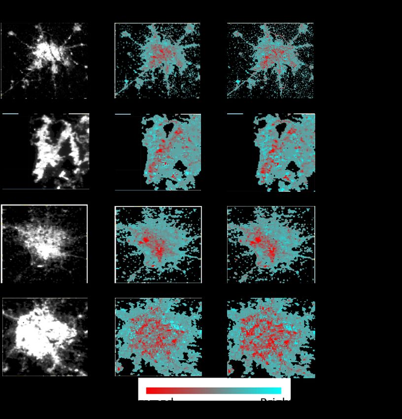
18(a) ∆ April 2020 (b) (∆ April 2020) – (avg. ∆ April 2017-19)
Figure 6: Changes in night light intensity across Indian districts in April 2020
of national account statistics (Pinkovskiy et al. 2016, Morris and Zhang 2019), among other.
More recently, nighttime light data has been used to evaluate the economic impact of India’s
demonetization in November 2016 (Beyer et al. 2018, Chodorow-Reich et al. 2020).
The changes in nighttime light intensity due to the COVID-19 pandemic and the national
lockdown were heterogeneous across districts in India, but some spatial patterns are clearly
recognizable. Figure 6 (a) shows the year-on-year change in light intensity in April 2020.25 The
map clearly shows that the decline in light intensity was larger among districts in the north-west
and south-east than in others. More than two-thirds of the districts experienced an absolute
decline in light intensity in April 2020 compared to a year before – and one-fifth of the districts
experienced declines above 15 percent. The average (median) decline in nighttime intensity
across districts was 12 percent (10 percent). Over the last years, nighttime light intensity has
been increasing strongly in some districts, while it is only moderately increasing in others. Instead
of the absolute change, we hence analyze the change in the growth rate of districts’ light intensity.
In order to reduce noise in the data, we compare the growth in light intensity in April 2020 to the
average growth in April the three years before. Figure 6 (b) shows that about 80 percent of the
districts experienced a decline of their light intensity growth in April of 2020. For half of them,
the decline was larger than 15 percentage points. The average (median) decline in nighttime
light intensity growth across districts was 18 percentage points (15 percentage points).
Next, we examine drivers of the observed heterogeneity across districts in the change of
25
The year-on-year change accounts for seasonality in the data.
19nighttime lights intensity in April 2020. To do so, we link the change to the number of COVID-
19 cases per million residents, the share of manufacturing employment, as well as to migration
patterns (as we did before for states).26 Column 1 in Table 5 replicates the first column of Table
3 for districts and shows that there is, as expected, a positive and significant correlation between
the share of manufacturing employment and the decline in nighttime light intensity. A larger
share of manufacturing is associated with larger decreases in light intensity as the lockdown cut
important light emissions sources. A one percentage point increase in the share of manufacturing
employment is associated with a decline in light intensity of 0.19 percentage points. The numbers
of COVID-19 cases per million residents, though negative in sign, is not statically significant at
the ten percent level. Measurement issues of COVID-19 infections at district level could be a
source of noise in the data hiding a linear relationship. We hence create four categorical variables
of COVID-19 infections: the first category takes the value of 1 if a district does not register any
case and zero otherwise; the second category takes the value of 1 if a district registered cases
but less than 10 per million residents and zero otherwise; the third category takes the value of
1 if a district registered between 10 to 50 cases per million residents and zero otherwise; and
the fourth category takes the value of 1 if a district registered more than 50 cases per million
residents and zero otherwise. In addition, we also control for past in and out-migration. Columns
2 and 3 in Table 5 report the results of this analysis. They show a significant positive correlation
of COVID-19 cases and the decline in light intensity. Districts with more COVID-19 cases per
million residents experienced larger declines in light intensity. While having had less than 10
COVID-19 cases per million residents was associated with a 3.7 percent points larger decline in
light intensity, having had more than 50 COVID-19 cases per million residents was associated
with a 12.6 percentage points larger decline. Note that in April districts were not yet divided
into different categories and hence these results suggest that with higher local risks of infection,
people either followed the national lockdown more strictly or changed their behavior voluntarily.
While the share of service employment has a negative and significant correlation with declines in
light intensity, the share of manufacturing employment is positively correlated with the decline
though statistically insignificant. In line with the results at the state level, previous out-migration
is negatively correlated with declines in light intensity, suggesting that those districts with a lot
of past out-migration have experienced substantive return migration after the lockdown was
enacted.
26
Districts from Arunachal Pradesh are excluded from the analysis.
20∆ nighttime light intensity ∆ nighttime light intensity 1/ ∆ nighttime light intensity 1/
(1) (2) (3)
COVID-19 cases -0.00369
(0.00272)
Less than 10 COVID-19 cases -3.294** -3.687***
(1.412) (1.415)
Between 10 to 50 COVID-19 cases -6.896*** -7.340***
(1.720) (1.733)
More than 50 COVID-19 cases -10.97*** -12.65***
(2.749) (2.970)
Manufacturing employment share -0.198*** -0.0780 -0.0905
(0.0667) (0.0700) (0.0712)
Service employment share 0.114**
(0.0518)
Past in - migration -0.146
(0.161)
Past out - migration 0.583*
(0.339)
N 624 624 623
R2 0.017 0.052 0.063
Note: 1/ Base category: no COVID-19 cases as of Apr 30, 2020. Standard errors in parentheses. *** pAt a more granular level, it is possible to observe the change in light intensity in April
2020 within cities. Since the data on nighttime light intensity is available at a very fine grid, their
aggregation is very flexible. In the following, we aggregate data for India’s 26 largest metropolitan
areas. For selected mega cities, Figure 7 shows the light intensity in April 2020 (first column)
and whether light intensity dimmed or brightened in April 2020 (column 2). Subtracting the
light intensity in April 2019 from the one in April 2020 controls for seasonality in light emissions.
The maps in column 2 clearly indicate a substantive decline in light intensity in April 2020, as
shown by the many reddish cells that show an absolute decline. As in the analysis of states, we
compare the growth rate in April 2020 to the average growth rate in April over the last three
years and show results in column (3). This “dif-in-dif" analysis confirms that declines April 2020
were not part of a general trend but specific to that month.
Figure 8: Changes in nightlight intensity across major Indian cities in April 2020
Figure 8 shows the change in light intensity in April 2020 compared to a year before for
the 25 largest Urban Metropolitan Areas in India. As for states and districts, the economic
impact of the lockdown varied across them. While nearly all of them report declines in light
intensity in April 2020, the declines range from 16.8 percent in Nagpur to 0.5 percent in Pune.
And for Kolkata and Patna, located in Bihar and West Bengal in the north-east of India, light
22intensity did not decline at all. The average (median) decline in nighttime light intensity across
these major metropolitan areas was 8.1 percent (8.3 percent). Nagpur, the city with the largest
decline in light intensity in April 2020, is the third largest city of the state of Maharashtra,
India’s fifth fastest growing city, and a top performer in the smart city project execution. In the
metropolitan area of Delhi, nighttime light intensity declined by 13 percent. Using a sample of 54
cities and proxying city-level COVID-19 cases with district-level information, we find a significant
positive correlation between COVID-19 cases per million residents and decline in light intensity.
Having more than 50 cases per million residents is associated with a 15 percentage points larger
decline in light intensity.
8 Conclusion
In this paper, we showed that both electricity consumption and nighttime light intensity can
proxy economic activity in India. We then quantified the drop in electricity consumption in
response to the COVID-19 pandemic and the national lockdown, which the Indian authorities
implemented from March 25 onwards. Compared to predicted consumption based on a model
explaining 90 percent of the variation in electricity consumption, actual electricity consumption
declined around 20 percent shortly after the lockdown was implemented. It fell further subse-
quently, to a maximum decline of 30 percent at the end of March. It was around 25 percent
below normal throughout April and subsequently recovered somewhat, following the stepwise
relaxation of restrictions, but was on average still 13.5 percent lower than normal in May.
The observed decline in electricity consumption clearly says something about the overall
economic costs that have occurred during this period. To estimate the costs emerging from our
measure, we consider all days for which electricity consumption has been statistically significantly
lower than predicted.27 We utilize the elasticity of 1.3 between changes in electricity consumption
and GVA that we estimated in Section 4 and that is very much in line with typical values found
in the literature. Doing so suggests that year-on-year quarterly growth in the first quarter of
2020 was 3.4 percentage points lower than it would have otherwise been. For the second quarter
of 2020, it suggests that the negative growth effect until the end of May has already been 17.0
percentage points. For the full calendar year, this amounts to economic costs of 5.1 percent
of GVA so far, or to around US$ 150 billion. This estimate is a bit lower but roughly in line
27
We use a significance level of 1 percent.
23with approximations reported in the media. The actual growth in the second quarter of 2020
will of course depend on whether the economy will continue to be held back by the COVID-19
pandemic, whether it will revert to previous levels, or whether it will overshoot to compensate
for forgone activity during the lockdown. The strength of the rebound can also be well tracked
by our measure based on daily electricity consumption.28
We also document that the economic impact of the lockdown was not equal across states,
districts, and cities. Some of the heterogeneity in the decline in electricity consumption is related
to the economic structure of the states and previous migration patterns. We find that a larger
number of COVID-19 infections resulted in a larger decline in nighttime light intensity in districts,
but not in states.
Concluding, electricity consumption tracks GVA fluctuations closely and has been used
to assess the economic impact of lockdowns in the European Union. We showed that electricity
consumption can also be used in emerging markets and developing economies. For India, we
can update this measure of economic activity with only a one-day delay, which provides a near
real-time view on economic activity. This provides a valuable source of information for policy
makers and researchers alike. We also provided a first assessment of the impact at the district
and city level based on nighttime light intensity that can be further refined as more data becomes
available.
28
In a recent note Chinoy and Sajjid (2020: 2) agree that the energy consumption will be an “important real-time
tracker to judge the extent to which economic utilization levels increase in the coming weeks”.
24References
Baragwanath, K., Goldblatt, R., Hanson, G. and Khandelwal, A.K. (2019). Detecting urban
markets with satellite imagery: An application to India. Journal of Urban Economics, In press.
Beyer, R. C., Chhabra, E., Galdo, V., Rama, M. (2018). Measuring districts’ monthly economic
activity from outer space (No. 8523). World Bank Policy Research Working Paper.
Burchfield, M., Overman, H.G., Puga, D. and Turner, M.A. (2006). Causes of sprawl: A portrait
from space. The Quarterly Journal of Economics, 121(2), 587-633.
Chanda, A. and Kabiraj, S. (2020). Shedding light on regional growth and convergence in India.
World Development, 133, 104961.
Ch, R., Martin, D.A. and Vargas, J.F. (2020). Measuring the size and growth of cities using
nighttime light. Journal of Urban Economics, p.103254.
Chen, S. T., Kuo, H. I., Chen, C. C. (2007). The relationship between GDP and electricity
consumption in 10 Asian countries. Energy Policy, 35(4), 2611-2621.
Chen, S., Igan, D., Pierri, N., Presbitero, A. F. (2020). Tracking the Economic Impact of
COVID-19 and Mitigation Policies in Europe and the United States. International Monetary
Fund Special Series on COVID-19.
Chen, W., Chen, X., Hsieh, C. T., Song, Z. (2019). A Forensic Examination of China’s National
Accounts. Brookings Papers on Economic Activity, 77-127.
Chinoy S. Jain, T. (2020). India begins calibrated exit from lockdown; macro impact beginning
to get visible. JP Morgan Chase, Asia Pacific Emerging Markets Research.
Chodorow-Reich, G., Gopinath, G., Mishra, P., Narayanan, A. (2020). Cash and the economy:
Evidence from India’s demonetization. The Quarterly Journal of Economics, 135(1), 57-103.
Cicala, S. (2020a). Electricity Consumption as a Real Time Indicator of Economic Activity.
Unpublished Manuscript.
Cicala, S. (2020b). Early Economic Impacts of COVID-19 in Europe: A View from the Grid.
Unpublished Manuscript.
Covindia (2020). Covindia, https://github.com/covindia.
Development Data Lab (2020). Covid-19 Data Resources, https://github.com/devdatalab/covid
Dev, S. M., Sengupta, R. (2020). Covid-19: Impact on the Indian economy. Indira Gandhi
Institute of Development Research, Mumbai, April.
Donaldson, D. and Storeygard, A. (2016). The view from above: Applications of satellite data
25in economics. Journal of Economic Perspectives, 30(4),171-98.
Elvidge, C. D., Baugh, K. E., Zhizhin, M., Hsu, F. C. (2013). Why VIIRS data are superior
to DMSP for mapping nighttime lights. Proceedings of the Asia-Pacific Advanced Network, 35,
62-69.
Elvidge, C. D., Baugh K. E., Zhizhin, M., Chi, F., Ghosh, T. (2017). VIIRS night-time lights.
International Journal of Remote Sensing, 38(21): 5860-5879.
Ferguson, R., Wilkinson, W., Hill, R. (2000). Electricity use and economic development. Energy
Policy, 28(13), 923-934.
Galdo, V., Li, Y. and Rama, M., (2020). Identifying urban areas by combining human judgment
and machine learning: An application to India. Journal of Urban Economics, In press.
Gibson, J., Datt, G., Murgai, R., Ravallion, M. (2017). For India’s rural poor, growing towns
matter more than growing cities. World Development, 98, 413-429.
Gourinchas, P. O. (2020). Flattening the pandemic and recession curves, in Richard Baldwin
and Beatrice Weder di Mauro (eds), Mitigating the COVID Economic Crisis: Act Fast and Do
Whatever It Takes, CEPR Press.
Henderson, J.V., Squires, T., Storeygard, A. and Weil, D. (2018). The global distribution of
economic activity: Nature, history, and the role of trade. The Quarterly Journal of Economics,
133:357-406.
Henderson, J. V., Storeygard, A., Weil, D. N. (2012). Measuring economic growth from outer
space. American Economic Review, 102(2), 994-1028.
Jean, N., Burke, M., Xie, M., Davis, W.M., Lobell, D.B. and Ermon, S. (2016). Combining
satellite imagery and machine learning to predict poverty. Science, 353(6301),790-794.
Keola, S., Andersson, M. and Hall, O. (2015). Monitoring economic development from space:
using nighttime light and land cover data to measure economic growth. World Development, 66,
322-334
Kiraci, A. (2013). Confirmation, Correction and Improvement for Outlier Validation using
Dummy Variables. International Econometric Review
Li, Y., Rama, M., Galdo, V., Pinto, M. F. (2016). A spatial database for South Asia. World
Bank, Washington, DC.
Lyu, C., Wang, K., Zhang, F., Zhang, X. (2018). GDP management to meet or beat growth
targets. Journal of Accounting and Economics, 66(1), 318-338.
Maloney, W. Taskin, T. (2020). Determinants of Social Distancing during COVID-19: A Global
View. Unpublished Manuscript.
26You can also read