Real-Time Video Inference on Edge Devices via Adaptive Model Streaming
←
→
Page content transcription
If your browser does not render page correctly, please read the page content below
Real-Time Video Inference on Edge Devices via
                                                        Adaptive Model Streaming

                                               Mehrdad Khani, Pouya Hamadanian, Arash Nasr-Esfahany, Mohammad Alizadeh
                                                                             MIT CSAIL
                                                         {khani,pouyah,arashne,alizadeh}@csail.mit.edu
arXiv:2006.06628v1 [cs.LG] 11 Jun 2020

                                                                                      Abstract
                                                  Real-time video inference on compute-limited edge devices like mobile phones and
                                                  drones is challenging due to the high computation cost of Deep Neural Network
                                                  models. In this paper we propose Adaptive Model Streaming (AMS), a cloud-
                                                  assisted approach to real-time video inference on edge devices. The key idea in
                                                  AMS is to use online learning to continually adapt a lightweight model running on
                                                  an edge device to boost its performance on the video scenes in real-time. The model
                                                  is trained in a cloud server and is periodically sent to the edge device. We discuss
                                                  the challenges of online learning for video and present a practical design that
                                                  takes into account the edge device, cloud server, and network bandwidth resource
                                                  limitations. On the task of video semantic segmentation, our experimental results
                                                  show 5.1–17.0 percent mean Intersection-over-Union improvement compared to a
                                                  pre-trained model on several real-world videos. Our prototype can perform video
                                                  segmentation at 30 frames-per-second with 40 milliseconds camera-to-label latency
                                                  on a Samsung Galaxy S10+ mobile phone, using less than 400Kbps uplink and
                                                  downlink bandwidth on the device.

                                         1   Introduction
                                         Real-time video inference is a core component for a wide range of applications, such as augmented
                                         reality, drone-based sensing, robotic vision, and autonomous driving. These applications use Deep
                                         Neural Networks (DNNs) for inference tasks like object detection [1], semantic segmentation [2],
                                         and pose estimation [3]. Unfortunately, state-of-the-art DNN models are too expensive to run on low-
                                         powered edge devices like mobile phones, drones, and consumer robots. For example, large semantic
                                         segmentation and object detection models take several seconds to run on mobile phones [4, 5].
                                         Running such models in real-time is beyond even the capabilities of accelerators such as Coral Edge
                                         TPU [6] and NVIDIA Jetson [7] that are compact enough to mount on small drones and robots [8–10].
                                         There are two broad approaches to tackling this problem today. The first is to specialize the DNN
                                         models for low-powered devices [11–13]. It is common practice for state-of-the-art models to come
                                         with lightweight, mobile-friendly versions that use a smaller backbone neural network. However,
                                         using these models typically involves a significant compromise in performance. For example, for
                                         semantic segmentation, models like DeeplabV3 [2] with Xception65 [14] backbone have surpassed a
                                         mean Intersection-over-Union (mIoU) [15] of 82% on the Cityscapes dataset [16], but a lightweight
                                         model based on the MobileNetV2 [11] backbone can only achieve an mIoU of 70% [4]. This large gap
                                         in performance is also seen in other complex tasks like object detection [17, 12]. The second approach
                                         is to offload inference to a powerful remote machine [18–20]. Remote inference requires a high
                                         network bandwidth to stream the entire video to the remote machine, and each frame incurs a delay
                                         (e.g., 100s of milliseconds) to pass through the video-encoder and the network, making it hard to meet
                                         the tight latency requirements of some applications [21]. Moreover, remote inference techniques are
                                         susceptible to network outages, which are a common occurrence on wireless networks [22]. Proposals

                                         Preprint. Under review.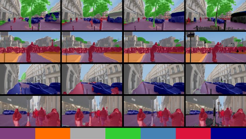
like edge computing [23–25] that place the remote machine close to the edge devices lessen these
barriers, but do not eliminate them and incur additional infrastructure and maintenance costs.
In this paper we propose Adaptive Model Streaming (AMS), a new design paradigm for real-time
video inference on edge devices. AMS uses a remote server to continually adapt a lightweight model
running on the edge device to boost its accuracy for the particular video in real time. The edge
device sends sample video frames to the remote server, which uses them to fine-tune a copy of the
edge device’s model to mimic a large, expensive model via supervised knowledge distillation [26].
The server periodically sends (or “streams”) the updated lightweight model to the edge device for
inference. The insight underlying AMS is that lightweight models perform poorly because they
lack the capacity to learn an accurate model over a wide variety of video frames. By exploiting
the temporal locality in video frames and adapting the model frequently (e.g., every 10 seconds),
AMS overcomes the challenges associated with the low capacity of mobile-friendly models. AMS
also avoids the drawbacks of remote inference approaches. It requires much less bandwidth to send
training samples to the server (e.g., one frame per second) than to send the entire video, and network
delay or outages do not affect the inference latency since inference takes place locally on the device.
We present a design that addresses two main challenges with realizing AMS in practice. First, in
order for AMS to respond to the changes in the video quickly, we need fast adaptation algorithms at
the server. We use a simple online gradient descent approach that continually adapts the model at the
server based on recent samples from a suitably chosen time horizon. Second, we develop techniques
to reduce the downlink and uplink bandwidth requirements for AMS. In the downlink, naïvely
streaming a small semantic segmentation model with 2 million (float16) parameters every 10 seconds
would require over 3 Mbps of bandwidth. Our design uses coordinate descent [27, 28] to train and
send a small fraction of the model parameters in each update. We show that dynamically selecting 5%
of the parameters to send based on gradient signals reduces the downlink bandwidth to only 230 Kbps
with negligible loss in performance. In the uplink, we use standard H.264 video encoding [29]
to compress and upload the training samples to the server every few seconds, requiring a modest
100–400 Kbps. To put AMS’s bandwidth requirement in perspective, it is less than the YouTube
recommended bitrate range of 300–700 Kbps to live stream video at the lowest 240p resolution [30].
We evaluate our approach for real-time semantic segmentation on a Samsung Galaxy S10+
phone (with Adreno 640 GPU) using 7 real-world videos that span a variety of outdoor scenar-
ios, including fixed cameras and moving cameras at walking, running, and driving speeds. Compared
to a lightweight model (DeeplabV3 with MobileNetV2 [11] backbone) pretrained on the Cityscapes
dataset [16] without video-specific customization, AMS provides a 5.1–17.0% boost (10.8% on
average) in mIoU metric (computed relative to the labels from a state-of-the-art DeeplabV3 with
Xception65 [14] backbone model) depending on the video. Also, compared to an approach that
customized the model once for each video based on the first 60 seconds, AMS improves mIoU by
0.1–15.5% (6.5% on average). Figure 1 shows four visual examples comparing the performance of
these on-device approaches to a large, state-of-the-art model. We will release our code and video
datasets at https://github.com/modelstreaming/ams.

2   Related Work

Real-time On-Device Inference. Lightweight mobile-friendly models have been designed both
manually [11] and using neural architecture search techniques [31, 32]. Model quantization and
weight pruning techniques [33–36] have further been shown to reduce the computation footprint of
such models with a small loss in accuracy. Specific to video, some techniques amortize the inference
cost by using optical flow methods to skip inference for some frames [37–39]. Despite the significant
progress made with these optimization techniques, there remains a large gap in the performance of
lightweight models and state-of-the-art solutions. AMS is complementary to on-device optimization
techniques and would also benefit from them. Several proposals offload all or part of the computation
to a powerful remote machine [40–42, 18–20], but these schemes generally require high network
bandwidth, incur higher latency, and are susceptible to network outages [21, 19].
Model Adaptation. Our work is closely related to online learning [43] algorithms for minimizing
dynamic or tracking regret [44–46]. Dynamic regret compares the performance of an online learner
to a sequence of optimal solutions. In our case, the goal is to track the performance of the best
lightweight model at each point in a video. Dynamic regret problems have lower bounds that relate

                                                  2
Real-Time Lightweight Model for the Edge
State-of-the-Art Large Model
(DeepLabV3 with MobileNetV2 backbone)
(DeepLabV3 with
Xception65 backbone)
No Customization One-Time Customization Adaptive Model Streaming (Ours)
Road Sidewalk Building Vegetation Sky Person Car
Figure 1: Semantic segmentation results on real-world outdoor videos: columns from left to right represent
No Customization, One-Time Customization, and AMS. For reference, the results for a large, expensive model
are shown in the last column. AMS provides better accuracy and reduces artifacts (e.g., see the sidewalk detected
in error by the no/one-time customized models in the second row). Notice that the large model (trained on
Cityscapes) also makes some mistakes on these real-world videos. Since AMS aims to mimic the large model
via continual knowledge distillation, its accuracy will improve with a better large model.
regret to a measure of complexity of the optimal sequence of decisions, for example, how quickly the
best model parameters change with time [44]. As video scenes change slowly, it is plausible that the
best models also change gradually in time and online learning can be effective. Several theoretical
works have studied online gradient descent algorithms in this setting with different assumptions
about the loss functions [47, 48]. Other work has focused on the “experts” setting [49–51], where the
learner maintains multiple models and uses the best of them at each time. Our approach is based on
online gradient descent because tracking multiple models per video at a server is expensive.
Other paradigms for model adaptation include lifelong/continual learning [52], meta-learning [53, 54],
federated learning [55], and unsupervised domain adaptation [56, 57]. As our work is only tangentially
related to these efforts, we defer their discussion to Appendix B.
Distillation for Video. Distillation [26] has been proposed as a way to accelerate video inference
for a large corpus of videos [58, 59]. Noscope [58] trains small models for specific tasks (e.g.,
detecting a few object classes) on specific videos offline. JITNet [59] uses online distillation to
specialize a model on video frames as they arrive. The key difference between these works and ours
is that they perform training and inference on the same machine (e.g., server GPU) and the goal
is to speed up inference, whereas in AMS, the student model runs at a low-powered edge device
in real time, but it is trained online at a remote server with sufficient compute power. In particular,
AMS is constrained by limited bandwidth between the edge device and remote server, and crucially
uses coordinate-descent-based [27] training for model distillation to significantly reduce bandwidth
requirements.
3 How Online Adaptation Boosts Performance of Lightweight Models
AMS improves the performance of a lightweight model at an edge device through continual online
adaptation. To gain intuition for how online adaptation improves model performance, we discuss a
simple illustrative example in this section.
3y(t) small τ 0 large τ 0 y(t) small τ 0 large τ 0
1 1 1
f (x) 0.5 0.5 0.5
0 0 0
−0.5 −0.5 −0.5
−1 −1 −1
−1 −0.5 0 0.5 1 0 0.1 0.2 0 0.1 0.2
x t t
(a) labeling function (b) small model (c) large model
Figure 2: A simple example illustrating the importance of considering the model complexity in training horizon.
Let X denote the set of possible input values (e.g., frames in a video). We are given a time-varying
input sequence x(t) ∈ X and must predict an output y(t) ∈ Y given by a deterministic function of
the input: y(t) = f (x(t)). In video semantic segmentation, for example, y(t) corresponds to the
segmentation of the frame x(t). time into a sequence of steps of length τ seconds. Step
Let us divide
n refers to the time interval nτ, nτ + τ . We refer to τ as the inference horizon. At the beginning
of each step n, we pick a set of model parameters wn ∈ Rd to use for prediction during step n. As a
PN
result, we incur a loss of Ln (wn ). The goal is to minimize the total loss over time: n=1 Ln (wn ).
Consider a scalar regression task where X = Y = [−1, 1], and the function f (·) is as shown in Fig. 2a.
Suppose x(t) is a periodic function of time t, which consists of repeated triangles of unit period,
i.e. x(t) = 1 − 2|t − 0.5| for t ∈ [0, 1] defines one period of x(t). As time progresses, x(t) moves
back and forth linearly between -1 and 1. Notice that the characteristics of f (·) change significantly
over its domain [−1, 1]. However, the regression task exhibits temporal locality: since x(t) changes
gradually over time, the regression problem is similar in nearby time intervals. Video inference
exhibits a similar temporal locality because the scenes in a video usually change gradually over time.
Suppose we wish to use polynomials of some degree d to make predictions at each time step. A
natural way to exploit temporal locality is to train the model using recent data at each time step.
Let us define the training horizon as the amount of time into the past used to make a decision and
denote it by τ 0 . For step
n, the online learner fits a polynomial of degree d to (x(t), y(t)) observed
overt ∈ nτ − τ 0 , nτ with Mean-Squared-Error loss, and it uses this model to make predictions in
t ∈ nτ, nτ + τ . We plot y(t) and its predictions for a small linear model (d = 1) and a much larger
polynomial model (d = 50) in Fig. 2b and Fig. 2c, respectively. For each model, we trained two
variants, using small (τ 0 = 1/64) and large (τ 0 = 1/2) values for the training horizon. As these plots
show, the linear model does not have the capacity to fit the data over a long time horizon. However,
by continually adapting the model based on a small training horizon, it is able to make much better
predictions. On the other hand, a high-capacity model does not need to be constrained to a short time
horizon, and in fact it overfits and has poor accuracy when trained with a small horizon.
This example illustrates the importance of picking a training horizon that is well-matched to the
model capacity. Smaller models benefit from a shorter training horizon, i.e. more localized cus-
tomization over time. We will see that for tasks such as video semantic segmentation, such localized
customization of lightweight models can provide a significant boost in accuracy.
4 Cloud-Assisted Adaptive Model Streaming for Real-time Video Inference
In this section we describe the design of a practical real-time video inference system that leverages
adaptive model streaming. Our goal is to continually adapt a lightweight model for a complex task
like video semantic segmentation. Since training on the edge devices is too expensive, we use a cloud
server. Each edge device periodically samples video frames and sends them to the cloud server every
τ seconds. The server uses these frames to train a copy of the edge device’s model using supervised
knowledge distillation [26], and sends the updated model to the edge device. Algorithm 1 shows the
procedure at the server when it is serving a single edge device (we discuss multiple edge devices in
§4.1). The AMS algorithm at the server has two phases: inference and training.
4Inference Phase. To train, the server first needs to label the incoming video frames. It obtains
these labels using a state-of-the-art segmentation model like DeeplabV3 [2] with Xception65 [14]
backbone, which is too large to run at the edge. This model acts as a “teacher” for supervised
knowledge distillation [26]. As the server receives new sample frames, it runs the teacher model on
them to obtain the labels and adds the frames, labels, and frame timestamps to a training data buffer B.
The training phase uses the labeled frames to train the “student” model that runs on the edge device.
Training Phase. As discussed in §3, at the beginning of each step n, we desire a set of model
parameters wn that minimizes the loss of that step Ln (·). The loss Ln (·) depends on the future video
at step n and is unknown. Therefore we train using the cross-entropy loss over sample frames from
the last τ 0 seconds of video. As discussed in §3, choosing a good training horizon directly affects the
performance of online adaptation: a large value of τ 0 could make the data distribution too complex for
a lightweight model, but too small a τ 0 can also cause the model to overfit. The optimal value of τ 0
depends on the model complexity, and the nature of scene changes in the video (e.g., a fast-changing
video may benefit from a shorter τ 0 ). As our results will show, we observed that a training horizon of
about three to five minutes works well across a wide range of videos for video semantic segmentation
using models based on DeeplabV3 with MobileNetV2 [11] backbone and we set τ 0 to four minutes
in our system. To reduce the bandwidth requirement for model streaming (see §4.1), we employ
coordinate descent [27, 28], in which we train a subset of parameters at each training phase and send
only those parameters to the edge device. Specifically, for each training phase, we select a subset of
parameter indices, In , and only update those parameters using the Adam optimizer [60]. We explored
several strategies to select In , as described in detail in §5.3. We found that the Gradient-Guided
strategy achieves the best accuracy. In this strategy, In includes the parameters that the optimizer
estimates to have the largest impact on the loss function. Appendix C describes this method in detail.
Algorithm 1 Adaptive Model Streaming (Server)
1: Initialize the student model with pre-trained parameters w0
2: Send w0 and the student model architecture for the edge device
3: B ← Initialize a time-stamped buffer to store (sample frame, teacher prediction) tuples
4: for n ∈ {1, 2, ...} do
5: Wait until t ≥ nτ
6: Rn ← Set of new sample frames from the edge device . Entering Inference Phase
7: for x ∈ Rn do
8: ỹ ← Use the teacher model to infer the label of x
9: Add (x, ỹ) to B with time stamp of receiving x
10: end for
11: In ← Select a subset of model parameter indices . Entering Training Phase
12: for k ∈ {1, 2, ..., K} do
13: Sk ← Uniformly sample a mini-batch of data points from B over the last τ 0 seconds
14: Candidate updates ← Calculate Adam optimizer updates w.r.t the empirical loss on Sk
15: Apply candidate updates to model parameters indexed by In
16: end for
17: w̃n ← New value of model parameters which are indexed by In
18: Send (w̃n , In ) for the edge device
19: end for
4.1 Practical Challenges
Reducing Downlink Bandwidth Requirements. Naïvely streaming a large model to the edge
device can consume a significant amount of bandwidth. For example, sending a relatively simple
model with 2 million parameters every 10 seconds would require 3.2 Mbps of downlink bandwidth.
In our experiments, using coordinate descent with a Gradient-Guided strategy to send 5% of the
parameters in each model update reduces the required bandwidth by 14× with negligible loss in
performance compared to updating the complete model. Along with the updated parameters, w̃n ,
we must also send their location in the model, In , which introduces additional bandwidth overhead.
A simple strategy is to send a bit-vector identifying the location of the parameters with each model
update. As the bit-vector is sparse, it can be compressed and we use gzip [61] in our experiments to
5carry this out. Further bandwidth reductions could be achieved using standard model compression
and quantization techniques [33, 34, 36].
Reducing Uplink Bandwidth Requirements. To reduce the uplink bandwidth, the edge device
does not send sampled frames immediately. Instead it buffers samples corresponding to τ seconds
of video (e.g., τ = 10), and it runs H.264 [29] video encoding on this buffer to compress it before
transmission. The time taken at the edge device to fill the compression buffer and transmit a new batch
of samples is hidden from the server by overlapping it with the training phase of the previous step.
By synchronizing the transmission of new data with the start of the inference phase, we minimize the
staleness of the training data at the server.
Maximizing Server Utilization. Running a GPU in the cloud, e.g., NVIDIA Tesla V100, currently
costs at least $1 per hour. Hence, it is important to serve multiple edge devices per GPU to keep
per-user cost low. Every user that joins a cloud server requires its own share of GPU resources
for inference and training operations. In our prototype, we use a simple strategy that iterates in a
round-robin fashion across multiple video sessions, completing one inference and training step per
session. By allowing only one process to access the GPU at a time, we minimize context switching
overhead. Our results show that this technique is effective and can support model streaming for up to
seven video sessions per an NVIDIA Tesla V100 GPU with negligible loss in performance.
5 Evaluation
5.1 Methodology
We evaluate AMS on the task of semantic segmentation using the DeeplabV3 [2] class of models.
These models have a wide range of sizes but share the same architectural ideas. As the initial model,
we start with models pre-trained on the Cityscapes [16] semantic segmentation dataset. These models
themselves include a backbone pre-trained on Imagenet and MS-COCO [62, 63]. On the edge
device, we use the model with MobileNetV2 [11] backbone at an input image resolution of 512×256,
which runs smoothly in real-time at 30 frame-per-second (fps) on a Samsung Galaxy S10+ phone’s
Adreno 640 GPU with less than 40 ms camera-to-label latency. We compare the following schemes:
• No Customization: We run the pre-trained model without video-specific customization.
• One-Time Customization: We collect training samples at four frames per second during the first
60 seconds of the video, fine-tune the entire model on these samples at the server and send it to the
edge. This adaptation happens only once for every video. Comparing this scheme with AMS will
show the benefit of continuous adaptation.
• AMS: We use Algorithm 1 at the server with τ = 10 sec, τ 0 = 250 sec, and K = 20 iterations.
Unless otherwise stated, 5% of the model parameters are selected using the Gradient-Guided
strategy. We use a single NVIDIA Tesla V100 GPU for both training and inference at the server.
One-Time Customization and AMS use DeeplabV3 with Xception65 [14] backbone pre-trained on
Cityscapes as the teacher model. In both schemes, edge devices transmit sample frames at a resolution
of 1024×512 to the cloud server after compression, as described in §4.1. The server upscales the
received frames to a resolution of 1800×900 before labeling them with the teacher. For all training
purposes, we use Adam optimizer [60] with a learning rate of 0.001, β1 = 0.9, β2 = 0.999.
Videos. We use 7 diverse videos chosen from YouTube with a length of 7–15 minutes for evaluation.
Since our semantic segmentation models were trained on Cityscapes driving scenes, we consider
videos of outdoor scenes for which our best model with Xception65 backbone has good visual
performance. However, the videos cover a range of scene variability, representing different scenarios
of interest including fixed cameras and moving cameras at walking, running, and driving speeds.
Table 4 and Fig. 5 in Appendix A provide a description of the videos and some examples of scenes.
Metric. To evaluate the accuracy of different schemes, we collect the inferred labels on the edge
device and compare them against labels extracted for the same video frames using a state-of-the-art
DeeplabV3 with Xception65 backbone model (pre-trained on Cityscapes) running at full resolu-
tion (2048×1024) offline. We report the mean Intersection-over-Union (miou) metric relative to the
labels produced by this reference model. The metric computes the Intersection-over-Union (defined
as the number of true positives divided by the sum of true positives, false negatives and false positives)
6Table 1: Comparison of mIoU (in percent) for different methods across 7 evaluation videos.
Vid1 Vid2 Vid3 Vid4 Vid5 Vid6 Vid7
No Customization 71.91 54.48 72.80 69.93 49.04 66.26 61.31
One-Time Customization 88.45 55.99 83.55 69.53 55.12 65.07 58.12
AMS (5% of parameters) 88.55 71.45 85.36 75.53 59.49 71.40 69.44
Table 2: AMS bandwidth usage (in Kbps) and mIoU (in percent) for updating different fraction of model
parameters using the Gradient-Guided strategy.
Fraction BW(Kbps) Vid1 Vid2 Vid3 Vid4 Vid5 Vid6 Vid7
100% 3302 89.49 72.97 85.90 75.83 60.24 71.15 70.69
20% 812 88.91 72.83 85.52 76.38 59.65 72.56 70.57
10% 435 88.61 72.13 85.46 76.16 60.18 71.98 70.11
5% 230 88.55 71.45 85.36 75.53 59.49 71.40 69.44
1% 51.8 84.59 68.37 84.41 73.95 57.53 69.27 68.16
for each class, and takes a mean over the classes. We manually select a subset of most populous
Cityscapes output classes in each of these videos as summarized in Table 4 in Appendix A.
5.2 Results
Comparison to baselines. Table 1 summarizes the results. The No Customization model has the
worst accuracy among these three methods which is 5.1–17.0% (10.8% on average) below AMS.
The One-Time Customization model performs better as it is specialized for each video using the
initial frames. However, since a video itself can vary significantly over time, AMS performs even
better by continually adapting the model to the video. AMS outperforms One-Time Customization
by 0.1–15.5% (6.5% on average) across the 7 videos. It achieves the highest improvement in Vid2
due to its high scene variability (comedian performing, crowd watching, streets, etc.), which makes
continuous adaptation crucial. The smallest improvement is in Vid1, a stationary interview scene, for
which One-Time Customization performs well.
Accuracy vs. bandwidth usage. Table 2 shows the accuracy and downlink bandwidth usage for
sending different fractions of the student model to the device on each update. We observe that
coordinate descent is very effective. Sending only 5% of the model parameters results in only 0.76%
loss of accuracy on average across the 7 videos, but it reduces the downlink bandwidth requirement
significantly, from 3.3 Mbps to update the full model (∼2 million parameters) to 230 Kbps. In the
uplink, our method of compressing the sampled frames before sending to the cloud server (§4.1)
requires a modest bandwidth of 100–400 Kbps (on different videos). The loss in accuracy caused by
this compression is negligible (0.07% on average across the videos).
Supporting multiple clients with one server. In Fig. 3 we show the decrease (w.r.t. single client) in
average mIoU when different number of clients share a GPU in round-robin manner. We observe that
even with this simple scheduling algorithm, AMS scales to up to 7 clients on a single V100 GPU
with less than 1% loss in mIoU. As we see later in the results, there is room for supporting even more
clients per GPU by prioritizing certain videos that need more frequent model updates over others.
5.3 Impact of Design Choices
Coordinate Descent Strategy. Table 3 compares the Gradient-Guided strategy with four baselines
for subset parameters selection in the training phase. In the First, Last, and First&Last strategies,
the subset parameters are from the initial layers, final layers, and an equal split of both, respec-
tively. The Random strategy samples parameters uniformly from the entire network. We compare
these strategies on their reduction in accuracy relative to sending full model updates. We observe
that the Gradient-Guided performs best, followed by Random. Random is notably worse than
Gradient-Guided when training a very small fraction (1%) of model parameters. The methods that
update only the first or last model layers are substantially worse than the other approaches.
Training Horizon. As explained using the simple example in §3, the ideal training horizon, τ 0 ,
depends on the model capacity, with smaller models expected to perform better when trained on
7Table 3: Difference in accuracy relative to full-model training (in percent) averaged over the 7 evaluation videos
for different coordinate descent strategies.
Fraction Gradient-Guided Last First First&Last Random
20% +0.14 -5.43 -2.34 -0.82 -0.03
10% -0.26 -6.13 -4.89 -1.96 -0.44
5% -0.76 -7.95 -7.16 -2.64 -1.21
1% -2.49 -9.97 -14.44 -6.61 -4.39
Default 2x Smaller Vid1 Vid4 Vid5
0
∆ mIoU (%)
66
mIoU (%)
mIoU (%)
63 80
−1
60
60
−2
57
2 4 6 8 10 100 200 300 400 500 100 101 102 103
0
Number of clients Training horizon (τ ) in sec Update interval (τ ) in sec
Figure 3: Average multiclient (a) (b)
mIoU degradation compared to Figure 4: Impact of training horizon and training frequency on AMS
single-client performance. Semantic Segmentation task.
shorter time horizons. We evaluate this intuition for the video semantic segmentation task. We
consider two variations of the student model: (i) the default DeeplabV3 with MobileNetV2 backbone,
(ii) a smaller version with the same architecture but with half the number of channels in each
convolutional layer. We pick 50 points in time uniformly distributed over the course of one video
(Vid6). For each time t, we train the two student models on the frames in the interval [t − τ 0 , t)
and then evaluate them on frames in [t, t + τ ) (with τ = 16 sec). We plot the average accuracy
of the two variants for each value of the training horizon τ 0 in Fig. 4a. As expected, the smaller
model’s accuracy peaks at some training horizon (τ 0 ≈ 250 sec) and degrades with larger τ 0 as the
model capacity is insufficient to learn wider variations in the training data. The default student model
exhibits the same behavior, but with a more gradual drop for large τ 0 . Overall we found that a training
horizon of 200–400 seconds generally works well across all of the videos in our dataset.
Model Update Frequency. The frequency of model updates dictates how long a particular model
is used at the edge device. Intuitively, more frequent updates should lead to better accuracy, at the
cost of higher bandwidth and server computation. To evaluate the impact of model update frequency,
we measure the accuracy for three videos, with different update intervals τ ranging from 1 to 1000
seconds and a training horizon τ 0 of 256 seconds. Figure 4b shows the results. As expected, a smaller
τ improves performance, but the impact of slower model updates varies across the three videos. For
example, rapid model updates barely improve Vid1, which is an interview with a stationary scene.
However, the effect is visible for Vid4 and Vid5 as they are walking scenes. This suggests that we can
support more video sessions per GPU by prioritizing videos that need more frequent model updates.
Frame Sampling Rate. Table 5 in Appendix D shows the impact of varying the frame sampling rate
on accuracy for 3 videos. Sampling faster than 1 frame-per-second provides negligible improvement
in accuracy along increasing bandwidth usage. As these results suggest, the sampling rate can also be
reduced at the cost of a small reduction in accuracy.
6 Conclusion
We presented an approach for improving the performance of real-time video inference on low-powered
edge devices that uses a remote server to continually train and stream model updates to the edge
device at a time scale of 10–100 seconds. Further, we proposed techniques to reduce the network
bandwidth requirements of adaptive model streaming to levels easily sustainable on today’s wireless
networks. Extensive evaluation of AMS on a wide range of videos showed a rise of 5.1–17.0% in
mIoU scores on the task of real-time semantic segmentation using a mobile GPU, which can be a
significant improvement for the quality of real-time video inference on edge devices.
8Broader Impact
Real-time video inference on edge devices, which our work aims to make practical, has a wide range
of societal applications. Examples include tasks like semantic segmentation in autonomous driving,
visual tracking and object recognition in drone navigation, infrastructure monitoring using drones,
super-resolution in video streaming, object detection on home devices like robotic vacuums, and
future research on enabling augmented reality with neural networks. Real-time video inference also
has potential negative applications, such as privacy-violating surveillance, and real-time “deepfake”
models used to impersonate others on video calls. Failure of the system can result in poor inference
accuracy, with consequences that depend on the application. Like systems that rely on remote
inference, our system is vulnerable to abuse by a malicious and untrusted server, since clients must
stream video to a remote server for training.
References
[1] Joseph Redmon, Santosh Divvala, Ross Girshick, and Ali Farhadi. You only look once: Unified,
real-time object detection. In Proceedings of the IEEE conference on computer vision and
pattern recognition, pages 779–788, 2016.
[2] Liang-Chieh Chen, George Papandreou, Iasonas Kokkinos, Kevin Murphy, and Alan L. Yuille.
Deeplab: Semantic image segmentation with deep convolutional nets, atrous convolution, and
fully connected crfs. IEEE Transactions on Pattern Analysis and Machine Intelligence, 40:
834–848, 2018.
[3] Zhe Cao, Tomas Simon, Shih-En Wei, and Yaser Sheikh. Realtime multi-person 2d pose
estimation using part affinity fields. In Proceedings of the IEEE Conference on Computer Vision
and Pattern Recognition, pages 7291–7299, 2017.
[4] Tensorflow. Deelab semantic segmentation model zoo. https://github.com/tensorflow/
models/blob/master/research/deeplab/g3doc/model_zoo.md, 2020.
[5] Tensorflow. Tensorflow object detection model zoo. https://github.com/tensorflow/
models/blob/master/research/object_detection/g3doc/detection_model_zoo.
md, 2020.
[6] Coral Edge TPU datasheet. https://coral.ai/docs/dev-board/datasheet/, 2020.
[7] NVIDIA Jetson Nano datasheet. https://developer.nvidia.com/embedded/
jetson-nano, 2020.
[8] Edge TPU performance benchmarks. https://coral.ai/docs/edgetpu/benchmarks/,
2020.
[9] Junjue Wang, Ziqiang Feng, Zhuo Chen, Shilpa George, Mihir Bala, Padmanabhan Pillai,
Shao-Wen Yang, and Mahadev Satyanarayanan. Bandwidth-efficient live video analytics for
drones via edge computing. pages 159–173, 10 2018. doi: 10.1109/SEC.2018.00019.
[10] Qianlin Liang, Prashant J. Shenoy, and David Irwin. AI on the Edge: Rethinking AI-based IoT
Applications Using Specialized Edge Architectures. ArXiv, abs/2003.12488, 2020.
[11] Mark Sandler, Andrew G. Howard, Menglong Zhu, Andrey Zhmoginov, and Liang-Chieh
Chen. Mobilenetv2: Inverted residuals and linear bottlenecks. 2018 IEEE/CVF Conference on
Computer Vision and Pattern Recognition, pages 4510–4520, 2018.
[12] Andrew Howard, Mark Sandler, Grace Chu, Liang-Chieh Chen, Bo Chen, Mingxing Tan,
Weijun Wang, Yukun Zhu, Ruoming Pang, Vijay Vasudevan, Quoc V. Le, and Hartwig Adam.
Searching for mobilenetv3. 2019 IEEE/CVF International Conference on Computer Vision
(ICCV), pages 1314–1324, 2019.
[13] M. Tan, B. Chen, R. Pang, V. Vasudevan, M. Sandler, A. Howard, and Q. V. Le. Mnasnet:
Platform-aware neural architecture search for mobile. In 2019 IEEE/CVF Conference on
Computer Vision and Pattern Recognition (CVPR), pages 2815–2823, 2019.
9[14] F. Chollet. Xception: Deep learning with depthwise separable convolutions. In 2017 IEEE
Conference on Computer Vision and Pattern Recognition (CVPR), pages 1800–1807, 2017.
[15] Mark Everingham, S. Eslami, Luc Van Gool, Christopher Williams, John Winn, and Andrew
Zisserman. The pascal visual object classes challenge: A retrospective. International Journal
of Computer Vision, 111, 01 2014. doi: 10.1007/s11263-014-0733-5.
[16] Marius Cordts, Mohamed Omran, Sebastian Ramos, Timo Rehfeld, Markus Enzweiler, Rodrigo
Benenson, Uwe Franke, Stefan Roth, and Bernt Schiele. The cityscapes dataset for semantic
urban scene understanding. 2016 IEEE Conference on Computer Vision and Pattern Recognition
(CVPR), pages 3213–3223, 2016.
[17] Xianzhi Du, Tsung-Yi Lin, Pengchong Jin, Golnaz Ghiasi, Mingxing Tan, Yin Cui, Quoc V
Le, and Xiaodan Song. Spinenet: Learning scale-permuted backbone for recognition and
localization. arXiv preprint arXiv:1912.05027, 2019.
[18] Christopher Olston, Noah Fiedel, Kiril Gorovoy, Jeremiah Harmsen, Li Lao, Fangwei Li,
Vinu Rajashekhar, Sukriti Ramesh, and Jordan Soyke. Tensorflow-serving: Flexible, high-
performance ml serving. arXiv preprint arXiv:1712.06139, 2017.
[19] Daniel Crankshaw, Xin Wang, Guilio Zhou, Michael J Franklin, Joseph E Gonzalez, and Ion
Stoica. Clipper: A low-latency online prediction serving system. In 14th {USENIX} Symposium
on Networked Systems Design and Implementation ({NSDI} 17), pages 613–627, 2017.
[20] Chengliang Zhang, Minchen Yu, Wei Wang, and Feng Yan. Mark: Exploiting cloud services
for cost-effective, slo-aware machine learning inference serving. In 2019 {USENIX} Annual
Technical Conference ({USENIX} {ATC} 19), pages 1049–1062, 2019.
[21] Sadjad Fouladi, John Emmons, Emre Orbay, Catherine Wu, Riad S Wahby, and Keith Win-
stein. Salsify: Low-latency network video through tighter integration between a video codec
and a transport protocol. In 15th {USENIX} Symposium on Networked Systems Design and
Implementation ({NSDI} 18), pages 267–282, 2018.
[22] Keith Winstein, Anirudh Sivaraman, and Hari Balakrishnan. Stochastic forecasts achieve high
throughput and low delay over cellular networks. In Presented as part of the 10th {USENIX}
Symposium on Networked Systems Design and Implementation ({NSDI} 13), pages 459–471,
2013.
[23] W. Shi, J. Cao, Q. Zhang, Y. Li, and L. Xu. Edge computing: Vision and challenges. IEEE
Internet of Things Journal, 3(5):637–646, 2016.
[24] Pedro Garcia Lopez, Alberto Montresor, Dick Epema, Anwitaman Datta, Teruo Higashino,
Adriana Iamnitchi, Marinho Barcellos, Pascal Felber, and Etienne Riviere. Edge-centric
computing: Vision and challenges. SIGCOMM Comput. Commun. Rev., 45(5):37–42, September
2015. ISSN 0146-4833. doi: 10.1145/2831347.2831354. URL https://doi.org/10.1145/
2831347.2831354.
[25] Flavio Bonomi, Rodolfo Milito, Jiang Zhu, and Sateesh Addepalli. Fog computing and its
role in the internet of things. In Proceedings of the First Edition of the MCC Workshop on
Mobile Cloud Computing, MCC ’12, page 13–16, New York, NY, USA, 2012. Association
for Computing Machinery. ISBN 9781450315197. doi: 10.1145/2342509.2342513. URL
https://doi.org/10.1145/2342509.2342513.
[26] Geoffrey Hinton, Oriol Vinyals, and Jeff Dean. Distilling the knowledge in a neural network.
arXiv preprint arXiv:1503.02531, 2015.
[27] Stephen J. Wright. Coordinate descent algorithms. Mathematical Programming, 151:3–34,
2015.
[28] Yurii NESTEROV. Efficiency of coordinate descent methods on huge-scale optimization
problems. Université catholique de Louvain, Center for Operations Research and Econometrics
(CORE), CORE Discussion Papers, 22, 01 2010. doi: 10.1137/100802001.
10[29] T. Wiegand, G. J. Sullivan, G. Bjontegaard, and A. Luthra. Overview of the h.264/avc video
coding standard. IEEE Transactions on Circuits and Systems for Video Technology, 13(7):
560–576, 2003.
[30] Choose live encoder settings, bitrates, and resolutions. https://support.google.com/
youtube/answer/2853702?hl=en. Accessed: 2020-06-01.
[31] Barret Zoph and Quoc V Le. Neural architecture search with reinforcement learning. arXiv
preprint arXiv:1611.01578, 2016.
[32] Bichen Wu, Xiaoliang Dai, Peizhao Zhang, Yanghan Wang, Fei Sun, Yiming Wu, Yuandong
Tian, Peter Vajda, Yangqing Jia, and Kurt Keutzer. Fbnet: Hardware-aware efficient convnet
design via differentiable neural architecture search. In Proceedings of the IEEE Conference on
Computer Vision and Pattern Recognition, pages 10734–10742, 2019.
[33] Yihui He, Ji Lin, Zhijian Liu, Hanrui Wang, Li-Jia Li, and Song Han. Amc: Automl for model
compression and acceleration on mobile devices. In Proceedings of the European Conference
on Computer Vision (ECCV), pages 784–800, 2018.
[34] Darryl Lin, Sachin Talathi, and Sreekanth Annapureddy. Fixed point quantization of deep
convolutional networks. In International Conference on Machine Learning, pages 2849–2858,
2016.
[35] Davis Blalock, Jose Javier Gonzalez Ortiz, Jonathan Frankle, and John Guttag. What is the
state of neural network pruning? arXiv preprint arXiv:2003.03033, 2020.
[36] Yu Cheng, Duo Wang, Pan Zhou, and Tao Zhang. A survey of model compression and
acceleration for deep neural networks. ArXiv, abs/1710.09282, 2017.
[37] Zheng Zhu, Qiang Wang, Bo Li, Wei Wu, Junjie Yan, and Weiming Hu. Distractor-aware
siamese networks for visual object tracking. In Proceedings of the European Conference on
Computer Vision (ECCV), pages 101–117, 2018.
[38] Xizhou Zhu, Yuwen Xiong, Jifeng Dai, Lu Yuan, and Yichen Wei. Deep feature flow for
video recognition. In Proceedings of the IEEE Conference on Computer Vision and Pattern
Recognition, pages 2349–2358, 2017.
[39] Yuan-Ting Hu, Jia-Bin Huang, and Alexander Schwing. Maskrnn: Instance level video object
segmentation. In Advances in neural information processing systems, pages 325–334, 2017.
[40] Yiping Kang, Johann Hauswald, Cao Gao, Austin Rovinski, Trevor Mudge, Jason Mars, and
Lingjia Tang. Neurosurgeon: Collaborative intelligence between the cloud and mobile edge.
ACM SIGARCH Computer Architecture News, 45(1):615–629, 2017.
[41] Sandeep P Chinchali, Eyal Cidon, Evgenya Pergament, Tianshu Chu, and Sachin Katti. Neural
networks meet physical networks: Distributed inference between edge devices and the cloud. In
Proceedings of the 17th ACM Workshop on Hot Topics in Networks, pages 50–56, 2018.
[42] Sandeep Chinchali, Apoorva Sharma, James Harrison, Amine Elhafsi, Daniel Kang, Evgenya
Pergament, Eyal Cidon, Sachin Katti, and Marco Pavone. Network offloading policies for cloud
robotics: a learning-based approach. arXiv preprint arXiv:1902.05703, 2019.
[43] Shai Shalev-Shwartz et al. Online learning and online convex optimization. Foundations and
Trends R in Machine Learning, 4(2):107–194, 2012.
[44] Eric C Hall and Rebecca M Willett. Dynamical models and tracking regret in online convex
programming. In Proceedings of the 30th International Conference on International Conference
on Machine Learning-Volume 28, pages I–579, 2013.
[45] Lijun Zhang, Shiyin Lu, and Zhi-Hua Zhou. Adaptive online learning in dynamic environments.
In Advances in neural information processing systems, pages 1323–1333, 2018.
[46] Aryan Mokhtari, Shahin Shahrampour, Ali Jadbabaie, and Alejandro Ribeiro. Online optimiza-
tion in dynamic environments: Improved regret rates for strongly convex problems. In 2016
IEEE 55th Conference on Decision and Control (CDC), pages 7195–7201. IEEE, 2016.
11[47] Martin Zinkevich. Online convex programming and generalized infinitesimal gradient ascent. In
Proceedings of the 20th international conference on machine learning (icml-03), pages 928–936,
2003.
[48] Elad Hazan, Amit Agarwal, and Satyen Kale. Logarithmic regret algorithms for online convex
optimization. Machine Learning, 69(2-3):169–192, 2007.
[49] Mark Herbster and Manfred K Warmuth. Tracking the best expert. Machine learning, 32(2):
151–178, 1998.
[50] Tianbao Yang, Lijun Zhang, Rong Jin, and Jinfeng Yi. Tracking slowly moving clairvoyant:
optimal dynamic regret of online learning with true and noisy gradient. In Proceedings of the
33rd International Conference on International Conference on Machine Learning-Volume 48,
pages 449–457, 2016.
[51] Elad Hazan and Comandur Seshadhri. Efficient learning algorithms for changing environments.
In Proceedings of the 26th annual international conference on machine learning, pages 393–400,
2009.
[52] David Lopez-Paz and Marc’Aurelio Ranzato. Gradient episodic memory for continual learning.
In Advances in Neural Information Processing Systems, pages 6467–6476, 2017.
[53] Chelsea Finn, Pieter Abbeel, and Sergey Levine. Model-agnostic meta-learning for fast adap-
tation of deep networks. In Proceedings of the 34th International Conference on Machine
Learning-Volume 70, pages 1126–1135. JMLR. org, 2017.
[54] Sachin Ravi and Hugo Larochelle. Optimization as a model for few-shot learning. International
Conference on Learning Representations (ICLR), 2017.
[55] Brendan McMahan, Eider Moore, Daniel Ramage, Seth Hampson, and Blaise Aguera y Arcas.
Communication-efficient learning of deep networks from decentralized data. In Artificial
Intelligence and Statistics, pages 1273–1282, 2017.
[56] Shai Ben-David, John Blitzer, Koby Crammer, and Fernando Pereira. Analysis of representations
for domain adaptation. In Advances in neural information processing systems, pages 137–144,
2007.
[57] Guoliang Kang, Lu Jiang, Yi Yang, and Alexander G Hauptmann. Contrastive adaptation
network for unsupervised domain adaptation. In Proceedings of the IEEE Conference on
Computer Vision and Pattern Recognition, pages 4893–4902, 2019.
[58] Daniel Kang, John Emmons, Firas Abuzaid, Peter Bailis, and Matei Zaharia. Noscope: optimiz-
ing neural network queries over video at scale. arXiv preprint arXiv:1703.02529, 2017.
[59] Ravi Teja Mullapudi, Steven Chen, Keyi Zhang, Deva Ramanan, and Kayvon Fatahalian. Online
model distillation for efficient video inference. In Proceedings of the IEEE International
Conference on Computer Vision, pages 3573–3582, 2019.
[60] Diederik P. Kingma and Jimmy Ba. Adam: A method for stochastic optimization. CoRR,
abs/1412.6980, 2015.
[61] P. Deutsch. Rfc1952: Gzip file format specification version 4.3, 1996.
[62] J. Deng, W. Dong, R. Socher, L. Li, Kai Li, and Li Fei-Fei. Imagenet: A large-scale hierarchical
image database. In 2009 IEEE Conference on Computer Vision and Pattern Recognition, pages
248–255, 2009.
[63] Tsung-Yi Lin, Michael Maire, Serge J. Belongie, James Hays, Pietro Perona, Deva Ramanan,
Piotr Dollár, and C. Lawrence Zitnick. Microsoft coco: Common objects in context. ArXiv,
abs/1405.0312, 2014.
[64] David Rolnick, Arun Ahuja, Jonathan Schwarz, Timothy Lillicrap, and Gregory Wayne. Expe-
rience replay for continual learning. In Advances in Neural Information Processing Systems,
pages 348–358, 2019.
12[65] James Kirkpatrick, Razvan Pascanu, Neil Rabinowitz, Joel Veness, Guillaume Desjardins,
Andrei A Rusu, Kieran Milan, John Quan, Tiago Ramalho, Agnieszka Grabska-Barwinska, et al.
Overcoming catastrophic forgetting in neural networks. Proceedings of the national academy of
sciences, 114(13):3521–3526, 2017.
[66] Michael McCloskey and Neal J Cohen. Catastrophic interference in connectionist networks:
The sequential learning problem. In Psychology of learning and motivation, volume 24, pages
109–165. Elsevier, 1989.
[67] Chelsea Finn, Aravind Rajeswaran, Sham Kakade, and Sergey Levine. Online meta-learning.
arXiv preprint arXiv:1902.08438, 2019.
[68] Keith Bonawitz, Hubert Eichner, Wolfgang Grieskamp, Dzmitry Huba, Alex Ingerman, Vladimir
Ivanov, Chloe Kiddon, Jakub Konecny, Stefano Mazzocchi, H Brendan McMahan, et al. Towards
federated learning at scale: System design. arXiv preprint arXiv:1902.01046, 2019.
[69] Julie Nutini, Mark Schmidt, Issam H. Laradji, Michael Friedlander, and Hoyt Koepke. Co-
ordinate descent converges faster with the gauss-southwell rule than random selection. In
Proceedings of the 32nd International Conference on International Conference on Machine
Learning - Volume 37, ICML’15, page 1632–1641. JMLR.org, 2015.
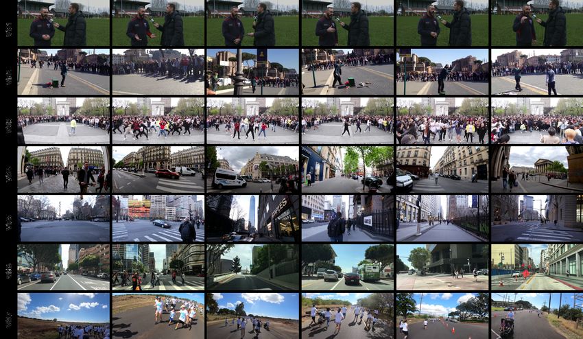
13Appendix A Videos
Our video corpus includes seven publicly available videos from Youtube, with 7–15 minutes in
duration. These videos span different levels of scene variability and were captured with four types of
cameras: Stationary, Phone, Headcam, and DashCam. For each video, we manually select 5–7 classes
that are detected frequently by our best semantic segmentation model (DeeplabV3 with Xception65
backbone trained on Cityscapes data) at full resolution. Table 4 shows summary information about
these videos. In Fig. 5 we show six sample frames for each video. For viewing the raw and labeled
videos, please refer to https://github.com/modelstreaming/ams.
Table 4: Videos description
Tag Description Camera Style Classes
Vid1 Interview with head-coach Stationary Buildings, Vegetation, Terrain, Sky, People, Cars
Vid2 Street comedian in Rome Phone Streets, Sidewalks, Buildings, Vegetation, Sky, People
Vid3 Group dance in a park Stationary Sidewalks, Buildings, Vegetation, Sky, People
Vid4 Street walking in Paris Phone Streets, Buildings, Vegetation, Sky, People, Cars
Vid5 Street walking in NYC Phone Streets, Buildings, Vegetation, Sky, People, Cars
Vid6 Driving in LA 4K DashCam Streets, Sidewalks, Buildings, Vegetation, Sky, People, Cars
Vid7 Bubble run in Honolulu Headcam Streets, Terrain, Vegetation, Sky, Person
Figure 5: Sample video frames.
Appendix B Other Related Work
Continual/Lifelong Learning. The goal of lifelong learning [52] is to accumulate knowledge over
time [64]. Hence the main challenge is to improve the model based on new data over time, while
not forgetting data observed in the past [65, 66]. However, as the lightweight models have limited
capacity, in AMS we aim to track the best model at each point in time, and these models are allowed
not to have the same performance on the old data.
Meta Learning. Meta learning [53, 54, 67] algorithms aim to learn models that can be adapted to
any target task in a set of tasks, given only few samples (shots) from that task. Meta learning is not
a natural framework for continual model specialization for video. First, as videos have temporal
14coherence, there is little benefit in handling an arbitrary order of task arrival. Indeed, it is more natural
to adapt the latest model over time instead of always training from a meta-learned initial model.1
Second, training such a meta model usually requires two nested optimization steps [53], which would
significantly increase the server’s computation overhead. Finally, most meta learning work considers
a finite set of tasks but this notion is not well-suited to video.
Federated Learning. Another body of work on improving edge models over time is federated
learning [55], in which the training mainly happens on the edge devices and device updates are
aggregated at a server. The server then broadcasts the aggregated model back to all devices. Such
updates happen at a time scale of hours to days [68], and they aim to learn better generalizable models
that incorporate data from all edge devices. In contrast, the training in AMS takes place at the server
at a time scale of a couple of seconds and intends to improve the accuracy of an individual edge
device’s model for its particular video.
Unsupervised Adaptation. Domain adaptation methods [56, 57] intend to compensate for shifts
between training and test data distributions. In a typical approach, an unsupervised algorithm fine-
tunes the model over the entire test data at once. However, frame distribution can drift over time. As
our results show, one-time fine-tuning can have a much lower accuracy than continuous adaptation.
However, it is too expensive to provide a fast adaptation (at a timescale of 10–100 seconds) of these
models at the edge, even using unsupervised methods. Moreover, using AMS we benefit from the
superior performance of supervised training by running state-of-the-art models as the “teacher” for
knowledge distillation [26] in the cloud.
Appendix C The Gradient-Guided strategy
To reduce the bandwidth requirement of model streaming, we employ coordinate descent [27] training.
In each training phase, we select a small subset (e.g., 5%) of parameters (coordinates) to update.
We expand the Lines 11–16 in Algorithm 1 by adding the details of Gradient-Guided strategy as in
Algorithm 2.
The pseudo code describes the procedure in the nth training phase. Each training phase includes K
iterations with randomly-sampled mini-batches of data points from the last τ 0 seconds of video. In
training iteration k, we update the first and second moments of the optimizer (mn,k and vn,k ) using
the typical Adam rules (Lines 7–10). We then calculate the Adam updates for all model parameters
un,k (Lines 11–12). However, we only apply the updates for parameters determined by the binary
mask bn (Line 13). Here, bn is a vector of the same size as the model parameters, with ones at
indices that are in In and zeros otherwise. In the Gradient-Guided strategy, we select the In to index
the γ fraction of parameters with the largest absolute value of the vector un−1 . We update un at the
end of each training phase to reflect the latest values of the Adam updates for all parameters (Line
15). In the first training phase, In is selected uniformly at random.
The intuition behind this algorithm is to update the subset of parameters that could provide the largest
improvement in the loss function. A typical way to achieve this would be to update the parameters with
the largest gradient magnitude in each training phase. This is called the Gauss-Southwell selection
rule [69]. Algorithm 2 applies this intuition to coordinate descent using the Adam optimizer [60].
To perform coordinate descent using Adam, we consider the parameters with the largest magnitude
of change in Adam’s parameter update. Adam uses the first and second moments of past gradients
to suggest a less noisy and more robust parameter update than just the gradient for one mini-batch.
Notice, however, that to use this signal, we have to update the moments for all parameters in all
training iterations, regardless of whether or not we actually update those parameters in Line 13.
Appendix D Effect of Sampling Rate
To evaluate the effects of sampling rate, we profiled AMS’s performance for different sampling
rates, ranging from one frame every 10 secs to 30 frames per second (all available frames). In this
experiment, we use a training horizon of τ 0 = 250 seconds and a model update interval of τ = 10
seconds. To minimize the impact of other system design choices, we train the entire model parameters
1
An exception is a video that changes substantially in a short period of time, for example, a camera that
moves between indoor and outdoor environments. In such cases, a meta model may enable faster adaptation.
15Algorithm 2 Gradient-Guided Strategy using Adam Optimizer
1: In ← Indices of γ fraction of largest absolute values in un−1 . Entering nth Training Phase
2: bn ← binary mask of model parameters; 1 iff indexed by In
3: wn,0 ← wn−1 . Use the latest model parameters as the next starting point
4: mn,0 ← mn−1,K . Initialize the first moment estimate to its latest value
5: vn,0 ← vn−1,K . Initialize the second moment estimate to its latest value
6: for k ∈ {1, 2, ..., K} do
7: Sk ← Uniformly sample a mini-batch of data points from B over the last τ 0 seconds
8: gn,k ← ∇w L̃(Sk ; wn,k−1 ) . Get the gradient of all model parameters w.r.t. loss on Sk
9: mn,k ← β1 · mn,k−1 + (1 − β1 ) · gn,k . Update first moment estimate
2
10: vn,k ← β2 · vn,k−1 + (1 − β2 ) · gn,k . Update second moment estimate
11: i←i+1 √ . Increment Adam’s global step count
1−β2i m
12: un,k ← α · 1−β1i
· √ n,k . Calculate the Adam updates for all model parameters
vn,k +
13: wn,k ← wn,k−1 − un,k ∗ bn . Update the parameters indexed by In (∗ is elem.-wise mul.)
14: end for
15: un ← un,K
16: wn ← wn,K
in every update, starting from the pre-trained checkpoint. Table 5 shows the impact of sampling
rate on mIoU across different videos. We observe that there is negligible performance improvement
across all videos in sampling faster than a single frame per second.
Table 5: Impact of training frame sampling rate on mIoU.
Sampling Rate (fps) 30 10 3.3 1 0.33 0.1
Vid1 87.76 87.60 87.78 87.72 87.01 86.31
Vid2 71.68 71.82 71.69 71.85 71.55 70.50
Vid3 85.34 85.26 85.39 85.27 85.12 84.74
Vid4 75.22 74.21 75.29 75.07 74.21 72.71
Vid5 58.45 58.29 58.08 57.89 57.50 54.67
Vid6 71.76 71.11 71.42 71.59 69.90 69.45
Vid7 70.76 70.92 70.16 70.75 69.93 68.95
16You can also read


