All optical control of comb-like coherent acoustic phonons in multiple quantum well structures through double-pump-pulse pump-probe experiments ...
←
→
Page content transcription
If your browser does not render page correctly, please read the page content below
Vol. 27, No. 13 | 24 Jun 2019 | OPTICS EXPRESS 18706

All optical control of comb-like coherent
acoustic phonons in multiple quantum well
structures through double-pump-pulse pump-
probe experiments
C. LI,1,* V. GUSEV,2 T. DEKORSY,1,3,5 AND M. HETTICH1,4,6
1
  Department of Physics and Center of Applied Photonics, University of Konstanz, Konstanz, D-78457,
Germany
2
  Laboratoire d'Acoustique de l'Université du Mans (LAUM), UMR-CNRS 6613, Le Mans Université,
Avenue O. Messiaen, 72085 Le Mans, France
3
  Department Institute for Technical Physics, German Aerospace Center (DLR), Stuttgart, D-70569,
Germany
4
  Research Center for Non-Destructive Testing GmbH, 4040 Linz, Austria
5
  thomas.dekorsy@dlr.de
6
  mike.hettich@recendt.at
*changxiu.li@uni-konstanz.de

Abstract: We present an advancement in applications of ultrafast optics in picosecond laser
ultrasonics - laser-induced comb-like coherent acoustic phonons are optically controlled in a
In0.27Ga0.73As/GaAs multiple quantum well (MQW) structure by a high-speed asynchronous
optical sampling (ASOPS) system based on two GHz Yb:KYW lasers. Two successive pulses
from the same pump laser are used to excite the MQW structure. The second pump light pulse
has a tunable time delay with respect to the first one and can be also tuned in intensity, which
enables the amplitude and phase modulation of acoustic phonons. This yields rich temporal
acoustic patterns with suppressed or enhanced amplitudes, various wave-packet shapes,
varied wave-packet widths, reduced wave-packet periods and varied phase shifts of single-
period oscillations within a wave-packet. In the frequency domain, the amplitude and phase
shift of the individual comb component present a second-pump-delay-dependent cosine-
wave-like and sawtooth-wave-like variation, respectively, with a modulation frequency equal
to the comb component frequency itself. The variations of the individual component
amplitude and phase shift by tuning the second pump intensity exhibit an amplitude valley
and an abrupt phase jump at the ratio around 1:1 of the two pump pulse intensities for certain
time delays. A simplified model, where both generation and detection functions are assumed
as a cosine stress wave enveloped by Gaussian or rectangular shapes in an infinite periodic
MQW structure, is developed in order to interpret acoustic manipulation in the MQW sample.
The modelling agrees well with the experiment in a wide range of time delays and intensity
ratios. Moreover, by applying a heuristic-analytical approach and nonlinear corrections, the
improved calculations reach an excellent agreement with experimental results and thus enable
to predict and synthesize coherent acoustic wave patterns in MQW structures.

© 2019 Optical Society of America under the terms of the OSA Open Access Publishing Agreement

1. Introduction
Owing to the rapid progress in the field of ultrafast lasers, the excitation and detection of
short coherent acoustic phonons (CAPs) have become possible and have been intensively
studied in various materials via ultrafast time-resolved spectroscopy [1–8]. Subsequently,
CAP manipulation also has undergone active investigations, because of its underlying
capabilities to upgrade our interests from monitoring to controlling phonon-relevant
processes/devices, such as heat management in thermoelectric devices [9,10], phase-
transition-memory devices [11,12], chemical potential modulation in crystals [13], effective

#362125                                                                 https://doi.org/10.1364/OE.27.018706
Journal © 2019       Received 12 Mar 2019; revised 28 May 2019; accepted 30 May 2019; published 19 Jun 2019

                           Konstanzer Online-Publikations-System (KOPS)
                 URL: http://nbn-resolving.de/urn:nbn:de:bsz:352-2-19ig1gmx9dd5q5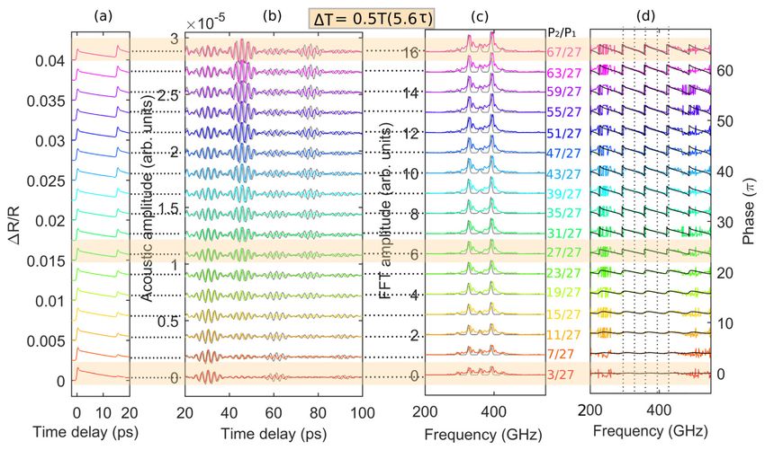
Vol. 27, No. 13 | 24 Jun 2019 | OPTICS EXPRESS 18707

magnetic field stimulation in ferrite [14], integrated phononic circuitry [15], and acoustic
nanocavities [16,17]. The straightforward way to manipulating CAPs on a picosecond time
scale is to do so in tailored nanostructures and materials, since the properties of laser-induced
coherent picosecond acoustic phonons are strongly dependent on the nature of the constituent
layers, their thicknesses, and periods of layered structures or thin-films [18]. For example,
frequencies and frequency differences within the observed triplets of zone-folded acoustic
phonon modes were studied in GaAs/AlAs superlattices with different combinations of GaAs
and AlAs monolayers [19]. In addition to the frequency, the acoustic amplitude and phase can
also be modulated by the choice of layer thickness. In thin GaP films grown on a silicon
substrate, both the amplitude and the phase of acoustic phonon time traces have been shown
to vary with the GaP layer thickness in a wide range [20]. Material tailoring offers another
possibility to adjust the acoustic phonon amplitude and frequency. For instance, InxGa1-xN
epilayers with various Indium composition x, led to a change of the amplitude of the acoustic
oscillations proportional to the Indium composition [21]. Apart from the direct influence of
sample structures and materials, the extrinsic factors such as external electric fields,
temperature, pressure, and magnetic fields are also crucial to the CAP processes. Because the
electronic properties of specific samples such as the energy band structure and dielectric
constants can be tailored by temperature and pressure, additionally, the optical field inside
materials can be modified by external electric and magnetic fields, leading to variations in
light absorption and light scattering [22]. In turn, the photo-excited CAP processes are
perturbed via electron-phonon, phonon-phonon and photon-phonon interactions. Hence, those
extrinsic factors can also be applicable to tune acoustic phonons. For example, control of the
CAPs amplitude was demonstrated by introducing external biases in a piezoelectric
InGaN/GaN multiple quantum wells (MQWs) structure in the range from +2 V to −9 V [23].
The CAPs damping and amplitude were modulated by the temperature variation from 4.5 K
to 300 K in a quantum cascade laser structure [24].
    Even though the above approaches for CAP manipulation have displayed their feasibilities
and versatilities, many questions remain open. While these questions could be answered by
investigating a large number of different sample structures and using a large set of parameters
for the variation of extrinsic factors, we decide to invest the control over CAP dynamics
optically. Since CAPs are excited by lasers in ultrafast time-resolved spectroscopy, excited
CAP features are considerably dependent on optical pulse properties. For example, the
adjustment of pump light wavelength can result in the phonon pulse shape variation due to the
altering of optical absorption spectra in a triple-quantum-well structure [25]. The optical
pump power influence on the CAPs amplitude in a ZnO/ZnMgO MQWs structure, induced by
the variation of photo-excited carriers and the screening effect, was also examined [26]. On
the basis of the ultrafast optical single-pulse coherent control of CAP via optical pulse
parameter modifications, the multiple-pulse optical manipulation of CAPs has arisen
increasing attention and attained noticeable progress, which enables selective excitation in
superlattices [27,28], MQW structures [29,30], nanoparticles [31], plasmonic nanostructures
[32] and aluminum gratings [33], frequency tuneabilities in single quantum well structures
[34] and thin films [35], and phase shifts in a MQW structure [36]. The multiple pulses are
normally split from the pump source and adjustable time intervals between them are applied
by introducing variable delay lines, hence constructive or destructive acoustic phonon
excitations take place in the structure, depending on the time delay between them. More
complex phonon control can be realized by simultaneous multi-parameter modulation of
multiple optical pulses, which can take advantage of the ultrafast optical pulse shaping
technique that enables user-defined almost arbitrary optical waveforms by a pulse shaper such
as a spatial light modulator exerted on spectrally decomposed laser pulses [37]. Nonetheless,
mere double-pump-pulse schemes have already proven their viability to manipulate CAPs by
control of pump time intervals and pump intensities in semiconductor multilayer structures
[28–30,36]. We notice several characteristics of the most reported two-pump-pulse optical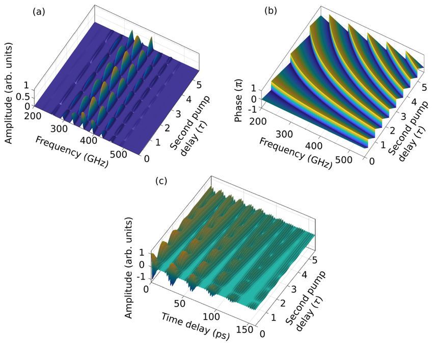
Vol. 27, No. 13 | 24 Jun 2019 | OPTICS EXPRESS 18708

control systems of coherent acoustic phonons. Firstly, Nd-doped solid lasers pumped
Ti:sapphire lasers are usually employed as pump and probe sources for pump-probe
spectroscopy, which leads to high-cost and bulky systems. Secondly, the employed
Ti:sapphire lasers mostly have a sub-GHz pulse repetition rate, which gives rise to a long time
window (>1ns) that is not necessary for some CAP processes on the time scale of a few
hundred ps. In addition, the systems with low repetition rate undergo a tradeoff between the
scan rate and the temporal resolution [38]. Thirdly, most of the CAPs manipulation
experiments are conducted in a conventional system where the time delay between the pump
and the probe pulse is realized by a mechanical delay line, which limits the scan speed (
Vol. 27, No. 13 | 24 Jun 2019 | OPTICS EXPRESS 18709

time window due to the relative timing jitter between the two lasers. The temporal resolution
is limited by the laser pulse duration (the pump and probe laser pulse durations are ~210 ps
and ~280 ps, respectively).The detection sensitivity is close to shot noise limit (noise floor
can be below ∆R/R = 10−6 in a few seconds). Differing from the original single-pump-pulse
set-up, the incident pump beam is split into two portions by a pellicle before collinearly
irradiating the sample in the normal direction. In the path of one of the split beams, a variable
mechanical delay stage is inserted in order to control the time interval between two pump
pulses, as illustrated in Figs. 1(b) and 1(c). For the adjustment of the pump intensity of the
delayed pump pulse, an adjustable neutral density filter (NDF) and a half wave plate (HWP)
are employed and inserted in the path of the delayed pulse. The NDF is capable of tuning the
pump power in the range of 0 – 37 mW and the HWP can extend the tunable range from 37
mW to 69 mW due to the pellicle transmission dependences on polarizations. The probe beam
is oblique with respect to the sample and its power is fixed at 4.5 mW. The reflectivity
variation of the sample after its excitation by the pump laser pulse is a function of the time
delay between the probe pulse and pump pulses, which is monitored by the reflected probe
light.

         Fig. 1. (a) The block diagram of ASOPS system. (b) The double-pump-pulse configuration in
         the measurement box. NDF: neutral density filter. NDF is used to adjust the delayed second
         pump power in the range of 0 – 37 mW. (c) The supplementary double-pulse-pump
         configuration in the measurement box. HWP: half wave plate. HWP is used to adjust the
         delayed second pump power in the range of 37 – 69 mW. (d) The sample structure. The
         multilayered sample is composed of GaAs layers (coral pink areas), In0.27Ga0.73As layers (QW,
         blue areas) and a DBR.

    The sample under investigation is a SESAM structure with multiple In0.27Ga0.73As
quantum wells (QWs) as saturable absorber ahead of a distributed Bragg reflector (DBR)
consisting of 23 pairs of GaAs/Al0.95Ga0.05As. The DBR reflects the incident light with a
reflectance of nearly 100%. Because the photon energy is above the bandgap of In0.27Ga0.73As
but below the bandgap of DBR constituent materials in the structure, light absorption occurs
only in the QWs. The structure of the sample is displayed in Fig. 1(d). The sample is grown
on a GaAs substrate along the [100] direction. Every three QWs and their barriers form a
triple-QW stack and in total three triple-QW stacks are formed. All QWs have the same
thickness of 7 nm and all barriers within a triple-QW stack also have the same thickness of 6
nm. The GaAs layer thickness between two adjacent triple-QW stacks is 112 nm while the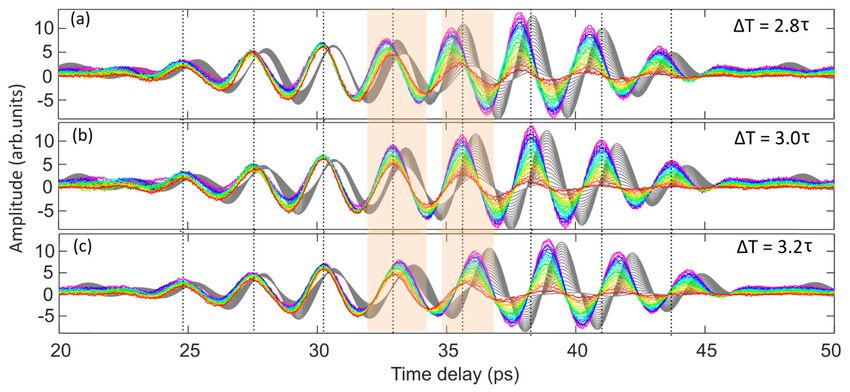
Vol. 27, No. 13 | 24 Jun 2019 | OPTICS EXPRESS 18710
thickness of the GaAs cap layer is 55 nm, which is approximately half of the stack-to-stack
distance. To clarify the notations, dQW denotes the distance between two adjacent QWs, which
also indicates the wavelength of laser-induced acoustic phonons in QWs; ds denotes the
thickness of the triple-QW stack; dss denotes the stack-to-stack distance. It will take excited
longitudinal acoustic phonons a time duration of T = dss/v ≈30.2 ps to travel through adjacent
triple-QW stacks (v = 4730 m/s in GaAs [41]). Because the periodic MQW structure is of
great interest for wave-packet-like coherent acoustic phonon manipulations, our following
acoustic discussions will focus on this region rather than the DBR. All experiments are
performed at room temperature.
3. Theoretical modelling
Once a pump photon is absorbed inside the QW region, electron-hole pairs are excited.
Hence, the electronic distribution in the QWs is disturbed and thus an initial stress is set up in
each QW via deformation potential [42]. The detailed stress distribution largely depends on
the space-time evolution of photo-excited charge carriers and physical properties of the
structure [2]. However, a detailed microscopic treatment of the electron dynamics is beyond
the scope of this work. As we will show in the following this does not hinder an already in
depth understanding of the undergoing acoustic dynamics.
Fig. 2. Illustration of the stress wave initiated in a triple-QW stack (solid curves) and detected
periodically (dotted lines) in an infinite MQW structure. The profile of a triple-QW stack is
assumed as (a) Gaussian shape and (b) rectangular shape.
Based on the structure of the triple-QW stack where the thickness of InGaAs is very close
to that of the GaAs barrier dInGaAs ≈dbarrier, and the wave-packet-like acoustic oscillations
displayed in our earlier measurements [39,40], it is reasonable to assume that the stress wave
generated in each triple-QW stack is a cosine wave enveloped by the profile of the stack. For
simplicity, we will initially assume that the stack generation profile exhibits a Gaussian
shape. The launched stress wave propagates simultaneously forward and backward along the
z-axis which is perpendicular to the QWs (see Fig. 2(a)). Due to the small acoustic impedance
difference between In0.27Ga0.73As and GaAs, the acoustic reflections on the interfaces are
neglected in our following analysis. In addition, considering that the counter-propagating
stress waves have the equivalent impact on the final acoustic response, we will not specify the
stress wave propagation direction in our mathematical analysis. To begin with, we consider
the excitation by a single pump pulse in one triple-QW stack. The generated stress wave can
be expressed as a function of space z and time t
( z − vt )2 2π
f g ( z , t ) = a exp − cos ( z − vt ) , (1)
2σ 2
d QW
where a is a constant, indicating the stress wave amplitude, v denotes the longitudinal acoustic
velocity in the sample, dQW denotes the QW-to-QW distance. Because the sound velocities are
nearly equal vInGaAs ≈vGaAs [40], for simplicity in the modelling, we assume that acoustic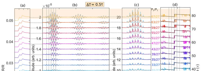
Vol. 27, No. 13 | 24 Jun 2019 | OPTICS EXPRESS 18711
waves are travelling everywhere in the MQW structure at the speed of v = vGaAs. The standard
deviation σ in the Gaussian formula can be given as
ds
σ= , (2)
2 2 ln 2
where ds denotes the triple-QW stack thickness, defined as the full width at half maximum
(FWHM) of the Gaussian profile. When the stress waves travel along the z-axis in the sample,
the vibration perturbs the refractive index and thus the probe light will monitor its
modifications via photoelastic effect. In our ASOPS system, the probe Yb:KYW laser is
nearly identical to the pump laser in terms of the central wavelength, the pulse-width, and the
pulse repetition rate. Thereby, the stress detection sensitivity function is assumed to share the
same form with the stress generation function, written as a function of z
z2 2π
f d ( z ) = b exp − 2 cos z , (3)
2σ d QW
where b is a constant. Equation (3) only represents the detection sensitivity function of a
single triple-QW stack, for the compact presentation of the following integration calculation.
The final acoustic waves detected by all triple-QW stacks will be discussed later where
necessary. The induced temporal signal response can be regarded as the convolution of the
stress wave generation function and the detection sensitivity function
∞
s1 ( t ) = f d ( z ) ∗ f g ( z ) = f d ( z ) f g ( z , t ) dz . (4)
−∞
If Eqs. (1) and (3) are substituted into Eq. (4), the following expression is obtained:
z2 ( z − vt ) 2π
2
∞ 2π
s1 ( t ) = ab exp − 2 − cos ( z − vt ) cos z dz
2σ 2σ 2
d QW d QW
−∞
1 vt 2 2π
= ab exp − c1 + c 2 cos vt (5)
2 2σ d QW
vt 2 2π
≅ c3 exp − cos vt .
2σ d QW
In Eq. (5), c1, c2 and c3 are constants. The integral calculation indicates c1 ≅ 0 c2, therefore,
c1 can be ignored. The final expression in Eq. (5) is associated with the high-frequency
oscillation which shows a wave-packet-like behavior. Then we will perform Fourier
transform to s1(t) as follows
∞
S1 ( f ) = s1 ( t ) exp ( −i 2πft ) dt
−∞
f − f 2 f + f 2 (6)
= c4 exp − 0
+ exp −
0
,
v / ( 2πσ )
v / ( 2πσ )
where c4 is a constant and f0 = v/dQW, indicating the frequency of acoustic oscillation in the
triple-QW stack. The result in Eq. (6) implies that the envelope of the acoustic spectrum also
has a Gaussian shape with the central frequency f0 and the bandwidth ∆BFWHM = (ln
2)1/2v/(πσ). It is noteworthy that the spectrum is real, which means the spectral phase equals
zero in the frame of our modelling. So far only a single triple-QW stack is taken into account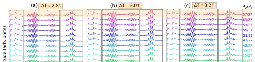
Vol. 27, No. 13 | 24 Jun 2019 | OPTICS EXPRESS 18712
in the acoustic phonon generation and detection process. However, the triple-QW stack
spatially repeats with the equal distance dss in the structure, which means the stress waves
initiated in the triple-QW stack subsequently propagate in both forward and backward
directions, and are detected in the equally distributed triple-QW stacks at times t = ndss/v =
nT, where n = 1, 2, 3, … (see Fig. 2(a)). As the illustration indicates, the MQW structure is
assumed to be infinite along the z- axis, which permits us not to take into consideration the
reflection on the air/sample boundary and simplifies the calculation. Because the cap layer
thickness approximately equals half of the thickness of the GaAs layer sandwiched by two
neighboring triple-QW stacks, the assumption of simply repeated triple-QW stacks without
the air/sample interface reflection makes sense in our calculation. In addition, it is worthwhile
mentioning that the stress waves are excited in all triple-QW stacks at the same time although
only the excitation by a single triple-QW stack is illustrated and analyzed above. The
combined excitation by all the triple-QW stacks only leads to larger acoustic intensity
compared to a single triple-QW stack excitation. Finally, concerning the damping of the
wave-packet sequence potentially induced by defect scattering, the stress wave sign change
by the reflection on the air/GaAs interface, and the limited number of triple-QW stacks in the
physical structure, we assume that the time-domain acoustic signal is enveloped by a
Gaussian shape h(t). Hence, taking into account the temporally periodically repeated wave-
packets, the overall damping and the amplitude magnification, the final acoustic response can
be expressed as
nd
s1_total ( t ) = c5 n =−∞ s1 t − ss h (t )
∞
v
1 2 2 ln 2 2 (7)
nd
= c5 n =−∞ s1 t − ss
∞
exp − 2 Δt t ,
2
v
where c5 is a constant and ∆t represents the pulsewidth (FWHM) of the superimposed
Gaussian envelope. The Fourier transform is then applied to Eq. (7) as follows
∞ nd
S1_total ( f ) = c5 n =−∞ s1 t − ss h ( t ) exp ( −i 2πft ) dt
∞
−∞
v (8)
= c6 m =−∞ S1 ( f ) H ( f − mΔf ),
∞
where c6 is a constant, m is an integer, and ∆f denotes the spectral comb spacing with the
relation ∆f = v/dss. H(f) represents the Fourier transform of h(t). We then substitute Eq. (6)
into Eq. (8) and apply a Fourier transformation to h(t), so the final acoustic spectrum in the
MQW structure analyzed in the single-pump-pulse configuration can be presented as
S1_total ( f ) =
f − f 2 f + f 2 (9)
2
f − mΔf
c7 m =−∞ exp −
∞
+ exp − exp − ,
0 0
v / ( 2πσ ) v / ( 2πσ ) 2 2 ln 2 / ( πΔt )
where c7 is a constant. Equation (9) reveals four features of the spectral response. Firstly, the
amplitude spectrum is composed of comb-like components spaced by ∆f which is determined
by the triple-QW stack-to-stack spacing and the longitudinal acoustic velocity. The spectrum
is real. Secondly, the comb spectrum is centered at f0, determined by QW-to-QW spacing
within a triple-QW stack and the longitudinal acoustic velocity. Thirdly, the comb
components amplitude is enveloped by a Gaussian shape associated with the acoustic
generation and detection profile in the triple-QW stack. Equation (9) together with Eq. (2),
indicates that the bandwidth of the comb spectrum is inversely proportional to the thickness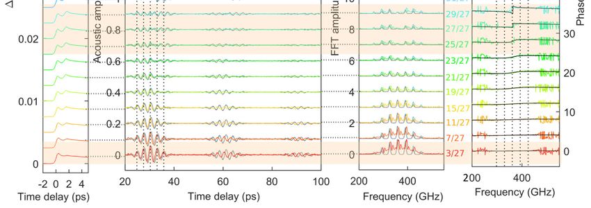
Vol. 27, No. 13 | 24 Jun 2019 | OPTICS EXPRESS 18713
of the triple-QW stack. Lastly, the comb linewidth is related to the acoustic temporal damping
window duration.
In the same way, if a rectangular generation and detection profile with width equal to ds in
the triple-QW stack is assumed (see Fig. 2(b)), the following spectrum can be derived
S1R_total ( f ) =
(10)
2
1 2 f − f 0 1 2 f + f 0 f − mΔf
c8 m =−∞
∞
sin + sin exp − ,
( f − f )2 v / (πd s ) ( f + f 0 ) 2 2 ln 2 / ( πΔt )
2
0 v / (πd s )
where c8 is a constant. Unlike the spectrum under the assumption of a Gaussian profile, the
spectrum derived from a rectangular generation and detection profile, shows that the acoustic
comb components are modulated by the square of a sampling function and thus show a clear
distinction regarding spectral bandwidth and comb component amplitudes compared to the
Gaussian assumption.
We will now move on to the double-pump-pulse situation, performing the analysis in the
spectral domain. Two key variables are introduced to demonstrate the acoustic manipulation
by a double-pump-pulse scheme, namely, the time delay ∆T between the first and the second
pump pulse and the pump power ratio q = P2/P1 where P1 and P2 are the pump power for the
first and the second beam, respectively. For a given pump laser, the pump pulse intensity is
proportional to the pump power and slight beam spot size variations induced by divergence
when ∆T is adjusted are ignored, so the pump power ratio is considered the same as pump
pulse intensity ratio in our analysis. We start with a brief discussion of the pump power effect.
As a saturable absorber incorporated in the SESAM structure, the In0.27Ga0.73As QW layers
lead to a nonlinear reflectivity curve dependent on the incident pulse fluence, because the
saturation absorption takes place when the initial states for the pump light transitions are
bleached while the final states are still occupied at high optical pump fluence [43,44].
Therefore, the amplitude of photo-excited acoustic phonons potentially does not follow a
linear relation with the incident pump power as well. However, initially we will assume that
the phonon amplitude is proportional to the incident pump power for simplicity as follows
A2 P2
= = q, (11)
A1 P1
where A2 and A1 denote the amplitude of CAPs excited by the first pump pulse and by the
second pump pulse, respectively. In Section 4, we will improve our model by nonlinear
corrections. Secondly, in addition to the varied pump power, the excitation by the sequential
pump light with changing time intervals ∆T also gives rise to subtle modifications of carrier
dynamics in the QWs [45], which is interesting for preventing multi-pulsing phenomena or
for the development of high repetition rate lasers by observing the optical absorption.
However, we will not further explore its effect on acoustic phonons, but simply neglect the
potential consequence in the modelling. In the time domain, the double-pump-pulse induced
acoustic response can be written as
s2_total ( t ) = s1_total ( t ) + qs1_total ( t − ΔT ) . (12)
The corresponding acoustic response in the spectral domain is thus derived as follows
S 2_total ( f ) = S1_total ( f ) + qS1_total ( f ) exp ( −i 2πf ΔT )
(13)
= S 2_total ( f ) exp iθ ( f ) .
The amplitude spectrum |S2_total(f)| and phase spectrum θ(f) can be expressed as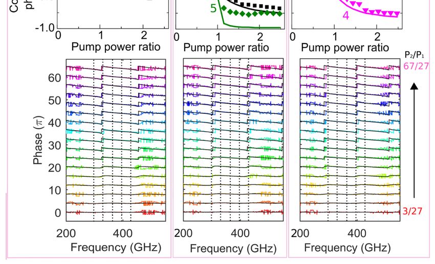
Vol. 27, No. 13 | 24 Jun 2019 | OPTICS EXPRESS 18714
S 2_total ( f ) = S1_ total ( f ) (1 − q ) + 4q cos 2 ( πf ΔT )
2
(14)
and
−q sin ( 2πf ΔT )
θ ( f ) = tan −1 , (15)
1 + q cos ( 2πf ΔT )
respectively. Equations (14) and (15) indicate that both the acoustic spectral amplitude and
phase are modulated simultaneously by the pump intensity ratio q and the time delay between
two successive pump pulses ∆T. Several interesting facts are unveiled as follows. Firstly,
when q is fixed, the amplitude variation of the spectral comb components is periodic with
varying ∆T. Moreover, the frequency of the periodic variation is equivalent to the spectral
frequency f. Secondly, if the comb frequency f = m∆f (m = 1, 2, 3, …) is substituted into Eq.
(14), the local minimum of the spectral amplitude variation with q can be found at q = 1 for
the mth comb component where m satisfies m = (2n + 1)/(2∆f∆T) (n = 0, 1, 2, …) and is an
integer number for the particular values of ∆T. Thirdly, the spectral phase also shows a
periodic variation dependent on ∆T, when q is fixed.
In the next section, the experimental CAP results attained in the double-pump-pulse
ASOPS system will be given, meanwhile, the modelling will be visualized for comparison.
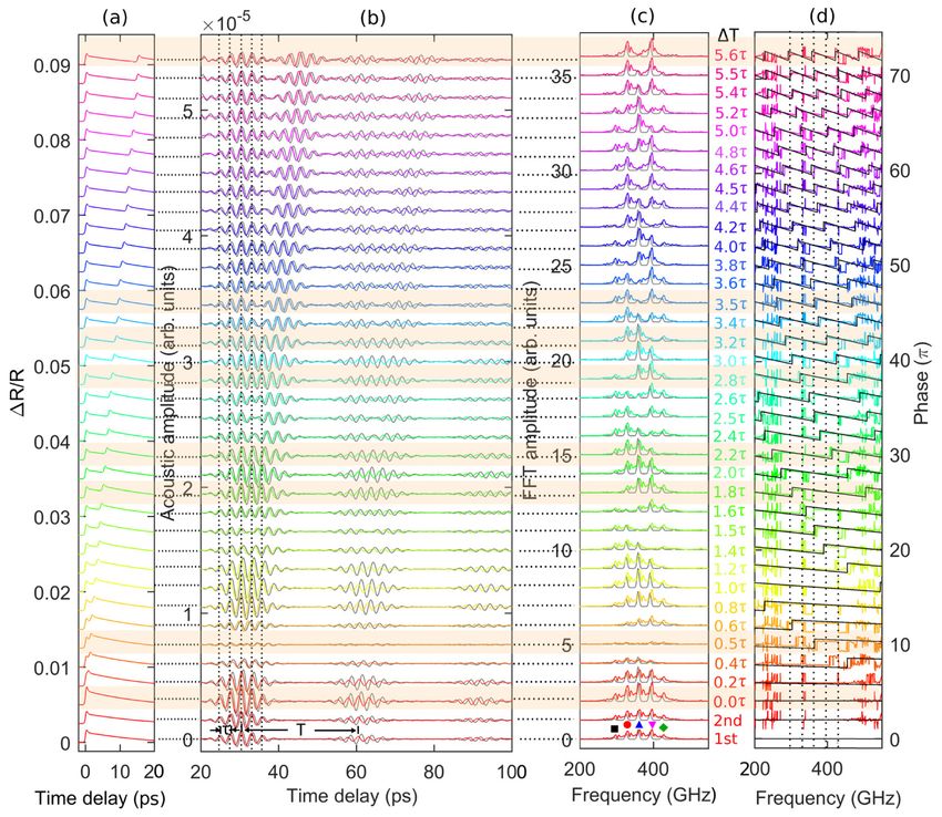
Fig. 3. (a) Original time traces, (b) coherent acoustic phonons, (c) acoustic amplitude
spectrums, and (d) acoustic phase spectrums when the second pump time delay ∆T varies in
the range of 0 – 5.6τ (0.5T). The first pump power P1 equals the second pump power P2 of 27
mW. Curves with ∆T-dependent color represent experimental results and gray curves represent
modelling results given Gaussian generation and detection functions in individual triple-QW
stack. Vertical dot black lines in (d) indicate the positions of five comb frequencies. Data are
shifted vertically for clarity in steps of 2.5 × 10⁻³ in (a), 1.5 × 10⁻⁶ in (b), 1 in (c) and 2π in (d).
Vol. 27, No. 13 | 24 Jun 2019 | OPTICS EXPRESS 18715

4. Experimental results and modelling visualization
For clarification, experimental acoustic waves presented in this section are obtained by
numerically removing the electronic and thermal exponential decaying background from the
original reflectivity change (∆R/R) traces via a smoothing average method. Thus the small
acoustic signal becomes visible and coherent control over acoustic waves can be observed.
4.1 Tunable pump delay, fixed pump power
Previously we have described and discussed CAPs excited in the same MQW structure by a
single-pump-pulse ASOPS system based on two Yb:KYW lasers, where an acoustic wave-
packet temporal sequence was produced, due to spatially periodically distributed triple-QW
stacks [39,40]. Aiming to optically coherently controlling the CAPs in this structure, a second
pump pulse with tunable time delay ∆T and tunable pump power P2 is introduced in the
experimental set-up.
    Initially, the optical power of the second pump light is kept equal to that of the first one at
27 mW, meanwhile, the time delay ∆T between two pump pulses is adjustable in the range
from 0 to 0.5T (5.6τ) which equals 15.12 ps in our case by moving a variable delay stage,
where T and τ denote the period of the acoustic wave-packet sequence and the period of
oscillations within the individual acoustic wave-packet, respectively. Consequently, a series
of distinct coherent acoustic phonons is obtained by tuning only the time delay ∆T and
displayed by curves with ∆T-dependent color in Figs. 3(a)-3(d) in forms of the original pump-
probe time traces, the subtracted temporal acoustic phonons, and the acoustic spectral
amplitudes and spectral phases. For comparison, the single-pump-pulse measurements with
only the first pump beam and only the second pump beam incident are performed, as depicted
in the first and second curves at the bottom of Figs. 3(a)-3(d). The five equally spaced
pronounced frequency comb components at f1 = 297.8 GHz, f2 = 330.5 GHz, f3 = 363.2 GHz,
f4 = 396.4 GHz and f5 = 428.2 GHz are defined as comb1, comb2, comb3, comb4 and comb5
(from left to right, marked by a black, red, blue, magenta and green symbol in Fig. 3(c)),
respectively, which will be discussed in terms of acoustic amplitude and phase variations
throughout Section 4. Compared to the single-pump-pulse acoustic phonons, the double-
pump-pulse acoustic phonons amplitudes are evidently enhanced at ∆T = 0.0τ and suppressed
at ∆T = 0.5τ for all five comb components. Subsequently, they are also enhanced at ∆T = 1.0τ,
2.0τ, 3.0τ, 4.0τ while almost cancelled out at ∆T = 1.5τ, 2.5τ, 3.5τ, 4.5τ in the temporally
overlapping region of the wave-packets excited by the first pump pulse and those excited by
the second pump pulse. Depending on the time delay ∆T, it is possible to almost extinguish
certain frequency comb components. For instance, at ∆T = 1.8τ, 2.2τ, 2.8τ, 3.2τ, and 3.5τ,
comb1, comb5, comb2, comb4, and comb3 are greatly suppressed, respectively. In other
words, all five comb components can be individually controlled to be present or absent in the
spectrum by selecting a specific time delay ∆T, which could be very useful for filtering out
the unwanted acoustic spectral components if required in certain applications. At the specific
time delay ∆T = 5.6τ ≅ 0.5T, it is noticeable that odd spectral components are suppressed,
leading to a doubled frequency comb spacing and a reduced temporal wave-packet period to
T/2.
    Not only the spectral amplitude but also the spectral phase is dependent on the second
pump time delay ∆T, as shown in Fig. 3(d). In order to eliminate the initial phase caused by
the temporal range selection (20 – 250 ps) for Fourier transform and other potential
perturbations in the experiment, the spectral phase resulting from the double-pump-pulse set-
up is displayed as a result of relative spectral phase with respect to that obtained in the single-
pump-pulse set-up. The simultaneous spectral amplitude and phase modulation by tuning ∆T,
enables a variety of acoustic wave-packet sequences, where the shape, the width and the
amplitude of the individual wave-packet can be modified flexibly, leading to a quasi-arbitrary
acoustic wave-packet shaping, as depicted in Fig. 3(b). The maxima corresponding to single-
Vol. 27, No. 13 | 24 Jun 2019 | OPTICS EXPRESS 18716
period oscillations composing an individual wave-packet experience phase shifts
approximately from - π to π, depending on ∆T. For example, the oscillation at 35.6 ps is out of
phase at ∆T = 1.4τ compared to the single-pump-pulse data (the fifth peak in the first wave-
packet in Fig. 3(b)). Based on the theoretical modelling in the last section, the acoustic
calculation under the assumption of a Gaussian triple-QW generation and detection profile is
applied in the condition of tunable ∆T and fixed q = 1, as depicted by solid gray (black)
curves in Figs. 3(b)-3(d). The comparison of experimental curves and calculation curves
indicates that our modelling achieves good agreement with the experimental results in the
tunable ∆T range in both the temporal and spectral domain.
Fig. 4. (a) The amplitude of five main frequency comb components at 297.8 GHz, 330.5 GHz,
363.2 GHz), 396.4 GHz and 428.2 GHz as a function of the second pump time-delay from 0 to
5.6τ. Solid lines denote the absolute cosine fit for experimental results by y(t) = |cos(πft)|. (b)
The relation between the modulation frequencies from (a) and the corresponding comb
component frequencies.
Fig. 5. (a) The phase shift of five main frequency comb components at 297.8 GHz, 330.5 GHz,
363.2 GHz, 396.4 GHz and 428.2 GHz as a function of the second pump delay from 0 to 5.6τ.
(b) The relation between the phase modulation frequencies from (a) and the corresponding
comb component frequencies.
The slight discrepancy between the experiment and the modelling (~0.3 ps for peaks in the
first wave-packet and ~5 GHz for spectral comb components) can be attributed to the
uncertainty of determination of the acoustic velocity in the sample and the nominal QW-to-
QW width and stack-to-stack width. The high baseline shown in experimental amplitude
spectrum is mainly caused by numerical Fourier transform window. Because the strongestVol. 27, No. 13 | 24 Jun 2019 | OPTICS EXPRESS 18717
wave-packets are at the beginning of the time delay and the wave-packet sequence has a fast
decay, a sharp-edged window is used to preserve the main signal so that the spectral
information will be more reliable although a high baseline can be caused. The baseline can be
lower if a Gaussian-like window is chosen, however, most visible wave-packets would be
suppressed in this case, leading to a weak noisy spectrum. Potentially, the high baseline could
be partly caused by the sample fabrication issues such as inhomogeneities and defects. The
unexpected spectral phase jump and the irregular phase appearing in the experiment could be
caused by the experimental noise (the acoustic signal is small beyond the range
approximately from 290 GHz to 430 GHz, so the phase in those small-signal regimes is easy
to be disturbed by the noise) and numerical operations. The lateral phase deviation between
experiments and calculations probably stems from the imperfect accuracy to determine ∆T by
adjusting the variable translation stage.
In order to find out how the spectral comb amplitude and phase are quantitatively
dependent on the second pump delay ∆T, the amplitude and phase of the five main spectral
comb components are extracted from Figs. 3(c) and 3(d). In Fig. 4(a), ∆T-dependent
amplitudes of comb1, comb2, comb3, comb4 and comb5, display an apparent cosine-wave-
like variation, with a peak amplitude ratio of 0.40:0.83:0.94:1.00:0.43 and a decreasing period
of τ1 = 1.23τ, τ2 = 1.11τ, τ3 = 1.01τ, τ4 = 0.93τ and τ5 = 0.86τ, respectively. On the one hand,
the periodic evolution of individual comb components at different speed permits various
comb amplitude profiles and the periodic removal of a certain component. On the other hand,
a complete extinction of all comb components at the same ∆T is not possible. At ∆T = 0.5τ,
only comb3 is almost completely suppressed and other four comb components remain finite
although with a small amplitude. The cosine-wave-like behavior can be explained very well
by Eq. (14) in Section 3, where the spectral amplitude is modulated by a factor |cos(πf∆T)|
when q = 1, indicating that the amplitude evolution with the time delay ∆T is a periodic
variation following modulus of cosine with a frequency of f. Importantly, the factor reveals
that the modulation frequency of this variation for a comb component is exactly equivalent to
the frequency of the comb component itself. We illustrate the relation of the frequency of the
five amplitude modulations from Fig. 4(a) and the corresponding frequency of comb
components in Fig. 4(b) where the linear fit slope is very close to 1, which clearly
corroborates our above interpretations. Like the spectral amplitude evolution, the spectral
phase also exhibits a periodic variation, depending on the second pump delay ∆T (see Fig.
5(a)). However, the phase shift curve for each comb component is sawtooth-wave-like in the
phase range approximately from –π/2 to π/2. The linear fit with a slope of ≅1 in Fig. 5(b) also
indicates that the frequency of phase modulation equals the frequency of the corresponding
comb component. The explanation of the periodic behavior can be found in Eq. (15), where
the inverse tangent contains a numerator of -sin(2πf∆T) and a denominator of 1 + cos(2πf∆T)
(when q = 1) which are both periodic waves with a frequency of f as a function of ∆T, leading
to the periodic phase shift evolution with the period of 1/f for the comb component with a
frequency of f. At last, by illustrating simultaneous spectral amplitude modulation (see Fig.
6(a)) and phase modulation (see Fig. 6(b)) in the range of the second pump delay ∆T = 0 –
5.6τ with tiny ∆T steps, we emphasize several points in the following.
Firstly, both the spectral amplitude and the spectral phase dependences on ∆T change
faster when the spectral frequency is higher, leading to numerous amplitude and phase
combinations for the main five comb components.
Secondly, our result offers another approach to measure the frequency of acoustic
phonons, considering that the frequency of the periodic spectral amplitude and phase
dependences on ∆T for a comb component equals the frequency of the comb component
itself.
Thirdly, the amplitude of each comb component is restricted in the range from 0 to
2|S1_total(f)|, where|S1_total(f)| represents the spectral component amplitude of single-pump-pulse
acoustic phonons, while the spectral phase is restricted in the range from –π/2 to π/2. The π/2Vol. 27, No. 13 | 24 Jun 2019 | OPTICS EXPRESS 18718
(or -π/2) phase restriction is attributed to the fact that the denominator 1 + cos(2πf∆T)
periodically equals zero when ∆T satisfies ∆T = (2n + 1)/ (2f) (n is an integer).
Fourthly, the produced temporal acoustic wave-packet sequences as a consequence of
simultaneous spectral amplitude and phase modulation demonstrate various interference
patterns of acoustic phonons, which shape the discrete individual wave-packets, depending on
the second pump delay ∆T, as shown in Fig. 6(c).
To sum up, by only adjusting the time delay ∆T between two successive optical pump
pulses in the range of 0 – 5.6τ, we have experimentally shown that acoustic phonons are
coherently controlled by periodic comb amplitude and comb phase modulations, leading to an
almost complete suppression of certain comb components at certain time delays ∆T, which is
well supported by our theoretical modelling.
In addition to the second pump delay ∆T, the pump power ratio q is also adjustable in our
system. Hence, in the following we will explore whether it is feasible to modulate acoustic
phonons by tuning q at a fixed ∆T. For example, we will examine if the almost extinct comb
component can be revived by changing q and if the spectral amplitude and phase range can be
extended compared to the case where q = 1.
4.2 Tunable pump power, fixed pump delay
4.2.1 Pump delay ∆T = 0.5τ
As the first example, we introduce the adjustment of the pump ratio q at the fixed ∆T = 0.5τ
which gives rise to immense acoustic suppression at q = 1. In the experiment, the power of
the first pump light is fixed at 27 mW while that of the second pump light is tunable from 3
mW to 67 mW. The experimental and theoretical results are present in Figs. 7(a)-7(d). The
experimental results (see curves with q-dependent color) will be discussed first.
Fig. 6. The acoustic calculation based on the assumption of a Gaussian generation and
detection profile of the triple-QW stack. The pump power ratio is fixed at q = 1 and the second
pump pulse delay ∆T is adjustable in the range of 0 – 5.6τ . (a) The comb frequency
component amplitude dependences on the second pump pulse delay. (b) The comb frequency
component phase dependences on the second pump pulse delay. (c) The corresponding
variation of coherent acoustic phonons as a function of the second pump pulse delay.Vol. 27, No. 13 | 24 Jun 2019 | OPTICS EXPRESS 18719
Although the acoustics are greatly suppressed at q = 27/27, the spectral comb components
are not completely wiped out by adjusting the second pump delay ∆T. As indicated in Fig.
7(c), the complete removal can be realized by fine tuning q in the vicinity of q = 1 neither,
which can be interpreted with the assistance of Eq. (14) where the amplitude modulation
factor [(1 - q)2 + 4qcos2(πf∆T)]1/2 exhibits zero value at ∆T = 0.5τ only in the condition of q =
1 and f = (2m + 1)/τ (m is an integer). Due to the relation 1/τ ≈f3, the factor has a dip only at
comb3 while the other four comb components can be suppressed to some extent because they
are in the vicinity of the dip. On the contrary, tuning q enables the suppressed comb
components to grow gradually back when q > 1 and q < 1 (see Fig. 7(c)). Take comb3 for
instance, the amplitude ratio at q = 3/27, 27/27, 67/27 is 0.92:0.08:0.88 obtained from the
experimental results, which proves that acoustic phonons can also be modulated by tuning the
pump power ratio q. It is worth noticing that the comb amplitude has a minimum at around q
= 27/27 and displays a saturation feature at high q (see Fig. 7(c)), and the comb phase also
shows a saturation tendency when q > 27/27 (see Fig. 7(d)). The phase variation with
frequency is slow, which is caused by the large period 2/τ ≅ 2f3 at ∆T = 0.5τ based on Eq.
(15).
Fig. 7. Comparison of experimental, Gaussian and rectangular modelling results. The pump
power ratio q = P2/P1 varies from 3/27 to 67/27 and the second pump delay is fixed at 0.5τ.
The first pump power is fixed at 27 mW in experiments. (a) Original time traces. (b) Coherent
acoustic phonons. (c) Acoustic amplitude spectrums. (d) Acoustic phase spectrums. Curves
with q-dependent color represent experimental results. Gray curves in (b) and (c) represent
Gaussian modelling results. Sky blue curves in (b) and (c) represent rectangular modelling
results. Black solid curves in (d) represent modelling results. Vertical dot black lines in (d)
indicate the position of five comb components. Data are shifted vertically for clarity in steps of
2.5 × 10⁻³ in (a), 1.0 × 10⁻⁶ in (b), 1 in (c) and 4π in (d).
In the temporal domain, acoustic phonons also experience interesting alterations (see Fig.
7(b)). Firstly, the leading part or the trailing part of the individual wave-packet can be
selectively suppressed. For example, at around q = 21/27, the trailing half part is suppressed,
while at around q = 35/27, the leading half part is suppressed. Secondly, some single-periodVol. 27, No. 13 | 24 Jun 2019 | OPTICS EXPRESS 18720
oscillations composing the wave-packet undergo a phase shift of π when q is approximately
larger than 27/27 with respect to those at q = 3/27. At q = 67/27, all oscillations inside the
wave-packet exhibit a phase shift of π, which means the whole wave-packet sequence is
delayed by 0.5τ with respect to that at q = 3/27 (see the top curve and the bottom curve in Fig.
7(b)). For comparison, the acoustic calculations under the assumption of a Gaussian and
rectangular triple-QW profile are both given in the case of tunable q and fixed ∆T = 0.5τ,
which are illustrated in Figs. 7(b) and 7(c) by gray curves and sky-blue curves, respectively.
The phase calculation is illustrated by black curves in Fig. 7(d). As can be seen, the temporal
acoustic waves and the spectral amplitude and phase in general fit well with the experimental
results.
However, at high q, the calculation of the temporal acoustic amplitude and the spectral
amplitude obviously surpasses the corresponding experimental amplitude, because a linear
relation between pump power and acoustic amplitude is assumed in the calculation. Hence, in
the following a nonlinear factor k0 for spectral comb components, which should make pump-
power-acoustic-amplitude relation more realistic, will be introduced to improve our
modelling.
Moreover, the assumption of a Gaussian triple-QW detection and generation profile yields
a spectral bandwidth of 89.5 GHz, which is smaller than the experimental bandwidth of 109.6
GHz, leading to a comparatively smaller amplitude for comb1 and comb5 in the single-pump-
pulse experiment. The assumption of a rectangular one produces a spectral bandwidth of
127.6 GHz in the single-pump-pulse experiment, which is larger than the experimental
bandwidth, leading to additional dominant comb components. In addition, the overall
normalized component-to-component amplitude ratios show a discrepancy between the
calculation and the experiment (experiment: 0.4:0.86:0.96:1:0.5, Gaussian: 0.2:0.6:1:0.8:0.3,
rectangular: 0.4:0.8:1:0.9:0.5). Although a rectangular stress envelope is theoretically
expected, the finite detection and generation bandwidth can smear out the rectangular shape,
which potentially accounts for the deviation between the modelling and experiment results
regarding the spectral bandwidth and envelope. Because the double-pump-pulse modelling is
based on the single-pump-pulse analysis, the effect from the imperfect generation and
detection function is also impinged upon the double-pump-pulse acoustic phonons, as
illustrated in Figs. 7(b) and 7(c) at low q. Hence, we will also improve the spectral envelope
in the following by a heuristic-analytical method.
Fig. 8. (a) The experimental comb component amplitude dependences on the pump power
when only the second pump beam is incident on sample (filled symbols). The pump power
varies from 3 mW to 67 mW. The amplitude curves of five comb components are individually
fit linearly from 30 mW and exponentially from the beginning. Solid lines represent the linear
fit and dot lines represent the nonlinear fit. The nonlinear factor k0 (f, q) is the ratio between
the nonlinear fit and the linear fit. (b) Nonlinear factor curves k0(f, q) for five comb
components in the range of pump power ratio q = P2/P1 from 3/27 to 67/27.Vol. 27, No. 13 | 24 Jun 2019 | OPTICS EXPRESS 18721
In order to determine the value of the nonlinear factor k0, experiments with only the
second pump incident on the sample are performed in the range of the pump power from 3 to
67 mW with steps of 4 mW. As shown in Fig. 8(a) (filled symbols in five colors), the acoustic
spectral amplitude has a nonlinear relation with the incident pump power, which intrinsically
stems from the saturation absorption in the QWs of our sample and thus a nonlinear
reflectivity curve. An exponential fit is applied to the experimental data for five comb
components, starting from the lowest pump power (see dot lines in Fig. 8(a)), meanwhile, a
linear fit is applied to the experimental data starting from 30 mW (see solid lines in Fig. 8(a)).
The nonlinear factor k0 is a result of ratio between the exponential fit and the linear fit ranging
from 30 mW to 94 mW of the single pump power, as depicted in Fig. 8(b). Such a fitting
range is selected, because in the two-pulse-pump experiments the total incidence P1 + P2
ranges from (27 + 3) mW to (27 + 67) mW. The nonlinear factor k0 can be thus expressed as a
function of f and q
A1 ( f ) exp 27(1 + q ) / t1 ( f ) + A0 ( f )
k0 ( f , q ) = , (16)
a0 ( f ) + 27b0 ( f )(1 + q )
where A1(f), t1(f) and A0(f) are exponential fitting parameters at f = f1, f2, f3, f4, f5, while a0(f)
and b0(f) are linear fitting parameters at f = f1, f2, f3, f4, f5. The nonlinear factor is then
multiplied with the amplitude spectrum Eq. (14) to correct the exceeded acoustic amplitude at
high pump power induced by a linear relation assumption.
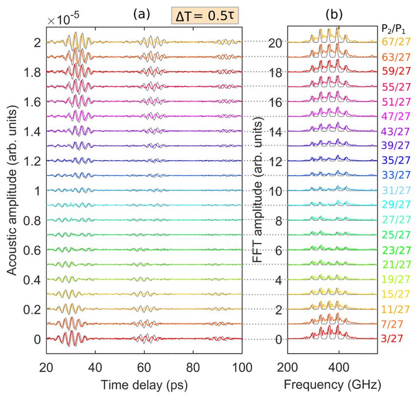
Fig. 9. Comparison of experimental and heuristic-analytical results after nonlinear corrections
in the range of q from 3/27 to 67/27 at ∆T = 0.5τ. (a) Time domain coherent acoustic phonons
and (b) corresponding acoustic spectrum series. Curves with q-dependent color represent
experimental results and gray lines represent the results after nonlinear corrections. Data are
shifted vertically for clarity in steps of 1.0 × 10⁻⁶ in (a) and 1 in (b).
The improvement of the generation and detection function is indirectly achieved by using
the experimental single-pump-pulse comb amplitude |S1_exp(f)| featured by the comb
components ratio 0.4:0.86:0.96:1:0.5 at 27 mW instead of using the derived |S1_total(f)| or
|S1R_total(f)| in Eq. (14). By combination of the nonlinear factor k0 corrections and heuristic-
analytical envelope corrections, the improved results are produced and displayed in Figs. 9(a)Vol. 27, No. 13 | 24 Jun 2019 | OPTICS EXPRESS 18722
and 9(b) (gray curves). In consequence, the acoustic phonons obtained from the improved
modelling fit well with the experimental acoustic phonons in the entire q range in both the
temporal and spectral domain. In Fig. 10(a), the amplitude of individual comb components
dependences on q after improvement by above two approaches (open symbols) in general
achieves a better agreement with experimental amplitude (filled symbols) than Gaussian-
based calculations after nonlinear factor corrections (dot lines) and rectangular-based
calculation after nonlinear factor corrections (cross signs). A few data points obtained from
the heuristic-analytical method show slightly larger deviations from experimental data at low
q than those obtained from the rectangular modelling do, however, this will not affect the
general improvements. The improved spectral amplitude is restricted by k0(f, q)|S1_exp(f)|[(1 -
q)2 + 4qcos2(πfτ/2)]1/2. Because the cosine term is close to zero at ∆T = 0.5τ for all five comb
components, the determination factor of the spectral amplitude can be regarded as k0(f,
q)|S1_exp(f)(1 - q)|, which is smaller than 2|S1_exp(f) | for all considered q.
In Fig. 10(b), the comb phase shift dependences on q demonstrate that, firstly, the phase
shift for all spectral comb components ranges approximately from 0 to π (or – π to 0);
secondly, the phase shift sign of comb1 and comb2 is opposite to that of comb4 and comb5;
thirdly, comb3 exhibits an abrupt phase change from ~0 to - π at around q = 1 (a few
experimental data points are discarded for comb3 due to their unexpected jump to the positive
side. This perhaps stems from the incorrect sign determination in the numerical phase
extraction. This also could be attributed to the inaccuracy of ∆T adjustment, which causes
phase shifts from the desired value and thus a sudden jump when the phase is close to the
wrapped phase “cliff” π (-π) (see Fig. 7(d)).); lastly, the phase saturation at high q can be
understood with the help of Eq. (15) where the right side term can be also written as tan−1{-
sin(2πf∆T)/[1/q + cos(2πf∆T)]}. Because 1/q approaches zero when q is large enough, the
term can be approximated as tan−1[–tan(π)] at ∆T = 0.5τ ≅ 0.5f3 for comb3, implying -π phase
at high q. Due to fi/f3 ≈1 (i = 1, 2, 4, 5), the phase for four other comb components is close to
π (or -π) at high q.
Fig. 10. (a) The comb component amplitude dependences on the pump power ratio q = P2/P1 at
∆T = 0.5τ. Filled symbols connected by solid lines represent experimental results. Open
symbols connected by solid lines represent heuristic-analytical results after nonlinear
corrections. Cross symbols connected by solid lines represent rectangular modelling results
after nonlinear corrections. Dot lines represent Gaussian modelling results after nonlinear
corrections. (b) The comb component phase dependences on the pump power ratio q = P2/P1 at
∆T = 0.5τ. Filled symbols represent experimental data and dot curves represent calculation
data. Gray straight lines are only for marking purpose.Vol. 27, No. 13 | 24 Jun 2019 | OPTICS EXPRESS 18723
4.2.2 Pump delay ∆T = 2.8τ, 3.0τ, 3.2τ
In addition to ∆T = 0.5τ, we also perform acoustic phonon manipulation by tuning the pump
power ratio at ∆T = 2.8τ, 3.0τ, 3.2τ for demonstration. When q = 1, the factor |cos(πf∆T)|
modulates the spectral amplitudes (see Fig. 4(a)). Then the following statements can be
concluded: at ∆T = 2.8τ, comb2 can be greatly suppressed because of the dip of comb2 at
2.5τ2 = 2.78τ; at ∆T = 3.0τ, comb1 and comb5 can be both greatly suppressed because of one
dip of comb1 at 2.5τ1 = 3.08τ and one dip of comb5 at 3.5τ5 = 3.01τ; at ∆T = 3.2τ, comb4 can
be greatly suppressed because of one dip of comb4 at 3.5τ4 = 3.26τ. τi (i = 1, 2, 3, 4, 5) is the
period of the cosine-wave-like amplitude dependences on ∆T for the comb component with
the frequency fi (i = 1, 2, 3, 4, 5), which were already defined in Section 4.1.
Fig. 11. The original time traces (left), coherent acoustic phonons (middle) and FFT spectrum
series (right) when the second and the first pump power ratio varies from 3/27 to 67/27. (a) ∆T
is fixed at 2.8τ. (b) ∆T is fixed at 3.0τ. (c) ∆T is fixed at 3.2τ. Curves with q-dependent color
represent experimental results and gray curves represent heuristic-analytical results after
nonlinear corrections. Data are shifted vertically for clarity.
Fig. 12. The first wave-packet of acoustic phonons when the pump power ratio varies from
3/27 to 67/27 (the data are the same as those in Figs. 11(a)-11(c), but smaller steps are used for
the vertical shift). The second pump delay is (a) ∆T = 2.8τ, (b) ∆T = 3.0τ, (c) ∆T = 3.2τ.
Vertical dot gray lines indicate the peak positions in the case of ∆T = 3.0τ at the pump ratio q =
3/27 (red). The colored curves from red to magenta represent experimental data from q = 3/27
to 67/27 (same as those curves in Figs. 11 (a)-11(c)). The gray curves represent heuristic-
analytical results after nonlinear corrections.Vol. 27, No. 13 | 24 Jun 2019 | OPTICS EXPRESS 18724
As illustrated in Figs. 11(a)-11(c), when ∆T keeps fixed, all the previously suppressed
comb components can be gradually revived by decreasing q or increasing q from q = 1,
meanwhile, other comb components in general experience a monotonically increasing
variation when q is increased from the lowest to the highest value. It is worth mentioning that
even at the lowest q = 3/27 (the second pump power is only 3 mW) the modulation made by
introducing the second pump is still totally visible. At the lowest q, the normalized
component-to-component amplitude ratios at ∆T = 2.8τ, 3.0τ, 3.2τ are 0.38:0.63:0.85:1:0.41,
0.34:0.75:1:0.95:0.35, 0.36:0.89:1:0.8:0.38, respectively. The capability to reveal an acoustic
manipulation at a very low pump power can be attributed to the high detection sensitivity of
our ASOPS system.
Fig. 13. Frequency comb component amplitude and phase dependences on the pump power
ratio q. (a) The second pump delay is fixed at 2.8τ. Top: comb component amplitude
dependences on q. Middle: comb component phase shift dependences on q. Filled symbols
denote experimental data, while solid lines denote heuristic-analytical results. The numbers 1,
2, 3, 4, 5 are used to address five comb components defined in Section 4.1. Bottom: spectral
phase in the q range from 3/27 to 67/27 in steps of 4/27. Curves with q-dependent color
represent experimental results and solid black curves represent heuristic-analytical results after
nonlinear corrections. Vertical dot black lines indicate the position of five comb components.
Phase spectrums are vertically shifted for clarity in steps of 4π. (b) The second pump delay is
fixed at 3.0τ. (c) The second pump delay is fixed at 3.2τ.
In the time domain, acoustic sequences composed of wave-packets with a variety of
profiles are produced. Because the wave-packet generated by the first pump and that
generated by the second pump light are nearly half-overlapped and have a constructive
interference at around ∆T = 3.0τ, the wave-packet remains a Gaussian-like shape whose width
is effectively prolonged, showing up to 8 single-period oscillations within each wave-packets.
Apart from the amplitude, the rise time of the wave-packet profile leading edge and the fall
time of the wave-packet trailing edge can be tuned by q. The comparison of the improvedVol. 27, No. 13 | 24 Jun 2019 | OPTICS EXPRESS 18725
modelling based results (gray curves in Figs. 11(a)-11(c)) with experimental results (curves
with q-dependent color in Figs. 11(a)-11(c)) demonstrates an excellent agreement in the
tunable q range at ∆T = 2.8τ, 3.0τ, 3.2τ in both the temporal and spectral domain. In order to
find out the subtle temporal pulse phase shift caused by tuning q, acoustic sequences are
shifted vertically in smaller steps (see Figs. 12(a)-12(c)). It is noticeable that the fourth
oscillation at 32.9 ps and the fifth oscillation at 35.65 ps have a positive phase shift
(maximum 0.15π (4th) and 0.26π (5th)) at ∆T = 2.8τ, a negative phase shift (maximum −0.11π
(4th) and −0.26π (5th)) at ∆T = 3.2τ, while a zero phase shift at ∆T = 3.0τ, by tuning q. At ∆T
= 2.8τ and 3.2τ, the maximum phase shift of single-period oscillations cannot reach π by
tuning q, while that can be achieved at ∆T = 0.5τ by tuning q.
The spectral amplitude and phase dependences on the pump power ratio q for the five
main spectral comb components at ∆T = 2.8τ, 3.0τ, 3.2τ are displayed in Figs. 13(a)-13(c). In
terms of the spectral amplitude dependences on q, the following points can be summarized.
Firstly, the amplitude dependences on q for some comb components are non-monotonic
while those for some other comb components monotonically increase with q. The selection of
comb component with a quadratic-function-like shape whose valley is at q = 1, depends on
the factor [(1 - q)2 + 4qcos2(πf∆T)]1/2 which indicates that the zero minimum only exists at q =
1 and f = (2m + 1)/(2∆T) (m is an integer). Therefore, at ∆T = 2.8τ ≅ 2.8/f3 and m = 2, the zero
minimum can be found approximately at f = 5f3/5.6 ≈f2 (see the top of Fig. 13(a)); at ∆T =
3.0τ ≅ 3.0/f3 and m = 2, 3, the zero minimum can be found approximately at f = 5f3/6 ≈f1 and f
= 7f3/6 ≈f5 (see the top of Fig. 13(b)); at ∆T = 3.2τ ≅ 3.2/f3 and m = 3, the zero minimum can
be found approximately at f = 7f3/6.4 ≈f4 (see the top of Fig. 13(c)). In order to explain the
local minimum point in the range of 0 ≤ q ≤ 1, we have to rely on the general local minimum
expression of q = -cos(2πf∆T), which indicates that the minimum exists in the range 0 ≤ q ≤ 1
when f∆T satisfies (4n + 1)/4 ≤ f∆T ≤ (4n + 3)/4 (n is an integer). For example, the comb1
amplitude at ∆T = 3.2τ has a minimum at q = 0.73 (see the top of Fig. 13(c)). When the
minimum is located in the range -1 ≤ q ≤ 0 under the condition (4n + 3)/4 ≤ f∆T ≤ (4n + 5)/4
or 0 ≤ f∆T ≤ 1/4 (n is an integer), we will observe a monotonically increasing amplitude
behavior of some spectral comb components. For example, the comb3 amplitude dependence
on q has a consistently rising tendency at ∆T = 2.8τ, due to the fact that the minimum of the
quadratic function locates at q = −0.31 (see the top of Fig. 13(a)).
Secondly, the maximum amplitude is restricted by the expression k0(f, q)|S1_exp(f)|[(1 - q)2
+ 4qcos2(πf∆T)]1/2 ≤ 2.6|S1_exp(f)|, which means that in Figs. 13(a)-13(c), unlike the case in
Section 4.1 and the case at ∆T = 0.5τ, the comb component amplitude can exceed 2|S1_exp(f)| at
high q and proper f∆T. For example, the maximum of comb3 amplitude at ∆T = 3.0τ is larger
than 2|S1_exp(f3)| ≈2A3(q = 3/27) (A3(q) denotes the amplitude of comb3, see the top of Fig.
13(b)).
In terms of the spectral phase dependences on q, the following points can be summarized.
Firstly, at ∆T = 2.8τ, 3.0τ, 3.2τ, the phase shift of all comb components shows a saturation
effect at high q, which can be explained in the similar way to the case at ∆T = 0.5τ.
Secondly, only a certain comb component can reach π or -π phase shift, which is
determined by whether the condition 2f∆T ≈2n + 1 (n is an integer) in tan−1[–tan(2πf∆T)] is
satisfied. For example, comb2 at ∆T = 2.8τ can reach π due to 2 × 2.8f2τ ≈5 (see the middle of
Fig. 13(a)); comb5 at ∆T = 3.0τ can reach approximately –π due to 2 × 3.0f5τ ≈7 (see the
middle of Fig. 13(b)); comb4 at ∆T = 3.2τ can reach up to approximately –π due to 2 × 3.2f4τ
≈7 (see the middle of Fig. 13(c)). However, the abrupt phase change around q = 1 takes place
only when the relation of f and ∆T satisfies 2f∆T = 2n + 1 (n is an integer) perfectly.
Thirdly, the modelling agrees also well with the experiment in the whole tunable q range
at ∆T = 2.8τ, 3.0τ, 3.2τ in terms of spectral phase (see figures in the second line and the third
line of Figs. 13(a)-13(c)). The phase variations with the varying frequency at ∆T = 2.8τ, 3.0τ,You can also read