PHASECAM3D - LEARNING PHASE MASKS FOR PASSIVE SINGLE VIEW DEPTH ESTIMATION
←
→
Page content transcription
If your browser does not render page correctly, please read the page content below
PhaseCam3D — Learning Phase Masks for Passive Single View
                       Depth Estimation
    Yicheng Wu1 , Vivek Boominathan1 , Huaijin Chen1 , Aswin Sankaranarayanan2 , and Ashok Veeraraghavan1
                1 Department  of Electrical and Computer Engineering, Rice University, Houston, TX 77005 USA
        2 Department   of Electrical and Computer Engineering, Carnegie Mellon University, Pittsburgh, PA 15213 USA

   There is an increasing need for passive 3D scanning in many applications that have stringent energy constraints. In this paper, we
present an approach for single frame, single viewpoint, passive 3D imaging using a phase mask at the aperture plane of a camera.
Our approach relies on an end-to-end optimization framework to jointly learn the optimal phase mask and the reconstruction
algorithm that allows an accurate estimation of range image from captured data. Using our optimization framework, we design
a new phase mask that performs significantly better than existing approaches. We build a prototype by inserting a phase mask
fabricated using photolithography into the aperture plane of a conventional camera and show compelling performance in 3D imaging.

  Index Terms—computational photography, passive depth estimation, coded aperture, phase masks

                        I. I NTRODUCTION                                 parameters) for depth estimation are simultaneously optimized.
          Imaging is critical for a myriad of applications such          To accomplish this, we model light propagation from the
3D        as autonomous driving, robotics, virtual reality, and
surveillance. The current state of art relies on active illumina-
                                                                         scene to the sensor, including the modulation by the mask
                                                                         as front-end layers of a deep neural network. Thus in our
tion based techniques such as LIDAR, radar, structured illu-             system, the first layer corresponds to physical optical elements.
mination or continuous-wave time-of-flight. However, many                All subsequent layers of our network are digital layers and
emerging applications, especially on mobile platforms, are               represent the computational algorithm that reconstructs depth
severely power and energy constrained. Active approaches are             images. We run the back-propagation algorithm to update this
unlikely to scale well for these applications and hence, there           network, including the physical mask, end-to-end.
is a pressing need for robust passive 3D imaging technologies.              Once the network is trained, the parameters of the front-end
   Multi-camera systems provide state of the art performance             provide us with the optimized phase mask. We fabricate this
for passive 3D imaging. In these systems, triangulation be-              optimized phase mask and place it in the aperture plane of
tween corresponding points on multiple views of the scene                a conventional camera (Figure 2) to realize our 3D imaging
allows for 3D estimation. Stereo and multi-view stereo ap-               system. The parameters of the back-end provide us with
proaches meet some of the needs mentioned above, and an in-              a highly accurate reconstruction algorithm, allowing us to
creasing number of mobile platforms have been adopting such              recover the depth image from the captured data.
technology. Unfortunately, having multiple cameras within a
single platform results in increased system cost as well as
implementation complexity.                                                   B. Contributions
   The principal goal of this paper is to develop a passive,
single-viewpoint 3D imaging system. We exploit the emerging                  The main technical contributions of our work are as follows.
computational imaging paradigm, wherein the optics and the               •   We propose PhaseCam3D, a passive, single-viewpoint 3D
computational algorithm are co-designed to maximize perfor-                  imaging system that jointly optimizes the front-end optics
mance within operational constraints.                                        (phase mask) and the back-end reconstruction algorithm.
                                                                         •   Using end-to-end optimization, we obtain a novel phase
  A. Key Idea                                                                mask that provides superior depth estimation performance
   We rely on a bevy of existing literature on coded aperture                compared to existing approaches.
[1]–[4]. It is well known that the the depth-dependent defocus           •   We fabricated the optimized phase mask and build a coded
‘bokeh’ (point spread function) depends on the amplitude and                 aperture camera by integrated the phase mask into the
phase of the aperture used. Is it possible to optimize a mask                aperture plane of the lens. We demonstrate compelling 3D
on the aperture plane with the exclusive goal of maximizing                  imaging performance using our prototype.
depth estimation performance?                                               Our current prototype system consists of a phase mask
   We exploit recent advances in deep learning [5], [6] to               inserted into the aperture plane of a conventional imaging lens.
develop an end-to-end optimization technique. Our proposed               In practice, it might be more efficient to fabricate a single
framework is shown in Figure 1, wherein the aperture mask                optical element that accomplishes the task of both the main
and the reconstruction algorithm (in terms of the network                lens and the phase mask simultaneously. This would especially
  Manuscript received December 17, 2018; revised April 5, 2019. Corre-   be the case for mobile platforms, where custom fabricated
sponding author: Ashok Veeraraghavan (email: vashok@rice.edu).           plastic lenses are the de-facto norm.
Color                                                               Coded image                                                                                        Estimated depth

                                           Optical layer                                                          Reconstruction network

                                             Rendering                                                                               Depth
                                             simulator                                                                             estimator

                                      PSFs at different depths
         Depth            -10 (far)   -9    -8   -7   -6   -5       -4               3 32 32                                        U-Net                                      64 32 32 1

                             -3       -2    -1   0    1    2        3

                             4        5      6   7    8    9     10 (near)
                                                                                                                                conv 3x3, ReLU, BN
                                                                                                                                copy and concatenate
                                                                                                                                max pool 2x2

                                                                                   2562

                                                                                                                                                                           2562
                                                                                                64 64                           upsampling 2x2                        128 64
                                                                                                                                conv 1x1, sigmoid
                                      Phase mask height map

                                                                                          2

                                                                                                                                                                  1282
                                                                                          128
                                                                                                        128 128                                             256 128

                                                                                                 642

                                                                                                                                                          642
                                                                                                                  256     256                 512   256

                                                                                                          322

                                                                                                                                        322
                                                                                                                                  512

                                                                                                                        162
                                                                             Loss function

Fig. 1. Framework overview. Our proposed end-to-end architecture consists of two parts. In the optical layer, a physics-based model first simulates depth-
dependent PSFs given a learnable phase mask, and then applies these PSFs to RGB-D input to formulate the coded image on the sensor. In the reconstruction
network, a U-Net based network estimates the depth from the coded image. Both parameters in the optical layer, as well as the reconstruction network, are
optimized based on the loss defined between the estimated depth and ground truth depth.

  C. Limitations
   PhaseCam3D relies on the defocus cue which is not avail-
able in regions without texture. As a consequence, depth
estimates obtained in texture-less regions are mainly through
prior statistics and interpolation, both of which are implicitly
learned by the deep neural network. Our results seem to
indicate that the network has been able to successfully learn
sufficient prior statistics to provide reasonable depth estimates
                                                                                                                                                                                            100µm
even in texture-less regions. Nevertheless, large texture-less
regions will certainly challenge our approach. Unlike most
active approaches that provide per-pixel independent depth
                                                                                          Fig. 2. Fabricated phase mask. A 2.835mm diameter phase mask is
estimates, PhaseCam3D utilizes spatial blur to estimate depth                             fabricated by photolithography and attached on the back side of the lens
and therefore will likely have a lower spatial resolution.                                aperture. The image on the right shows a close-up image of the fabricated
                                                                                          phase mask taken using a 2.5× microscope objective.

                        II. R ELATED W ORK
   Image sensors capture 2D intensity information. Therefore,
                                                                                          available now [10], [11]), the digital reconstruction process
estimating the 3D geometry of the actual world from one
                                                                                          can be computationally expensive, and the requirement of the
or multiple 2D images is an essential problem in optics and
                                                                                          coherent light source and precise optical interference setup
computer vision. Over the last decades, numerous approaches
                                                                                          largely limited its usage in microscopy imaging [12]. With
were proposed for 3D imaging.
                                                                                          a more accessible incoherent light source, structured light
                                                                                          [13] and time-of-flight (ToF) 3D imagers [14] became popular
  A. Active Depth Estimation                                                              and made their ways to commercialized products, such as
   When a coherent light source is available, holography is                               the Microsoft Kinect [15]. However, when lighting conditions
an ideal approach for 3D imaging. Holography [7] encodes                                  are complex (i.e. outdoors under sunlight), given that both
the phase of the light in intensity based on the principle of                             methods rely on active light sources, the performance of depth
wave interference. Once the interference image is recorded,                               estimation can be poor. Therefore specialty hardware setup or
the phase and therefore the 3D information can be derived                                 additional computations are needed [16]–[18]. With a passive
[8], [9]. However, even though analog recording and recon-                                depth estimation method, such as the proposed PhaseCam3D,
struction are straightforward (with even educational toy kits                             this problem can be avoided.
B. Passive Depth Estimation                                       sometimes appear visually pleasing, they might deviate from
      a) Stereo vision: One of the most widely used passive        reality and usually have a low spatial resolution, thus getting
depth estimation methods is binocular or multi-view stereo         the precise absolution depth is difficult. Some recent work sug-
(MVS). MVS is based on the principle that, if two or more          gested to add physics-based constraints elevated the problems
cameras see the same point in the 3D scene from different          [36]–[39], but extra inputs such as multiple viewpoints were
viewpoints, granted the geometry and the location of the           required. In addition, many of those methods focus and work
cameras, one can triangulate the location of the point in the      very well on certain benchmark datasets, such as NYU Depth
3D space [19]. Stereo vision can generate high-quality depth       [40], KITTI [41], but the generalization to scenes in the wild
maps [20], and is deployed in many commercialized systems          beyond the datasets is unknown.
[21] and even the Mars Express Mission [22]. Similarly,
structure from motion (SfM) use multiple images from a              D. End-to-end Optimization of Optics and Algorithms
moving camera to reconstruct the 3D scene and estimate
the trajectory and pose of the camera simultaneously [23].            Deep learning has now been used as a tool for end-to-end
However, both SfM and stereo 3D are fundamentally prone            optimization of the imaging system. The key idea is to model
to occlusion [24]–[26] and texture-less areas [27], [28] in        the optical imaging formation models as parametric neural
the scene; thus special handling of those cases have to be         network layers, connect those layers with the application layers
taken. Moreover, stereo vision requires multiple calibrated        (i.e., image recognition, reconstruction, etc.) and finally use
cameras in the setup, and SfM requires a sequence of input         back-propagation to train on a large dataset to update the
images, resulting in increased cost and power consumption and      parameters in optics design. An earlier example is designing
reduced robustness. In comparison, the proposed PhaseCam3D         the optimal Bayer color filter array pattern of the image sensor
is single-view and single-shot, therefore, has much lower cost     [5]. More recently, [6] shows that the learned diffractive optical
and energy consumption. Moreover, even though phase mask-          element achieves a good result for achromatic extended depth
based depth estimation relies on textures in the scene for         of field. Haim et al. [4] learned the phase mask and recon-
depth estimation as well, PhaseCam3D’s use of the data-driven      struction algorithm for depth estimation using Deep learning.
reconstruction network can help to provide depth estimation        However, their framework is not entirely end-to-end, since
with implicit prior statistics and interpolation from the deep     their phase mask is learned by a separate depth classification
neural networks.                                                   algorithm besides the reconstruction network, and the gradient
      b) Coded aperture: Previously, amplitude mask designs        back-propagation is performed individually for each network.
have demonstrated applications in depth estimation [1], [2] and    Such a framework limits their ability to find the optimal mask
light-field imaging [3]. PhaseCam3D uses novel phase mask          for depth estimation.
to help with the depth estimation, and the phase mask-based
approach provides several advantages compared to amplitude                       III. P HASE C AM 3D F RAMEWORK
maks: First, unlike the amplitude masks that block the light,
phase masks bend light, thus has much higher light throughput,        We consider a phase mask-based imaging system capable
consequently delivers lower noise level. Secondly, the goal of     of reproducing the 3D scenes with single image capture. Our
designing the mask-based imaging system for depth estimation       goal is to achieve state-of-the-art single image depth estimation
is to make the point spread functions (PSFs) of different          results with jointly optimized front-end optics along with the
depth to have maximum variability. Even though the PSFs            back-end reconstruction algorithm. We achieve this via end-
of amplitude mask-based system is depth dependent, the dif-        to-end training of a neural network for the joint optimization
ference in PSFs across depth is only in scale. On the contrary,    problem. As shown in Figure 1, our proposed solution network
phase masks produce PSFs with much higher depth dependent          consists of two major components: 1) a differentiable optical
variability. As a result, the phase mask should help distinguish   layer, whose learnable parameter is the height map of the
the depth better in theory and the feature size can be made        phase mask, that takes in as input an all-in-focus image and
smaller. Lastly, the phase mask also preserves cross-channel       a corresponding depth map and outputs a physically-accurate
color information, which could be useful for reconstruction        coded intensity image; and 2) a U-Net based deep network to
algorithms. Recently, Haim et al. [4] demonstrate to use a         reconstruct the depth map from the coded image.
phase mask for depth estimation. However, they only explore           During the training, the RGB all-in-focus image and the
a two-ring structure, which constrains the design space with       corresponding ground truth depth are provided. The optical
limited PSF shapes, whereas our PhaseCam3D has a degree            layer takes this RGB-D input and generates the simulated
of freedom (DoF) of 55 given the Zernike basis we choose to        sensor image. This phase-modulated image is then provided
use, described in Section III-D(a).                                as input to the reconstruction network, which outputs the esti-
                                                                   mated depth. Finally, the loss between the estimated depth and
                                                                   ground truth depth is calculated. From the calculated loss, we
 C. Semantics-based Single Image Depth Estimation                  back-propagate the gradient to update both the reconstruction
   More recently, deep learning based single-image depth           network and the optical networks. As a result, the parameters
estimation methods demonstrated that high-level semantics          in the reconstruction network, as well as the phase mask
itself can be useful enough for depth estimation without any       design, are updated.
physics-based models [29]–[35]. However, while those results          We next describe our proposed system components in detail.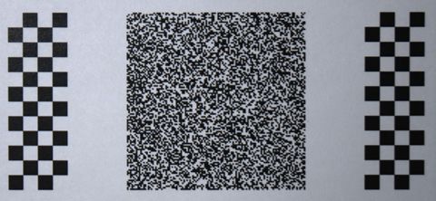
A. Optical Layer                                                       The PSF is dependent on the wavelength of the light source
   To simulate the system accurately, we model our system            and defocus. In the numerical simulations, the broadband color
based on Fourier optics theory [42], which takes account for         information in the training datasets — characterized as red (R),
diffraction and wavelength dependence. To keep the consis-           blue (B) and green (G) channels — are approximated by three
tency with natural lighting conditions, we assume that the light     discretized wavelengths, 610 nm (R), 530 nm (G) and 470 nm
source is incoherent.                                                (B), respectively.
   The optical layer simulates the working of a camera with                c) Coded image formulation: If the scene is comprised
a phase mask in its aperture plane. Given the phase mask,            of a planar object at a constant depth from the camera, the PSF
describes as a height map, we can first define the pupil function    is uniform over the image, and the image rendering process
induced by it, calculate the point spread function on the image      is just a simple convolution for each of the color channels.
plane and render the coded image produced by it given an             However, most real-world scenes contain depth variations, and
RGBD image input.                                                    the ensuing PSF is spatially varying. While there are plenty of
      a) Pupil function: Since the phase mask is placed on the       algorithms to simulate the depth-of-field effect [44]–[46], we
aperture plane, the pupil function is the direct way to describe     require four fundamental properties to be satisfied. First, the
the forward model. The pupil function is a complex-valued            rendering process has to be physically accurate and not just
function of the 2D coordinates (x1 , y1 ) describing the aperture    photo-realistic. Second, it should have the ability to model
plane.                                                               arbitrary phase masks and the PSF induced by them, rather
                                                                     than assuming a specific model on the PSF (e.g., Gaussian
            P (x1 , y1 ) = A(x1 , y1 ) exp[iφ(x1 , y1 )]      (1)
                                                                     distribution). Third, since the blurring process will be one
  The amplitude A(·, ·) is constant within the disk aperture         part of the end-to-end framework, it has to be differentiable.
and zero outside since there is no amplitude attenuation for         Fourth, this step should be computationally efficient because
phase masks. The phase φ has two components from the phase           the rendering process needs to be done for each iteration with
mask and defocus.                                                    updated PSFs.
                                                                        Our method is based on the layered depth of field model
           φ(x1 , y1 ) = φM (x1 , y1 ) + φDF (x1 , y1 )       (2)    [45]. The continuous depth map is discretized based on Wm .
                                                                     Each layer is blurred by its corresponding PSF calculated from
   φM (x1 , y1 ) is the phase modulation caused by height vari-
                                                                     (6) with a convolution. Then, the blurred layers are composited
ation on the mask.
                                                                     together to form the image.
                φM (x1 , y1 ) = kλ ∆n h(x1 , y1 )             (3)                        X
                                                                        IλB (x2 , y2 ) =     S
                                                                                            Iλ,Wm
                                                                                                  (x2 , y2 ) ⊗ P SFλ,Wm (x2 , y2 ) (7)
λ is the wavelength, kλ = 2π    λ is the wave vector, and ∆n is
                                                                                      Wm
the reflective index difference between air and the material of      This approach does not model the occlusion and hence, the
the phase mask. The material used for our phase mask has             rendered image is not accurate near the depth boundaries due
little refractive index variations in the visible spectrum [43];     to intensity leakage; however, for the most part, it does capture
so, we keep ∆n as a constant. h denotes the height map of            the out-of-focus effect correctly. We will discuss fine-tuning
the mask, which is what we need to learn in the optical layer.       of this model to reduce the error at boundaries in Section V-D.
    The term φDF (x1 , y1 ) is the defocus aberration due to the        To mimic noise during the capture, we apply Gaussian
mismatch between in-focus depth z0 and the actual depth z            noise to the image. A smaller noise level will improve the
of a scene point. The analytical expression for φDF (x1 , y1 ) is    performance during the reconstruction but also makes the
given as [42]                                                        model to be more sensitive to noise. In our simulation, we
                      x21 + y12 1                                    set the standard deviation σ = 0.01.

    DF                                 1
  φ (x1 , y1 ) = kλ                 −       = kλ Wm r(x1 , y1 )2 ,
                          2       z    z0
                                                               (4)
                     p                                                B. Depth Reconstruction Network
where r(x1 , y1 ) = x21 + y12 /R is the relative displacement,
R is the radius of the lens aperture, and Wm is defined as              There are a variety of networks to be applied for our depth
                                                                     estimation task. Here, we adopt the U-Net [47] since it is
                              R2 1

                                          1                          widely used for pixel-wise prediction.
                     Wm =             −       .                (5)
                               2    z    z0                             The network is illustrated in Figure 1, which is an encoder-
Wm combines the effect from the aperture size and the depth          decoder architecture. The input to the network is the coded
range, which is a convenient indication of the severity of the       image with three color channels. The encoder part consists
focusing error. For depths that are closer to the camera than        of the repeated application of two 3 × 3 convolutions, each
the focal plane, Wm is positive. For depths that are further         followed by a rectified linear unit (ReLU) and a batch nor-
than the focal plane, Wm is negative.                                malization (BN) [48]. At each downsampling step, we halve
     b) PSF induced by the phase mask: For an incoherent             the resolution using a 2 × 2 max pooling operation with stride
system, the PSF is the squared magnitude of the Fourier              2 and double the number of feature channels. The decoder part
transform of the pupil function.                                     consists of an upsampling of the feature map followed by a
                                                                     2 × 2 convolution that halves the number of feature channels
                                                          2
         P SFλ,Wm (x2 , y2 ) = |F{Pλ,Wm (x1 , y1 )}|          (6)    and two 3 × 3 convolutions, each followed by a ReLU and a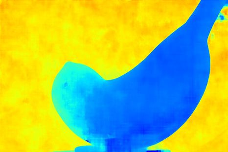
BN. Concatenation is applied between the encoder and decoder         The Fisher information matrix, which is a 3 × 3 matrix in
to avoid the vanishing gradient problem. At the final layer, a       our application, is given as
1x1 convolution is used with a sigmoid to map each pixel to                     Np
the given depth range.                                                          X         1         ∂P SFθ (t)      ∂P SFθ (t)
                                                                      Iij (θ) =                                                  ,
   During the training, the input image size is 256 × 256. But                  t=1
                                                                                    P SFθ (t) + β       ∂θi             ∂θj
the depth estimation network can be run fully-convolutionally                                                                (11)
for images size of any multiple of 16 at test time.                  where P SFθ (t) is the PSF intensity value at pixel t, Np
                                                                     is the number of pixels in the PSF, and θ = (x, y, z)
                                                                     corresponds to the 3D location.
    C. Loss Function
                                                                     The diagonal of the inverse of the Fisher information matrix
   Instead of optimizing depth z directly, we optimize Wm            yields the CRLB vector, which bounds the variance of the
which is linear to the inverse of the depth. Intuitively, since      3D location.
defocus blur is proportional to the inverse of the depth,                                                   h
                                                                                                                   −1
                                                                                                                      i
estimating depth directly would be highly unstable since even a            CRLBi ≡ σi 2 = E(θ̂i − θi )2 ≥ (I(θ))             (12)
                                                                                                                        ii
small perturbation in defocus blur estimation could potentially
                                                                     Finally, the loss is a summation of CRLB for different
lead to an arbitrarily large change in depth. Further, since
                                                                     directions, different depths, and different colors.
Wm is relative to the depth of the focus plane, it removes
                                                                                       X X X p
an additional degree of freedom that would otherwise need to              LCRLB =                           CRLBi (z, c) (13)
be estimated. Once we estimate Wm , the depth map can be                             i=x̂,ŷ,ẑ z∈Z c=R,G,B
calculated using (5).
                                                                     In theory, smaller LCRLB indicates better 3D localization.
   We use a combination of multiple loss functions
       Ltotal = λRM S LRMS + λgrad Lgrad + λCRLB LCRLB       (8)    D. Training / Implementation Details
Empirically, we found that setting the weights of the respective      We describe key elements of the training procedure used to
loss functions (if included) as λRM S = 1, λgrad = 1, and          perform the end-to-end optimization of the phase mask and
λCRLB = 1e−4 generates good results. We describe each loss         reconstruction algorithm.
function in detail.                                                      a) Basis for height maps: Recall that the phase mask is
• Root Mean Square (RMS). In order to force the estimated          described in terms of a height map. We describe the height map
  W
  cm to be similar to the ground truth Wm , we define a loss       at a resolution of 23 × 23 pixels. To speed up the optimization
  term using the RMS error.                                        convergence, we constrain the height map further by modeling
                                                                   it using the basis of Zernike polynomials [50]; this approach
                            1                                      was used previously by [49]. Specifically, we constrain the
                    LRMS = √ kWm − W
                                   cm k2 ,                   (9)
                            N                                      height map to the of the form
    where N is the number of pixels.                                                              55
                                                                                                  X
•   Gradient. In a natural scene, it is common to have multiple                       h(x, y) =         aj Zj (x, y)           (14)
    objects located at different depths, which creates sharp                                      j=1
    boundaries in the depth map. To emphasize the network
                                                                   where {Zj (x, y)} is the set of Zernike polynomials. The
    to learn these boundaries, we introduce an RMS loss on the
                                                                   goal now is to find the optimal coefficient vector a1×55 that
    gradient along both x and y directions.
                                                                   represents the height map of the phase mask.
                                                        !                b) Depth range: We choose the range of kG Wm to
                1      ∂Wm   ∂W
                              cm   ∂Wm   ∂W
                                          cm                       be [−10.5, 10.5]. The term kG is the wave vector for green
     Lgrad   = √           −     +     −                    (10)
                N       ∂x    ∂x    ∂y    ∂y                       wavelength (kG = λ2πG ; λG = 530nm) and we choose the
                                                                   range of kG Wm so that the defocus phase φDF is within a
•   Cramér-Rao Lower Bound (CRLB). The effectiveness of           practical range, as calculated by (4). For the remainder of the
    depth-varying PSF to capture the depth information can         paper, we will refer to kG Wm as the normalized Wm .
    be expressed using a statistical information theory measure       During the image rendering process, Wm needs to be dis-
    called the Fisher information. Fisher information provides     cretized so that the clean image is blurred layer by layer. There
    a measure of the sensitivity of the PSF to changes in          is a tradeoff between the rendering accuracy and speed. For
    the 3D location of the scene point [49]. Using the Fisher      the training, we discretize normalized Wm to [−10 : 1 : 10],
    information function, we can compute CRLB, which pro-          so that it has 21 distinct values.
    vides the fundamental bound on how accurately a parameter            c) Datasets: As discussed in the framework, our input
    (3D location) can be estimated given the noisy measure-        data requires both texture and depth information. The NYU
    ments. In our problem setting, the CRLB provides a scene-      Depth dataset [51] is a commonly used RGBD dataset for
    independent characterization of our ability to estimate the    depth-related problems. However, since Kinect captures the
    depth map. Prior work on 3D microscopy [49] has shown          ground-truth depth map, the dataset has issues in boundary
    that optimizing a phase mask using CRLB as the loss            mismatch and missing depth. Recently, synthetic data has been
    function provides diverse PSFs for different depths.           applied to geometric learning tasks because it is fast and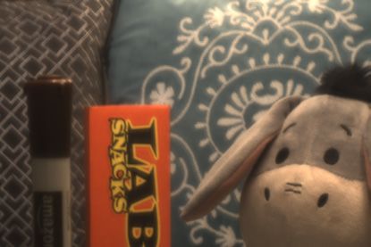
TABLE I                                 A. Ablation Studies
         Q UANTITATIVE E VALUATION OF A BLATION STUDIES
                                                                      To clearly understand our end-to-end system as well as
 Exp.   Learn mask   Initialization      Loss        Error (RMS)   choosing the correct parameters in our design space, we carry
  A         No         No mask           RMS             2.69
  B         Yes        Random            RMS             1.07      out several ablation experiments. We discuss our findings
  C         No       Fisher mask         RMS             0.97      below, provide quantitative results in Table I and the quali-
  D         Yes        Random          RMS+CRLB          0.88      tative visualizations in Figure 3. For convenience, we use the
  E         Yes      Fisher mask         RMS             0.74
  F         Yes      Fisher mask       RMS+CRLB          0.85      numbering in the first column of Table I when referring to the
  G         Yes      Fisher mask      RMS+gradient       0.56      experiment performed and the corresponding models acquired
                                                                   in the ablation study. For all the experiments here, we use
                                                                   the same U-Net architecture as discussed in Section III-B for
                                                                   depth reconstruction. The baseline for all comparison is model
cheap to produce and contains precise texture and depth. We        (A), a depth-reconstruction-only network trained with a fixed
use FlyingThings3D from Scene Flow Datasets [40], which            open aperture and RMS loss.
includes both all-in-focus RGB images and corresponding
                                                                         a) Learned vs. fixed mask: In this first experiment,
disparity map for 2247 training scenes. Each scene contains
                                                                   we use our end-to-end framework to learn both the phase
ten successive frames. We used the first and last frames in
                                                                   mask and the reconstruction layer parameters from randomly
each sequence to avoid redundancies.
                                                                   initialized values (Exp. B). For comparison, we have Exp. C
   To accurately generate 256 × 256 coded images using PSFs        where the phase mask is fixed to the Fisher mask, which is
of size 23 × 23 pixels, we need all-in-focus images at a           designed by minimizing LCRLB in our depth range, and we
resolution 278×278 pixels. We generate such data by cropping       learn only the reconstruction layer from random initialization.
patches of appropriate size from the original images (whose
                                                                      To our surprise, shown in Table I and Figure 3 (Exp. B vs.
resolution is 960 × 540) with a sliding window of 200 pixels.
                                                                   C), when learning from scratch (random phase mask param-
We only select the image whose disparity map ranges from 3
                                                                   eters), our end-to-end learned masks (B) underperforms the
to 66 pixels and convert them to Wm linearly.
                                                                   Fisher mask that was designed using a model-based approach
   With this pre-processing, we obtain 5077 training patches,      (C). We believe that there are two insights to be gained from
553 validation patches, and 419 test patches. The data is          this observation. First, the CRLB cost is very powerful by itself
augmented with rotation and flip, as well as brightness scaling    and leads to a phase mask that is well suited for depth estima-
randomly between 0.8 to 1.1.                                       tion; this is expected given the performance of prior work that
     d) Training process: Given the forward model and the          exploits the CRLB cost. Second, a random initialization fails
loss function, the back-propagation error can be derived using     to converge to the desired solution in part due to the highly
the chain rule. In our system, the back-propagation is obtained    non-convex nature of the optimization problem and the undue
by the automatic differentiation implemented in TensorFlow         influence of the initialization. We visualize the corresponding
[52]. For those who are interested in the derivation for the       phase mask height map is visualized in Figure 4, where 4(a)
optical layer, please refer to our supplementary material.         is the mask learned from scratch in Exp. B, and 4(b) is the
During the training, we use Adam [53] optimizer with pa-           fixed Fisher in Exp. C.
rameters β1 = 0.99 and β2 = 0.999. Empirically, we found                 b) Effect of initialization conditions: With our hypothesis
that using different learning rates for the phase mask and depth   drawn from the previous experiment, we explore if careful
reconstruction improves the performance. We suspect this is        initialization would help in improving overall performance.
due to the large influence that the phase mask has on the U-       Instead of initializing with random values in Exp. B, we
Net given that even small changes to the mask produces large       initialize the mask as a Fisher mask in Exp. E, and perform
changes in the coded image. In our simulation, the learning        end-to-end optimization of both the mask design and the
rates for phase mask and depth reconstruction were 10−8 and        reconstruction network (there is no constraint forcing the
10−4 , respectively. A learning rate decay of 0.1 was applied      optical network to generate masks that are close to the Fisher
at 10K and 20K iterations. We observed that the training           mask). Interestingly, under such an initialization, the end-to-
converges after about 30K iterations. We used a training mini-     end optimization improves the performance compared to the
batch size to be 40. Finally, the training and testing were        randomly initialized mask (B) by a significant margin (1.07
performed on NVIDIA Tesla K80 GPUs.                                vs. 0.74 in RMS), and it also out-performs the fixed Fisher
                                                                   mask (Exp. C) noticeably (0.97 vs. 0.74 in RMS), suggesting
                                                                   the CRLB-model-based mask design can be further improved
                      IV. S IMULATION                              by data-driven fine-tuning. This is reasonable given that the
                                                                   model-based mask design does not optimize directly on the
   The end-to-end framework learns the phase mask design and       end objective – namely, a high-quality precise depth map
reconstruction algorithm in the simulation. In this section, We    that can capture both depth discontinuities and smooth depth
perform ablation studies to identify elements that contribute      variations accurately. Fisher mask is the optimal solution for
most to the overall performance as well as identify the best       3D localization when the scene is sparse [49]. However, most
operating point. Finally, we provide comparisons with other        real-world scenes are not sparse and hence optimizing for the
depth estimation methods using simulations.                        actual depth map allows us to beat the performance of the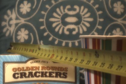
No mask        Random initialized mask   Fisher fixed mask   Random initialized mask Fisher initialized mask Fisher initialized mask Fisher initialized mask
                    Ground truth   RMS loss (A)        RMS loss (B)            RMS loss (C)       RMS+CRLB loss (D)          RMS loss (E)        RMS+CRLB loss (F)        RMS+grad loss (G)
Coded images

                                                                                                                                                                                                   10
Disparity map

                                                                                                                                                                                                   5

                                                                                                                                                                                                   0

                                                                                                                                                                                                   -5

                                                                                                                                                                                                   -10

                Avg. RMS error:     2.69                   1.07                   0.97                    0.88                   0.74                    0.85                      0.56

Fig. 3. Qualitative results from our ablation studies. Across the columns, we show the inputs to the reconstruction network and the depth estimation
results from the network. The numbering A-G here correspond to the experiment setup A-G in Table I. The best result is achieved when we initialize the
optical layer with the phase mask derived using Fisher information and then letting the CNN further optimize the phase mask. The last column (G) shows
the results from our best phase mask.

                                                                                                       -10 (far)        -9            -8            -7           -6            -5            -4

                                                                                                           -3            -2           -1            0             1            2             3

                           (a)               (b)                      (c)
                                                                                                           4             5             6            7             8            9          10 (near)

Fig. 4. Phase mask height maps from ablation studies. (a) Trained from
random initialization with RMS loss. (b) Fisher initialized mask. (c) Trained
from Fisher initialization with RMS and gradient loss.

                                                                                                    Fig. 5. Simulated PSFs of our optimal phase mask. The PSFs are labeled
                                                                                                    in terms of Wm . Range −10 to 10 corresponds to the depth plane from far
                                                                                                    to near.
Fisher mask.
   The use of Fisher mask to initialize the network might raise                                       B. Operating Point with Best Performance
the concern whether the proposed approach is still end-to-                                             Figure 4(c) shows the best phase mask design based on
end. We believe the answer is positive, because initializing a                                      our ablation study. It shares some similarity with the Fisher
network from designed weights instead of from scratch is a                                          mask since we take the Fisher mask as our initialization.
common practice in deep learning (i.e., the Xavier approach                                         But our mask is further optimized based on the depth map
[54] and the He approach [55]). Likewise, here we incorporate                                       from our data. Figure 5 displays depth-dependent PSFs in
our domain knowledge and use a model-based approach in                                              the range [−10 : 1 : 10] of normalized Wm . These PSFs
designing the initialization condition of our optical layers.                                       have large variability across different depths for improving
      c) Effect of loss functions: Finally, we also test different                                  the performance of depth estimation. More simulation results
combinations of Losses discussed in Section III-C with the                                          are shown in Figure 6.
Fisher mask as the initialization (E, F, and G). We found
that RMS with gradient loss (G) gives the best results. For                                           C. Comparisons with the State-of-the-Art
completeness, we also show the performance of randomly                                                 We compare our result with state-of-the-art passive, single
initialized mask with RMS and CRLB loss in D.                                                       viewpoint depth estimation methods.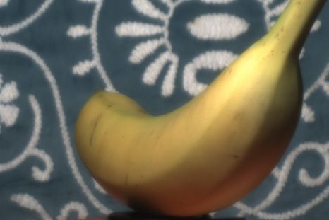
Levin et al. Veeraraghavan et al.
                                                                                           Ground truth                                        Ours
Clean images
                                                                                                               [1]              [3]

                                                                            Coded images
Coded images

                                                                                                                                                      10

                                                                           Disparity map
                                                                                                                                                      5

                                                                                                                                                      0

                                                                     10                                                                               -5
Est. disparity

                                                                     5                                                                                -10

                                                                     0

                                                                     -5
                                                                           Fig. 7. Depth estimation comparing with coded amplitude masks. Our
                                                                     -10   reconstructed disparity map achieves the best performance. Also, our system
                                                                     10    has higher light efficiency by using the phase mask. The scaled disparity map
True disparity

                                                                     5     have units in terms of normalized Wm .
                                                                     0

                                                                     -5
                                                                                                                  TABLE III
                                                                                                C OMPARISON WITH THE TWO - RING PHASE MASK [4]
                                                                     -10

                                                                                                            Method                   |Wm − Ŵm |
Fig. 6. Simulation results with our best phase mask. The reconstructed                           Two-ring mask + Haim’s network          0.6
disparity maps closely match the ground truth disparity maps. The scaled                             Two-ring mask + U-Net              0.51
disparity map have units in terms of normalized Wm .                                              Our Optimized Mask + U-Net            0.42

                                 TABLE II
                 C OMPARISON WITH A MPLITUDE M ASK DESIGN
                                                                                 c) Semantics-based single image depth estimation: To
                                                                           compare the performance of our proposed methods with other
                           Mask design           LRM S                     deep-learning-based depth estimation methods using a single
                          Levin et al. [1]        1.04
                      Veeraraghavan et al. [3]    1.08                     all-focus image, we run evaluation experiments on standard
                               Ours               0.56                     NYU Depth V2 datasets [51]. We used the default train-
                                                                           ing/testing splits provided by the datasets. The size of training
                                                                           and testing images are re-sized from 640 × 480 to 320 × 240
                                                                           following the data augmentations the common practice [29].
     a) Coded amplitude masks: There are two well-known                    We show the comparison of our proposed methods with other
amplitude masks for depth estimation. Levin et al. [1] design              state-of-the-art passive single image depth estimation results
a mask by maximizing the blurry image distributions from dif-              [29]–[35] in Table IV. We use the standard performance
ferent depths using Kullback-Leibler divergence. Veeraragha-               metrics used by all the aforementioned works for comparison,
van et al. [3] select the best mask by maximizing the minimum              including linear root mean square error (RMS), absolution
of the discrete Fourier transformation magnitudes of the zero              relative error (REL), logarithm-scale root mean square error
padded code. To make a fair comparison between their masks                 (Log10) and depth estimation accuracy within a threshold
and our proposed mask, we render blurry image datasets based               margin (δ within 1.25, 1.252 and 1.253 away from the ground
on each mask with the same noise level (σ = 0.01). Since U-                truth). We refer the readers to [29] for the detailed definitions
Net is a general pixel-wise estimation network, we use it with             of the metrics. As one can see, we achieve better performance
same architecture introduced in III-B for depth reconstruction.            in every metrics category for depth estimation error and
Parameters in the U-Net are learned for each dataset using                 accuracy, which suggests that the added end-to-end optimized
RMS and gradient loss.                                                     phase mask does help improve the depth estimation. Moreover,
   The quantitative results are shown in Table II and qualitative          we don’t have the issue of scaling ambiguity in depth like those
results are shown in Figure 7. Our proposed mask offers the                semantics based single-image depth estimation methods since
best result with the smallest RMS error. One key reason is that            our PSFs are based on absolute depth values.
these amplitude masks only change the scaling factor of PSF
at different depths, while our mask creates a more dramatic                          V. E XPERIMENTS ON R EAL H ARDWARE
difference in PSF at different depths.                                        We fabricate the phase masks learned through our end-to-
     b) Two-ring phase mask: Recently, Haim et al. [4] pro-                end optimization, and evaluated its performance on a range of
pose a two-ring phase mask for depth estimation. To compare                real-world scenes. The experiment details are discussed below,
the performance, we use their dataset “TAU-Agent” and the                  and the qualitative results are shown in Figure 11.
same parameters described in their paper. Performance is
evaluated by the L1 loss of Wm . As shown in Table III, both                 A. Experiment Setup
our reconstruction network and our phase mask contribute to                   In the experiment, we use a Yongnuo 50mm f /1.8 standard
achieving smallest estimation error.                                       prime lens, which is easy to access the aperture plane. The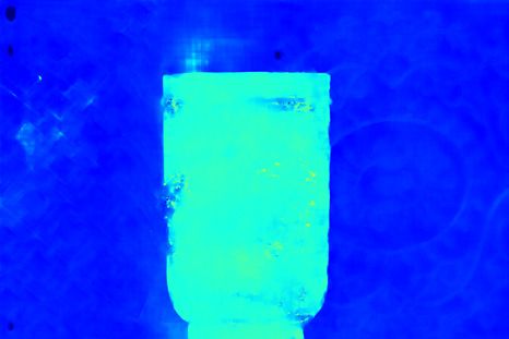
TABLE IV                                             -10 (1 m)              -9           -8         -7           -6              -5           -4
      C OMPARISON WITH SEMANTICS - BASED SINGLE IMAGE DEPTH
         ESTIMATION METHODS ON NYU D EPTH V2 DATASETS .

 Method                        Error                  Accuracy, δ <                  -3                -2           -1          0           1               2             3

                     RMS      REL      Log10       1.25    1.252       1.253
 Make3D [29]         1.214    0.349                0.447   0.745       0.897         4                 5            6           7           8               9       10 (0.4 m)
 Eigen [29]          0.907    0.215    -           0.611   0.887       0.971
 Liu [30]            0.824    0.23     0.095       0.614   0.883       0.971
 Cao [32]            0.819    0.232    0.091       0.646   0.892       0.968
 Chakrabarti [31]    0.620    0.149    -           0.806   0.958       0.987
 Qi [33]             0.569    0.128    0.057       0.834   0.96        0.99
 Laina [34]          0.573    0.127    0.055       0.811   0.953       0.988
                                                                               Fig. 9. Calibrated PSFs of the fabricated phase mask. The camera lens
 Hu [35]             0.530    0.115    0.050       0.866   0.975       0.993
                                                                               with the phase mask in its aperture is calibrated for depths 0.4 m to 1 m,
 Ours                0.382    0.093    0.050       0.932   0.989       0.997
                                                                               which corresponds to the normalized Wm range for an aperture size of 2.835
                                                                               mm.

  In-focus image with clean aperture           Image with phase mask             Naive rendering        Matting rendering           Experimental reconstruction
                                                                                                                            Coded image      Naive render        Matting render

Fig. 8. Calibration target for PSF estimation. An example of a sharp image     Fig. 10. Fine-tune digital network with matting-based rendering. (Left)
(left) taken using a camera lens without the phase mask and a coded image      Example comparison between naive rendering and matting-based rendering.
(right) taken through the phase mask. The checkerboard pattern around the      Without blending between the depth layers, the naive rendering show artifacts
calibration target is used for the alignment of the image pairs.               on depth boundaries as shown in the insets. The matting-based rendering is
                                                                               more realistic throughout the image. (Right) Improvement in depth estimation
                                                                               of real experimental data is observed when the digital network is fine-tuned
                                                                               with matting-based rendered training data. The improvement is visible along
sensor is a 5472 × 3648 machine vision color camera (BFS-                      the edges of the leaf.
PGE-200S6C-C) with 2.4 µm pixel size. We set the diameter
of the mask phase to be 2.835 mm. Thus, the simulated pixel
size is about 9.4 µm for the green channel, which corresponds                  phase mask aperture alignment. We adopted an optimization-
to 4 pixels in our actual camera. For each 4 × 4 region, we                    based approach where we estimate the PSFs from a set of sharp
group it to be one pixel with RGB channels by averaging each                   and coded image pairs [57], [58] of a calibration pattern.
color channel based on the Bayer pattern, therefore the final                     Estimating the PSF can be posed as a deconvolution prob-
output resolution of our system is 1344 × 894.                                 lem, where both a sharp image and a coded image of the same
                                                                               calibration target are given. The calibration target we used is a
                                                                               random binary pattern that was laser-printed on paper. We used
  B. Phase Mask Fabrication                                                    two identical camera lenses, one without the phase mask to
   The size of the designed phase mask is 21 × 21, with each                   capture the sharp image and the other with the phase mask in
grid corresponding to a size of 135 µm × 135 µm. The full                      the aperture to capture the coded image. Image pairs are then
size of the phase mask is 2.835 mm × 2.835 mm.                                 obtained for each depth plane of interest. The lens focus was
   The phase mask was fabricated using two-photon lithog-                      adjusted at every depth plane to capture sharp images while
raphy 3D printer (Photonic Professional GT, Nanoscribe                         the focus of the camera lens with the phase mask was kept
GmbH [56]). For a reliable print, the height map of the                        fixed. Checkerboard pattern was used around the calibration
designed phase mask was discretized into steps of 200 nm. The                  pattern to assist in correcting for any misalignment between
phase mask was printed on a 170 µm thick, 30 mm diameter                       the sharp and the coded image.
glass substrate using Nanoscribe’s IP-L 780 photoresist in                        For a particular depth plane, let I be the sharp image
a direct laser writing configuration with a 63× microscope                     and J be the coded image taken using the phase mask. We
objective lens. The glass substrate was then cut to a smaller                  can estimate the PSF popt by solving the following convex
size to fit into the camera lens’ aperture. Close-up of the phase              optimization problem
mask in the camera lens aperture is shown in Figure 2.                                                                         2                                                  2
                                                                               popt = argmin kI ∗ p − s · Jk2 + λ k∇pk1 + µ 1T p − 1                                              2
                                                                                                   p
                                                                                                                                       (15)
  C. PSF Calibration
                                                                               where the first term is a least-squares data fitting
   Although the depth-dependant PSF response of the phase                      term
                                                                               P                P convolution), and the scalar s =
                                                                                       (‘∗’ denotes
mask is known from simulation, we calibrate our prototype                         m,n  I(m, n)/   m,n J(m, n) normalizes the difference in
camera to account for any mismatch born out of physical im-                    exposure between the image pairs. The second term con-
plementation such as aberrations in fabricated phase mask and                  straints the gradients of the PSF to be sparse and the third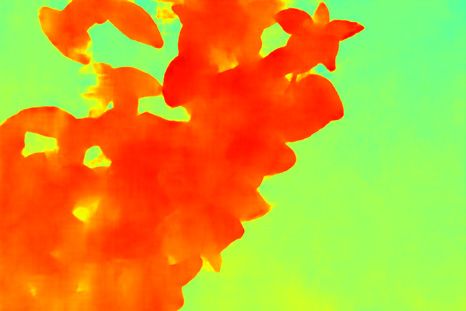
Indoor scenes                                                               Outdoor scenes
                 A                                B                                  C                                          D
 Coded images

                                                                                                                                                                 10
 Disparity map

                                                                                                                                                                 5

                                                                                                                                                                 0

                                                                                                                                                                 -5

                                                                                                                                                                 -10
                 E                                F                                  G                                          H
 Coded images
 Depth map

                         0.4    0.5   0.6       0.7     0.8     0.9   1                           0.5   0.6   0.7   0.8   0.9       1   1.1   1.2    1.3   1.4
                                              meters                                                                      meters

Fig. 11. Real-world results. Results of various scenario are shown and compared: Indoor scenes (A, B, E, and F) are shown on the left and outdoor scenes
(C, D, G, and H) are on the right; Smoothly changing surfaces are presented in (A, D and F) and sharp object boundaries in (B, C, E, G, and H); Special
cases of a transparent object (B) and texture-less areas (E and F) are also included.

                     Coded images           Estimated depth by PhaseCam3D           Estimated depth by Kinect
                                                                            1.4

                                                                            1.2

                                                                            1 [m]

                                                                            0.8

                                                                            0.6

                                                          (a)                                                                                       (b)

Fig. 12. Validation experiments. (a) Comparison with the Microsoft Kinect V2. (b) Depth accuracy evaluation of PhaseCam3D by capturing targets at
known depths. The actual depth is measured by a tape measure.
term enforces an energy conservation constraint. The above VI. C ONCLUSION
optimization problem can be solved using first-order primal- In this work, we apply phase mask to the aperture plane
dual algorithm presented in [58], [59]. The PSF estimation of a camera to help estimate the depth of the scene and
is performed for each color channel and each depth plane use a novel end-to-end approach to design the phase mask
independently. and the reconstruction algorithm jointly. In our end-to-end
framework, we model the optics as learnable neural network
D. Fine-tuning the Digital Network layers and connected them to the consequent reconstruction
layers for depth estimation. As a result, we are able to use
When training for phase mask profile using our framework, back-propagation to optimize the reconstruction layers and the
we used naive rendering to simulate the coded image as optics layers end-to-end. Compared to existing depth estima-
described in Section III-A(c). Such a rendering process is fast, tion methods, such as stereo vision and ToF sensors, our phase
allowing for multiple cycles of rendering and sufficient to ex- mask-based approach uses only single-shot, single-viewpoint
plain most out-of-focus regions of the scene. However, without and requires no specialty light source, making it easy to
blending between the depth layers, the naive rendering is not set up, suitable for dynamic scenes, consumes less energy
realistic at depth boundaries. Hence, the digital reconstruction and robust to any lighting condition. Following our proposed
network trained using naive rendering shows artifacts at object framework, we build a prototype depth estimation camera
boundaries as shown in Figure 10. using the end-to-end optimized phase mask and reconstruction
To improve the performance of the depth reconstruction network. The fabrication of the phase mask is low cost and
network, we fix the optimized phase mask and retrain the can be easily scaled up for mass production. Looking into the
digital network with a matting-based rendering technique [60]. future, we hope to extend our framework to more applications,
Matting for each depth layer was computed by convolving such as microscopy. We also are interested in modeling other
the corresponding PSF with the depth layer mask. The coded components in the imaging system (i.e. ISP pipeline, lenses,
image was then composited, ordered from farther blurred lay- and spectral filters) in our end-to-end framework, so as to aim
ers to nearer blurred layers. The layers were linearly blended for a more completely optimized the camera for higher-level
using the normalized matting weights [61]. Since the PSFs computer vision tasks.
are fixed, rendering of all the coded imaged can be created
apriori and fed into the training of the depth reconstruction ACKNOWLEDGMENT
network. The use of closer-to-reality matting-based rendering
improved our experimental reconstructions significantly at the This work was supported in part by NSF grants IIS-
object boundaries, as shown in Figure 10. 1652633, IIS-1618823, CCF-1527501, CCF-1730574, CCF-
1652569 and DARPA NESD program HR0011-17-C-0026. Y.
W. was partially supported by Information Technology Oil
E. Real-world Results & Gas HPC Conference Graduate Fellowship from the Ken
Using the hardware prototype we built, we acquire the depth Kennedy Institute.
of the real world scenes. We show the results in Figure 11.
As one can observe, our system is robust to lighting condition R EFERENCES
as reasonable depth estimation for both indoor scenes (A, B, [1] A. Levin, R. Fergus, F. Durand, and W. T. Freeman, “Image and depth
E, and F) and outdoor scene (C, D, G, and H) are produced. from a conventional camera with a coded aperture,” ACM Transactions
on Graphics (TOG), vol. 26, no. 3, p. 70, 2007.
Both smoothly changing surface (A, D and F) and sharp object [2] C. Zhou, S. Lin, and S. K. Nayar, “Coded aperture pairs for depth from
boundaries (B, C, E, G, and H) are nicely portrayed. Special defocus and defocus deblurring,” International Journal of Computer
cases of a transparent object (B) and texture-less areas (E and Vision, vol. 93, no. 1, pp. 53–72, 2011.
[3] A. Veeraraghavan, R. Raskar, A. Agrawal, A. Mohan, and J. Tumblin,
F) are also nicely handled. “Dappled photography: Mask enhanced cameras for heterodyned light
In addition, given the Microsoft Kinect V2 [15] is the fields and coded aperture refocusing,” ACM Transactions on Graphics
one of the best ToF-based depth camera available on the (TOG), vol. 26, no. 3, p. 69, 2007.
[4] H. Haim, S. Elmalem, R. Giryes, A. Bronstein, and E. Marom, “Depth
mainstream market, we show our depth estimation results Estimation from a Single Image using Deep Learned Phase Coded
against the Kinect results in Figure 12(a). As one can see, Mask,” IEEE Transactions on Computational Imaging, vol. 4, no. 3,
the Kinect indeed output smoother depth on flat surfaces than pp. 298–310, 2018.
[5] A. Chakrabarti, “Learning sensor multiplexing design through back-
our system, however, our method handles the depth near the propagation,” in Advances in Neural Information Processing Systems,
object boundary better than Kinect. 2016.
To validate the depth-reconstruction accuracy of our pro- [6] V. Sitzmann, S. Diamond, Y. Peng, X. Dun, S. Boyd, W. Heidrich,
F. Heide, and G. Wetzstein, “End-to-end optimization of optics and
totype, we captured a planar target placed at various known image processing for achromatic extended depth of field and super-
depths. We compute the depth of the target and then compare resolution imaging,” ACM Transactions on Fraphics (TOG), vol. 37,
against the known depths. As shown in Figure 12(b), we no. 4, pp. 1–13, 2018.
[7] D. Gabor, “A new microscopic principle,” 1948.
reliably estimate the depth throughout the entire range. [8] Y. N. Denisyuk, “On the reflection of optical properties of an object in
For comparison, we also tested the Fisher mask in exper- a wave field of light scattered by it,” Doklady Akademii Nauk SSSR, vol.
iments. The results show that our proposed mask provides 144, no. 6, pp. 1275–1278, 1962.
[9] E. N. Leith and J. Upatnieks, “Reconstructed wavefronts and commu-
better depth estimation. Detailed description can be found in nication theory,” Journal of the Optical Society of America A (JOSA),
the supplementary material. vol. 52, no. 10, pp. 1123–1130, 1962.[10] “Holokit hologram kits,” https://www.integraf.com/shop/hologram-kits. [40] N. Mayer, E. Ilg, P. Hausser, P. Fischer, D. Cremers, A. Dosovitskiy, and
[11] “Liti holographics litiholo kits,” https://www.litiholo.com/. T. Brox, “A large dataset to train convolutional networks for disparity,
[12] T. Tahara, X. Quan, R. Otani, Y. Takaki, and O. Matoba, “Digital optical flow, and scene flow estimation,” in CVPR, 2016.
holography and its multidimensional imaging applications: a review,” [41] A. Geiger, P. Lenz, C. Stiller, and R. Urtasun, “Vision meets robotics:
Microscopy, vol. 67, no. 2, pp. 55–67, 2018. The kitti dataset,” the International Journal of Robotics Research,
[13] J. Geng, “Structured-light 3d surface imaging: a tutorial,” Advances in vol. 32, no. 11, pp. 1231–1237, 2013.
Optics and Photonics, vol. 3, no. 2, pp. 128–160, 2011. [42] J. W. Goodman, Introduction to Fourier Optics. Roberts and Company
[14] S. Foix, G. Alenya, and C. Torras, “Lock-in time-of-flight (tof) cameras: Publishers, 2005.
A survey,” IEEE Sensors Journal, vol. 11, no. 9, pp. 1917–1926, 2011. [43] T. Gissibl, S. Wagner, J. Sykora, M. Schmid, and H. Giessen, “Refractive
[15] Z. Zhang, “Microsoft kinect sensor and its effect,” IEEE Multimedia, index measurements of photo-resists for three-dimensional direct laser
vol. 19, no. 2, pp. 4–10, 2012. writing,” Optical Materials Express, vol. 7, no. 7, pp. 2293–2298, 2017.
[16] M. Gupta, A. Agrawal, A. Veeraraghavan, and S. G. Narasimhan, [44] B. Barsky and T. J. Kosloff, “Algorithms for Rendering Depth of
“Structured light 3d scanning in the presence of global illumination,” Field Effects in Computer Graphics,” World Scientific and Engineering
in CVPR, 2011. Academy and Society (WSEAS), pp. 999–1010, 2008.
[17] N. Matsuda, O. Cossairt, and M. Gupta, “Mc3d: Motion contrast 3d [45] C. Scofield, “212-d depth-of-field simulation for computer animation,”
scanning,” in IEEE International Conference on Computational Pho- in Graphics Gems III (IBM Version), 1992.
tography (ICCP), 2015. [46] M. Kraus and M. Strengert, “Depth-of-field rendering by pyramidal
[18] S. Achar, J. R. Bartels, W. L. Whittaker, K. N. Kutulakos, and S. G. image processing,” Computer Graphics Forum, vol. 26, no. 3, pp. 645–
Narasimhan, “Epipolar time-of-flight imaging,” ACM Transactions on 654, 2007.
Graphics (TOG), vol. 36, no. 4, p. 37, 2017. [47] O. Ronneberger, P. Fischer, and T. Brox, “U-net: Convolutional networks
[19] R. Hartley and A. Zisserman, Multiple View Geometry in Computer for biomedical image segmentation,” in International Conference on
Vision. Cambridge university press, 2003. Medical Image Computing and Computer-assisted Intervention, 2015.
[20] D. Scharstein, H. Hirschmüller, Y. Kitajima, G. Krathwohl, N. Nešić, [48] S. Ioffe and C. Szegedy, “Batch normalization: Accelerating deep
X. Wang, and P. Westling, “High-resolution stereo datasets with network training by reducing internal covariate shift,” arXiv:1502.03167,
subpixel-accurate ground truth,” in German Conference on Pattern 2015.
Recognition, 2014. [49] Y. Shechtman, S. J. Sahl, A. S. Backer, and W. E. Moerner, “Optimal
[21] “Light l16 camera,” https://www.light.co/camera. point spread function design for 3D imaging,” Physical Review Letters,
[22] G. Neukum, R. Jaumann, H. Hoffmann, E. Hauber, J. Head, vol. 113, no. 3, pp. 1–5, 2014.
A. Basilevsky, B. Ivanov, S. Werner, S. Van Gasselt, J. Murray et al., [50] M. Born and E. Wolf, Principles of Optics: Electromagnetic Theory of
“Recent and episodic volcanic and glacial activity on mars revealed by Propagation, Interference and Diffraction of Light. Elsevier, 2013.
the high resolution stereo camera,” Nature, vol. 432, no. 7020, p. 971, [51] N. Silberman, D. Hoiem, P. Kohli, and R. Fergus, “Indoor segmentation
2004. and support inference from rgbd images,” in European Conference on
Computer Vision, 2012.
[23] C. Tomasi and T. Kanade, “Shape and motion from image streams under
[52] M. Abadi, P. Barham, J. Chen, Z. Chen, A. Davis, J. Dean, M. Devin,
orthography: a factorization method,” International Journal of Computer
S. Ghemawat, G. Irving, M. Isard et al., “Tensorflow: a system for large-
Vision, vol. 9, no. 2, pp. 137–154, 1992.
scale machine learning.” in Symposium on Operating Systems Design
[24] J. Sun, Y. Li, S. B. Kang, and H.-Y. Shum, “Symmetric stereo matching
and Implementation (OSDI), 2016.
for occlusion handling,” in CVPR, 2005.
[53] D. P. Kingma and J. Ba, “Adam: A method for stochastic optimization,”
[25] C. L. Zitnick and T. Kanade, “A cooperative algorithm for stereo match-
arXiv:1412.6980, 2014.
ing and occlusion detection,” IEEE Transactions on Pattern Analysis and
[54] X. Glorot and Y. Bengio, “Understanding the difficulty of training
Machine Intelligence, vol. 22, no. 7, pp. 675–684, 2000.
deep feedforward neural networks,” in the International Conference on
[26] A. F. Bobick and S. S. Intille, “Large occlusion stereo,” International
Artificial Intelligence and Statistics, 2010.
Journal of Computer Vision, vol. 33, no. 3, pp. 181–200, 1999.
[55] K. He, X. Zhang, S. Ren, and J. Sun, “Delving deep into rectifiers:
[27] Q. Yang, C. Engels, and A. Akbarzadeh, “Near real-time stereo for Surpassing human-level performance on imagenet classification,” in
weakly-textured scenes.” in British Machine Vision Conference, 2008. International Conference on Computer Vision, 2015.
[28] K. Konolige, “Projected texture stereo,” in Robotics and Automation, [56] “Nanoscribe gmbh,” https://www.nanoscribe.de/.
2010. [57] L. Yuan, J. Sun, L. Quan, and H.-Y. Shum, “Image deblurring with
[29] D. Eigen, C. Puhrsch, and R. Fergus, “Depth map prediction from a blurred/noisy image pairs,” ACM Transactions on Graphics (TOG),
single image using a multi-scale deep network,” in Advances in Neural vol. 26, no. 3, p. 1, 2007.
Information Processing Systems, 2014. [58] F. Heide, M. Rouf, M. B. Hullin, B. Labitzke, W. Heidrich, and
[30] F. Liu, C. Shen, and G. Lin, “Deep convolutional neural fields for depth A. Kolb, “High-quality computational imaging through simple lenses,”
estimation from a single image,” in CVPR, 2015. ACM Transactions on Graphics (TOG), vol. 32, no. 5, pp. 1–14, 2013.
[31] A. Chakrabarti, J. Shao, and G. Shakhnarovich, “Depth from a single [59] A. Chambolle and T. Pock, “A first-order primal-dual algorithm for
image by harmonizing overcomplete local network predictions,” in convex problems with applications to imaging,” Journal of Mathematical
Advances in Neural Information Processing Systems, 2016. Imaging and Vision, vol. 40, no. 1, pp. 120–145, 2011.
[32] Y. Cao, Z. Wu, and C. Shen, “Estimating depth from monocular images [60] M. Kraus and M. Strengert, “Depth-of-field rendering by pyramidal
as classification using deep fully convolutional residual networks,” IEEE image processing,” in Computer Graphics Forum, 2007.
Transactions on Circuits and Systems for Video Technology, vol. 28, [61] S. Lee, G. J. Kim, and S. Choi, “Real-time depth-of-field rendering using
no. 11, pp. 3174–3182, 2018. point splatting on per-pixel layers,” in Computer Graphics Forum, 2008.
[33] X. Qi, R. Liao, Z. Liu, R. Urtasun, and J. Jia, “Geonet: Geometric neural
network for joint depth and surface normal estimation,” in CVPR, 2018.
[34] I. Laina, C. Rupprecht, V. Belagiannis, F. Tombari, and N. Navab,
“Deeper depth prediction with fully convolutional residual networks,”
in 3D Vision (3DV), 2016.
[35] J. Hu, M. Ozay, Y. Zhang, and T. Okatani, “Revisiting single image
depth estimation: Toward higher resolution maps with accurate object
boundaries,” arXiv:1803.08673, 2018.
[36] R. Garg, V. K. BG, G. Carneiro, and I. Reid, “Unsupervised cnn for
single view depth estimation: Geometry to the rescue,” in European
Conference on Computer Vision, 2016.
[37] C. Godard, O. Mac Aodha, and G. J. Brostow, “Unsupervised monocular
depth estimation with left-right consistency,” in CVPR, 2017.
[38] T. Zhou, M. Brown, N. Snavely, and D. G. Lowe, “Unsupervised
learning of depth and ego-motion from video,” in CVPR, 2017.
[39] B. Ummenhofer, H. Zhou, J. Uhrig, N. Mayer, E. Ilg, A. Dosovitskiy,
and T. Brox, “Demon: Depth and motion network for learning monocular
stereo,” in CVPR, 2017.You can also read