Learning a Functional Control for High-Frequency Finance
←
→
Page content transcription
If your browser does not render page correctly, please read the page content below
Learning a Functional Control
                                                                for High-Frequency Finance
arXiv:2006.09611v2 [math.OC] 12 Feb 2021

                                                                  L. LEAL,† M. LAURIERE,† C.-A. LEHALLE‡

                                                 †
                                                  Department of Operations Research and Financial Engineering, Princeton University,
                                                                                Princeton, NJ - 08544
                                                                           {lleal,lauriere}@princeton.edu
                                           ‡
                                               Capital Fund Management, Paris, and Imperial College, London. 23 rue de l’Université, 75007
                                                                                     Paris, France
                                                                            charles-albert.lehalle@cfm.fr

                                           We use a deep neural network to generate controllers for optimal trading on high frequency data. For
                                           the first time, a neural network learns the mapping between the preferences of the trader, i.e. risk
                                           aversion parameters, and the optimal controls. An important challenge in learning this mapping is that,
                                           in intra-day trading, trader’s actions influence price dynamics in closed loop via the market impact. The
                                           exploration–exploitation tradeoff generated by the efficient execution is addressed by tuning the trader’s
                                           preferences to ensure long enough trajectories are produced during the learning phase. The issue of
                                           scarcity of financial data is solved by transfer learning: the neural network is first trained on trajectories
                                           generated thanks to a Monte-Carlo scheme, leading to a good initialization before training on historical
                                           trajectories. Moreover, to answer to genuine requests of financial regulators on the explainability of
                                           machine learning generated controls, we project the obtained “blackbox controls” on the space usually
                                           spanned by the closed-form solution of the stylized optimal trading problem, leading to a transparent
                                           structure. For more realistic loss functions that have no closed-form solution, we show that the average
                                           distance between the generated controls and their explainable version remains small. This opens the door
                                           to the acceptance of ML-generated controls by financial regulators.

                                           Keywords: Market Microstructure; Optimal Execution; Neural Networks; Quantitative Finance;
                                           Stochastic Optimization; Optimal Control
                                           JEL Classification: C450; C580; C610; G170; C630

                                                                                                 1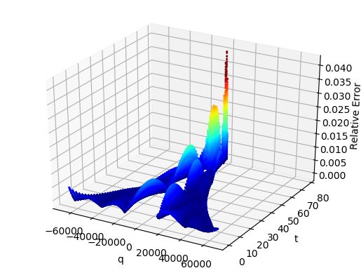
1.   Introduction

Financial mathematics are using stochastic control to ensure that market participants are operating
as intermediaries and not as unilateral risk takers: investment banks have to design risk replicating
strategies, systemic banks have to ensure they have plans in case of fire sales triggered by economic
uncertainty, asset managers have to balance risk and returns in their portfolios and brokers have
to be sure investors’ large buy or sale orders are executed without distorting the prices. The latter
took a primary role in post-2008 markets since participants understood preservation of liquidity is
of primary importance.
   Our paper addresses this last case, belonging to the academic field of optimal trading, initially
introduced by (Almgren and Chriss 2001) and (Bertsimas and Lo 1998), and then extended in a
lot of ways, from sophisticated stochastic control (Bouchard et al. 2011) to Gaussian-quadratic ap-
proximations allowing to obtain closed-form solutions like (Cartea and Jaimungal 2016) or (Cartea
et al. 2015), or under a self-financing equation context, as in (Carmona and Webster 2019). Learn-
ing was introduced in this field either via on-line stochastic approximation (Laruelle et al. 2013) or
in the context of games with partial information (Cardaliaguet and Lehalle 2018). More recently,
Reinforcement Learning (RL) approaches have been proposed, like in (Guéant and Manziuk 2019)
to face the high dimensionality of optimal trading of portfolios, or in (Mounjid and Lehalle 2019)
to adapt the controls in an online way; see also (Charpentier et al. 2020) for an overview.
   For optimal control problems in continuous time, the traditional approach starts with the cost
function and derives, through dynamic programming, a Hamilton-Jacobi-Bellman (HJB) equation
involving the optimal control and the value function (that is the optimum of the Q-function in
RL). This Partial Differential Equation (PDE) can be explicitly written only once the dynamics
to be controlled are stylized enough. When it does not have a closed form solution, this PDE can
be solved either by a deterministic method (like a finite difference scheme) that is limited by the
dimension of the problem, or by RL approaches, like in (Buehler et al. 2019) for deep hedging
or in (Guéant et al. 2020, Tian et al. 2019) for optimal trading. In contrast with (Tian et al.
2019) mentioned above, we focus less on the use of signals in algorithmic trading and more on the
risk control dimension, going into neural network explainability aspects that, to the best of our
knowledge, have not been explored before.
   In the broader literature, deep learning techniques for PDEs and Backward Stochastic Differential
Equations (BSDEs) have recently attracted a lot of interest (Sirignano and Spiliopoulos 2018, Huré
et al. 2019, Raissi et al. 2019, E et al. 2017, Han et al. 2018) and found numerous applications such
as price formation (Sirignano and Cont 2019), option pricing (Liu et al. 2019) or financial systems
with a continuum of agents (Fouque and Zhang 2019, Carmona and Laurière 2019a,b).
   In this paper, we propose to skip most of the previous steps: we directly learn the optimal control
on the discrete version of the dynamics and of the cost function that are usually giving birth to the
HJB, which we no longer have to derive. This approach, also used e.g. in (Gobet and Munos 2005,
Han and E 2016) for optimal control, gives us the freedom to address dynamics for which deriving
explicitly a PDE is not possible, and to learn directly on trajectories coming from real data. In
optimal trading, the control has a feedback loop with the dynamics via price impact: the faster
you trade, the more you move the price in a detrimental way (Bacry et al. 2015). In our setup the
controller sets the trading speed of an algorithm in charge of buying or selling a large amount of
stock shares, solving the trade-off between trading fast to get rid of the exposure to uncertainty of
future prices and trading slow to not pay too much in market impact.
   For numerical applications we use high frequency (HF) data from the Toronto Exchange (TSX)
on 19 stocks over two years, each of them generating around 6,500 trades (i.e. data points) per day.
We compare different controls: controls generated by a widely known stylized version of the problem
that has a closed form formula (Cartea et al. 2015), controls learned on simulated dynamics whose
parameters are estimated on the data in different ways (with or without stationary assumptions),
and controls learned on real data. For the latter case, we transfer the learning from simulated data
to real data, to make sure we start with a good initialization of the controller.
In our setup, a controller maps the state space describing price dynamics and the trader’s in-
ventory to a trading speed that leads to an updated version of the state, and so on until the end
of the trading day. The same controller is used at every decision step, which corresponds to one
decision every 5 minutes. When the controller is a neural net, it is used multiple times before the
loss function can be computed and improved via back propagation, in the spirit of (Lehalle and
Azencott 1998).
  Our first main contribution is that we not only train a neural net for given values of the end-
user’s preferences, but we also train a neural net having two more inputs that are the trader’s
preferences (i.e. risk aversion parameters), so that this neural net is learning the mapping between
the preferences (i.e. hyper-parameters of the control setup) and the optimal controls. To the best of
our knowledge, it is the first time that a neural net is performing this kind of “functional learning”
of risk aversion parameters: the neural net learns the optimal control for a range of cost functions
that are parametrized by the risk preferences. In the paper we call it a “multi-preferences neural
net”.
  The second major contribution of this paper is the way we compare the generated controls in a
meaningful way through model distillation. Model distillation and, more precisely, model translation
methods seek to replicate the DNN behavior across an entire dataset (see Tree-based Frosst and
Hinton (2017), Tan et al. (2018), Zhang et al. (2019), Graph-based Zhang et al. (2016, 2017) and
Rule-based Murdoch and Szlam (2017), Harradon et al. (2018) methods). Our paper introduces a
model translation method focused on the idea of global approximation (see Tan et al. (2018) for a
discussion on global additive explanations).
  Our global distillation approach paves the way to methods which satisfy the request of financial
regulators about the explainability of learned controls. We start by the functional space of controls
spanned by the closed-form solution of the stylized problem: they are non-linear in the remaining
time to trade and affine in the remaining quantity to trade (see (Cardaliaguet and Lehalle 2018)
for a description of the relationship between the optimal controls and the space generated by the
h1 (t) and h2 (t) defined later in the paper). Hence, we project the learned controls on an affine basis
of functions, for each slice of remaining time to trade T − t. In doing so, we provide evidence of
the distance between the black-box controls learned by a neural network, and the baseline control
used by banks and regulators. We can compare the controls in this functional space and, thanks
to the R2 of the linear regressions, we know the average distance between this very transparent
representation of the controls and the ones generated by the neural controllers. In practice, we show
that when the loss function is mainly quadratic, the learned controls, even when they are trained
on real data, are spanning roughly the same functional space as the closed-form ones. End-users
and regulators can consider them with the same monitoring tools and analytics than more standard
(but sub-optimal) controls. When the loss function is more realistic but not quadratic anymore,
taking into account the mean reverting nature of intra-day price dynamics (Labadie and Lehalle
2014), the generated controls may or may not belong to the same functional space.
  The structure of the paper is as follows: Section 2 presents the optimal execution problem setup,
focusing on the loss function and on the closed-form formula associated with the state-of-the-art
optimal execution problem. It also introduces the architecture of the neural networks we use and
our learning strategies. Section 3 describes the dataset, stylized facts of intra-day price dynamics
that should be taken into account, and motivates learning in a data-driven environment. Section 3
also presents the numerical results and our way to tackle explainability of the generated controls.
Conclusions and perspectives are provided in Section 4.
2.     The optimal execution model

2.1.    Dynamics and payoff
Optimal trading is dealing with an agent who would like to execute a large buy or sell order in the
market before a time horizon T . Here, their control is a trading speed νt ∈ R. The center of the
problem is to find the balance between trading too fast (and hence move the price a detrimental
way and pay trading costs, as modelled here in (1) and (3)) and trading too slow (and being
exposed to not finishing the order and be exposed to uncertainty of future prices, reflected in (2)
and (4)). They maximize their wealth while taking into account a running cost and a final cost of
holding inventory, and they are constrained by the dynamics of the system, which is described by
the evolution of the price St , their inventory Qt (corresponding to a number of stocks), and their
wealth Xt (corresponding to a cash amount). In the market, the price process for the asset they
want to trade evolves according to
                                                               √
                                ∆St := St+1 − St = αt νt ∆t + σ ∆t t ,                               (1)

for t = 0, . . . , T − 1, where αt > 0 is a parameter that accounts for the drift, ∆t is the size of a
time step, σ > 0 is a constant volatility term, taken to be the historical volatility of the stock being
traded. For transfer learning on historical data, the database contains real price increments and
hence the realized volatility is (implicitly) of the same order of magnitude.  ∼ N (0, 1) is a noise
term.
   The state of the investor at time t is described by the tuple (T − t, Qt , Xt ). Qt is their inventory,
or number of stocks, and Xt is their wealth at time t, taken as a cash amount. To isolate the
inventory execution problem from other portfolio considerations, the wealth of the agent at time
0 is considered to be 0, i.e. X0 = 0. Suppose the agent is buying inventory (the selling problem
is symmetric). Then, Q0 < 0 and the trading speed ν will be mostly positive throughout the
trajectory. The evolution of the inventory is given by:

                          ∆Qt := Qt+1 − Qt = νt ∆t, for t = 0, . . . , T − 1.                         (2)

The wealth of the investor evolves according to

                               ∆Xt := Xt+1 − Xt = −νt (St + κ · νt )∆t,                               (3)

for t = 0, . . . , T − 1, where κ > 0 is a constant, and the term κ · νt represents the temporary market
impact from trading at time t. As we can see, this is a linear function of νt that acts as an increment
to the mid-price St . It can also be seen as the cost of “crossing the spread”, or a transaction cost.
  The cost function of the investor fits the framework considered e.g. in (Cartea et al. 2015). The
agent seeks to maximize over the trading strategy ν the reward function given by:

                                      h                        T
                                                               X       i
                                                          γ
                         JA,φ (ν) := E XT + QT ST − A|QT | − φ   |Qt |γ ,                             (4)
                                                                     t=0

with γ > 0. We mostly focus on the standard case γ = 2, but we will also consider the case where
γ = 3/2, which better takes into account the sub-diffusive nature of intra-day price dynamics, see
(Labadie and Lehalle 2014). XT , ST , and QT are the random variables parameterizing the terminal
value of the stochastic processes described in the dynamics (1)–(3). A > 0 and φ > 0 are constants
representing the risk aversion of the agent. A penalizes holding inventory at the end of the time
period, and φ penalizes holding inventory throughout the trading day. Together, they parametrize
the control of the optimal execution model and stand for the agent’s preferences.
The trading agent wants to find the optimal control ν for the cost (4) subject to the dynamics
(1)–(3). In the sequel, we solve this problem using a neural network approximation for the optimal
control. As a benchmark for comparison, we will use state-of-the-art closed-form solution for the
corresponding continuous time problem, which is derived through a PDE approach. The closed-
form solution of the PDE is well-defined only when the data satisfies suitable assumptions. The
neural net learns the control νt directly from the data, while finding a closed-form solution for the
PDE is not always possible.
It can be shown, see (Cartea and Jaimungal 2016), that the optimal control ν ∗ is obtained as a
linear function of the inventory, which can be written explicitly as:
h1 (t) α + h2 (t)
ν ∗ (t, q) = + q, (5)
2κ 2κ
where h2 and h1 are the solutions of a system of Ordinary Differential Equations (ODEs).
2.2. Non-parametric solution
The neural network setup. The neural network implementation we propose precludes all the
usual derivations in the (Cartea and Jaimungal 2016) framework. We no longer need to find the PDE
corresponding to the stochastic optimal control problem, we no longer need to break it down into
ODEs and solve the ODE system, and we can try to directly approximate the optimal control. The
deep neural network approximation looks for a control minimizing the agent’s objective function
(4) while being constrained by the dynamics (1)–(3), without any further derivations.
We define one single neural network fθ (·) to be trained for all the time steps. Each iteration of the
stochastic gradient descent (SGD) proceeds as follows. Starting from an initial point (S0 , X0 , Q0 ),
we simulate a trajectory using the control νt = fθ (t, Qt ). Based on this trajectory, we compute
the gradient of associated cost with respect to the neural network’s parameters θ. Finally, the
network’s parameters are updated based on this gradient. In our implementation, the learning rate
is updated using Adaptive Moment Estimation (Adam) (Kingma and Ba 2014), which is well suited
for situations with a large amount of data, and also for non-stationary, noisy problems like the one
under consideration.
In the Monte-Carlo
√ simulation mode, we generate random increments of the Brownian motion
through the term σ ∆t , where ∼ N (0, 1) comes from the standard Gaussian distribution. Using
the Gaussian increments, along with the νt obtained from the neural network, and the three process
updates (∆St , ∆Xt , ∆Qt ), we can compute the new state variables in discrete time:
√
St+1 = St + αt fθ (t, Qt )∆t + σ ∆t , (6)
Xt+1 = Xt − fθ (t, Qt )(St + κt fθ (t, Qt ))∆t, (7)
Qt+1 = Qt + fθ (t, Qt )∆t. (8)
The new state variable Qt+1 , along with the time variable, is then going to serve as input to help us
learn the control at the next time step. This cycle continues until we have reached the time horizon
T . Since we are using the same neural network fθ for all the time steps, we expect it to learn
according to both time and inventory. Note that each SGD iteration requires T steps because we
need the neural net to have controlled the T steps before being able to compute the value function
for the full trajectory. It then backpropagates the error on the terminal value function across the
weights of the same neural net we use at each of the T iterations.
Neural network architecture and parameters. The architecture consists of three dense hidden
layers containing five nodes each, using the hyperbolic tangent as activation function. Each hidden
layer has a dropout rate of 0.2. We add one last layer, without activation function, that returns theoutput. The learning rate is η = 5e−4 ; the mini-batch size is 64; the tile1 size is 3; and the number
of SDG iterations is 100,000. Every 100 SGD iterations, we perform a validation step in order to
check the generalization error, instead of evaluating just the mini-batch error. We used Tensorflow
in our implementation.
Although the neural network’s basic architecture is not very deep, each SGD step involves T
loops over the same neural network. This is because of the closed loop which the problem entails.
The number of layers is thus artificially multiplied by the number of time steps considered.
For the inputs, we have two setups. In the basic setup (as discussed above), the input is the
pair (t, Qt ). In the second case, which we call ”multi-preferences neural network ”, the input is
the tuple (t, Qt , A, φ) and the neural netowrk learns to minimize the JA,φ (·) cost functions for all
(A, φ). Each time we need to solve a given system, we set A and φ to the desired value in the
multi-preferences network and we do not need to relearn anything to obtain the optimal controls.
For both neural nets, the output is the speed of trade νt for each time step t, intercalating with
the variable updates, thus learning a controller for the full length of the trading day.
In order to learn from historical data, we first train the network on data simulated by Monte
Carlo and then perform transfer learning on real data.
2.3. Explainability of the learned controls using projection on a well-known
manifold
We would like to compare the control obtained using the PDE solution with the control obtained
using the neural network approximation. As stated in equation (5), the optimal control can be
written as an affine function of the inventory qt at any point in time, for t ∈ [0, T ]. The shape
of this closed-form optimal control belongs to the manifold of functions of t and q spanned by
[0, T ] × R 3 (t, q) 7→ h1 (t)/(2κ) + (α + h2 (t))/(2κ) · q ∈ R, where the hi (t) are non-linear smooth
functions of t. To provide explainability of our neural controller we project its effective controls
on this manifold. We obtain two non-linear functions h̃1 (t) an h̃2 (t) and a R2 (t) measuring the
distance between the effective control and the projected one at each time step t.
Procedure of projection on the ”closed-form manifold”. For each t, we form a database of
all the learned controls νt mapped by the neural net to the remaining quantity qt . It enables us
to project this νt on qt using an Ordinary Least Squares (OLS) regression whose loss function is
given by:
L(β1 (t), β2 (t)) = ||ν(q(t)) − (β1 (t) + β2 (t)q(t))||22 , (9)
and do a global translation of our neural network control.
The coefficients β1 (t) and β2 (t) of this regression νt = β1 (t) + β2 (t)qt + εt can be easily inverted
to give
h̃1 (t) := 2κ β1 (t), h̃2 (t) := 2κ β2 (t) − α (10)
for each t ∈ [0, T ]. The R2 (t) of each projection associated to t quantifies the distance between the
effective neural ”black box” control and the explained one ν̃t := h̃1 (t)/(2κ) + (α + h̃2 (t))/(2κ) · qt .
The curve of R2 (t) represents how much of the non-linear functional can be projected onto the
manifold of closed-form controls at each t. In practice we perform T = 77 OLS projections to obtain
the curves of h1 , h2 and R2 (see Figure 2) which provide explainability of our learned controls.
1 The tile size (ts) stands for how many samples of the inventory we combine with each sampled pair. For ts = 3, each pair
j
(S0 , {∆Wt }T T
t=0 ) becomes three samples: (Q0 , S0 , {∆Wt }t=0 ), for j ∈ {1, 2, 3}, where j is the tile index. This is useful when
using real data, because we can generate more scenarios than we would ordinarily be able to.Table 1. Descriptive statistics of the TSX stocks used.
Average # Trades per Day: 124,988.4
Average # Trades per Stock: 3,308,902.2
avg. bin spread 1
Permanent Market Impact α: 0.16 · avg. bin volume
· dt
avg. bin spread 1
Temporary Market Impact κ: 0.24 · avg. bin volume
· dt
% of 5-min Bins w/ Data: 91.5%
Users’ preferences and exploration-exploitation issues. The rate at which the agent exe-
cutes the whole inventory strongly depends on the agent’s preferences A and φ. When they are
both large, the optimal control tends to finish to trade earlier than T , the end of the trading day.
Because of that, the trajectories of Qt approach zero in just a few time steps and after that large
values of Qt are not visited during the training phase. As a consequence, in such a regime, it will be
very difficult for the neural net to learn anything around the end of the time interval since it will no
longer explore its interactions with price dynamics to be able to emulate a better control. For the
case of the multi-preferences controller with 4 inputs, including A and φ, taking (A, φ) in a certain
range ensures that the neural net will witness long enough trajectories to exploit them. To this
end, we took profit of the closed-form solution of the stylized dynamics and scanned the duration
of trajectories for each pair (A, φ). In order to avoid the exploration - exploitation trade-off, we
restricted the domain to values of φ smaller or equal to 0.007, and values of A smaller or equal to
0.01. This enabled the regression to learn the functional produced by the neural network. There
will be some inventory left to execute at the end of the trading day for these parameters. For the
pair (A, φ) = (0.01, 0.007), we have less than 1% of the initial inventory left to execute, yet it is
enough for us to estimate the regression accurately.
3. Optimal execution with data
3.1. Data description
We use ticker data for trades and quotes for equities traded on the Toronto Stock Exchange for the
period that ranges from Jan/2008 until Dec/2009, which results in 503 trading days. Both trades
and quotes are available for Level I (no Level II available) for 19 stocks. They have a diverse range
of industries, and daily traded volume. Our method can be directly used for all the stocks, either
individually or simultaneously.1 Table 1 summarizes the database information:
We partition both trade and quote files into smaller pickled files organized by date. We merge
them day by day to calculate other interesting variables, such as: trade sign, volume weighted
average price (VWAP), and the bid-ask spread at time of trade. We drop odd-lots from the dataset,
as they in fact belong to a separate order book. Moreover, we only keep the quotes that precede a
trade, or a sequence of trades. It saves us memory usage and processing times.
The trade data, including the trade sign variable, is further processed into five minute bins. We
have picked five minute intervals because, while the interval could be changed, here we want to
make sure the data is not too sparse, and to provide additional risk control to the agent over a
time horizon of one full day. TAQ data is extremely asynchronous and a situation might happen
when there is not enough data in a given time interval. To avoid this problem, we aggregate the
data into bins and focus our analysis on liquid stocks. This bin size is big enough for us to have
data at each bin, and small enough to allow the agent to adjust the trading speed several times
throughout the day. Since the market is open from 9:30 until 16:00, five-minute bin intervals, we
1 Forthe market impact parameters (α, κ), we estimate the same value for all the stocks through a normalization, then we
de-normalize the parameters using the seasonality profile of the stock used in the model.Figure 1. QQ-plot (top left), auto-correlation function (top-right), intra-day seasonalities (bottom) of price dynamics have 78 time steps, which gives us 77 bins for which to estimate the control on each trading day. We have 91.5% of bins containing data (see Table 1). 3.2. Important aspects of financial data The stylized dynamics allowing a PDE formulation of the problem and a closed-form solution of the control make a lot of assumptions on the randomness of price increments, market impact and trad- ing costs. Typically they assume independent and normally distributed, stationary, non-correlated returns, with no seasonality. However, these properties typically do not hold true for financial time series. See (Bouchaud et al. 2018, Campbell et al. 1993) for some interesting discussions. Figure 1 shows the specific characteristics of financial data for the stock MRU. The left plot is a qq-plot, which tells us that the stock returns have a heavy tailed distribution. The same is confirmed for all stocks: we observe high kurtosis (ranging from 163 to 11302) for all the distributions of stock returns (which is a common metric for saying that a distribution has heavy tails with respect to a Gaussian distribution). The middle plot presents the five-minute lag auto-correlation profile. For this stock, we can see a mean-reversion tendency for five minutes and one hour. The first lag of the five-minute auto-correlation (ranging from −0.017 to −0.118) indicates all stocks present this feature. The right plot shows intra-day seasonality profiles: the bid-ask spread (blue, dashed curve), and the intra-day volume curve (full, gray curve). As mentioned in section 2.3, the first step is to compare the output of our neural network model to the PDE solution, both using Monte Carlo simulated data. The second step is to understand how seasonality in the data might affect the training and the output. Finally, we continue our learning process on real data, in order to learn its peculiarities in terms of heavy tails, seasonality and auto-correlation.
h1                                                                   h2
                                                                                0.000
   300
                                                                                0.002
   200
   100                                                                          0.004
       0                                                                        0.006
   100                  Stylized closed-form
                        NNet on simulations                                     0.008
   200
                        NNet on simulations with seasonality
   300                  NNet on real data with seasonality                      0.010
                        Multi-preference NNet on real data with seasonality
           0       10       20     30      40      50      60      70     80            0   10    20     30     40   50    60   70   80
                                         Time                                                                 Time
                                           R2                                                    Average Control Process (nu)
 1.0000                                                                        90000
 0.9995                                                                        80000

 0.9990                                                                        70000
                                                                               60000
 0.9985
                                                                               50000
 0.9980
                                                                               40000
 0.9975                                                                        30000
 0.9970                                                                        20000
               0   10        20     30      40      50     60      70     80            0   10    20    30      40   50    60   70   80
                                          Time                                                                Time

Figure 2. Explainable parts of the control: h1 (t), h2 (t); fraction of the explained control R2 (t), and average control
given it is positive E(ν(t)|ν(t) > 0) for different controllers.

3.3.       PDE vs DNNs: from Monte Carlo to real data
The results and our benchmark are summarized in Figure 2. As stated in equation (5), the optimal
control for the stylized dynamics and the PDE is linear in the inventory, hence the associated R2
is obviously 1 for any t. For the different neural nets, we perform the projections on the (h1 , h2 )
manifold and keep track of the R2 curve.
   During the learning, it is important that the neural network can observe full trajectories. When
the risk aversion parameters are very restrictive, the closed-form solution and neural net trades so
fast that the order is fully executed (i.e. the control stops) far before t = T . Because of that it
is impossible to learn after this stopping time corresponding to qt = 0. Our workaround for this
exploration - exploitation issue has been to use the closed-form solution to select a range of (A, φ)
allowing the neural net to generate enough trajectories to observe the dynamics up to t = T . In
Figure 2, we use the pair (A, φ) = (0.01, 0.007) with γ = 2. We stress that, once the model has
been trained on a variety of pairs (A, φ), we can then use it with new pairs of parameters.
   In this Figure 2, we mix closed-form controls on the stylized dynamics, neural controls on the
same dynamics (using Monte Carlo simulations), neural controls in more realistic simulations (with
an intra-day seasonality) and ultimately on real data. In particular, we use stock data (via transfer
learning, see the thick purple and solid pink lines), and in order to make the model as close as
possible to reality in a version that is in-between synthetic data and transfer learning (dotted pink
curve). We include intra-day seasonality for both volume and bid-ask spread, and we emphasize
how it is reflected in the learned control. We also superpose results for neural networks trained
only on this regime of preferences and the controls of the multi-preference neural network, that is
trained only once and then generates controls for any pair (A, φ) of preferences. The top panels
represent the two components of the projection of the control on the ”closed-form manifold”, to
enable comparison. The plot on the upper left of Figure 2 corresponds to the h1 component. The y-axis scale is in the order of the median of the inventory path, to allow for a fair comparison to h2 · Q. It is naturally very close to zero, since there is no mean-field component in the market impact term. The upper right plot corresponds to the h2 component. We notice that the stylized closed-form and the neural network simulation using Monte Carlo generated paths match perfectly, thus setting a great benchmark for the neural network. The improvements we add to the neural network model, simulations including seasonality, real data with seasonality and multi-preferences all overlap, indicating that the intra-day seasonality component is the most relevant when explain- ing differences in optimal execution speed when departing from the closed-form stylized model. The R2 (t) curves (bottom-left panel) are flat at 1 for the closed form formula (since 100% of the control belongs to this manifold), whereas it can vary for the other controls (see Figure 3, and discussion in section 3.4). Thanks to this projection, it is straightforward to compare the behaviour of all the controls. The R2 (t) curves provide evidence that in this regime the neural controls are almost 100% explained by the closed-form manifold (notice that the y-axis has a very tight range close to 1). It does not say that they are similar to the closed-form solutions of the stylized problem, but that they are linear in qt (but not in t) for each time step t ∈ [0, T ]. Saving the best for last, we present the optimal control for each different configuration in the bottom left plot of Figure 2. We again stress the similarity between the neural network model on simulations versus the closed-form benchmark. We further observe the differences between the opti- mal controls for the improved setups. When we start taking into account the intra-day seasonality, the execution speed adjusts according to the volume traded and to the bid ask spread. It results in less trading when the spreads are large, and in more trading when there is more volumes. In adjusting to market conditions, we are able to improve on the existing execution benchmark. Main differences between the learned controls. Going from stylized dynamics to simulations with intra-day seasonality, and then to real price dynamics does not significantly change the mul- tiplicative term of qt , but it does shift the trading speed. This has been already observed in the context of game theoretical frameworks (Cardaliaguet and Lehalle 2018). When the seasonality is added in the simulation (thick purple curve) the deformation of the control exhibits oscillations that most probably stem from the seasonalities of the bottom panel of Figure 1. The shift learned on real price dynamics (solid pink) amplifies some oscillations that are now less smooth; this is probably due to autocorrelations of price innovations. Moreover Figure 2 shows that the ”func- tional learning” worked: the mono-preference neural network trained only on this (A, φ) and the multi-preferences one have similar curves. 3.4. Nonlinear aspect of DNN controllers For non quadratic costs (we took γ = 3/2 since it is a realistic case, see Labadie and Lehalle (2014)) we take (A, φ) = (0.5, 0.1) to be in a comparable regime as the controls in Figure 2, and (A, φ) = (0.01, 0.007) which results in a non-linear control. The solid blue R2 (t) curve in the bottom left of Figure 3 being again close to one shows that for this combination of parameters, the learned control remains extremely similar to the closed-form manifold. This kind of evidence can allow risk departments of banks and regulators to get more comfortable with this learned control and it can give guidelines to large institutional investors, such as pension funds, to execute their orders in the market with the view of controlling risk in an explicit fashion. When γ = 3/2, the chosen set of risk parameters has more influence in the learned control, which can now either be linear or non-linear. For the pair (A, φ) = (0.01, 0.007), the absolute value of “proportional term” h2 is very close to zero when using the same scale as the h2 when (A, φ) = (0.5, 0.1). Nevertheless, it is compensated by the part of the control that is outside of this space, as indicated by the R2 : at the start of the trading process 40% of the control is explained by the “closed-form manifold”; it then decreases to 0%, meaning that the learned control takes part fully out of this manifold; but it then increases back to 80% at the end of the
h1                                                                          h2
                                                                                         0.0000
   10000
                                                                                         0.0025
       5000                                                                              0.0050
                                                                                         0.0075
         0
                                                                                         0.0100
       5000                                                                              0.0125

                                                               (A, ) = (0.5, 0.1)        0.0150
   10000                                                       (A, ) = (0.01, 0.007)     0.0175
              0        10        20        30      40     50       60      70      80                 0    10     20    30     40    50   60   70   80
                                                 Time                                                                        Time
                                                R2                                                              Average Control Process (nu)
  1.0                                                                                   80000
                                                                                        70000
  0.8                                                                                   60000
                                                                                        50000
  0.6
                                                                                        40000
  0.4                                                                                   30000
                                                                                        20000
  0.2                                                                                   10000
                                                                                            0
  0.0
          0       10        20        30          40     50       60       70      80             0       10     20    30      40   50    60   70   80
                                                Time                                                                         Time

                                                        Figure 3. h1 , h2 , R2 , ν: for the case γ = 3/2

process. It seems that the best way to finish the trading is already well captured by the closed-form
manifold. As we observe from the control plot in the bottom-right of Figure 3, the parameter pair
(A, φ) = (0.01, 0.007) does not enforce trading speeds as fast as the pair (A, φ) = (0.5, 0.1) when the
loss function is sub-diffusive. Keeping the same preferences as before is thus making the trader less
aggressive in a sub-diffusive environment. In order to have the same behavior in terms of control,
they would need to behave in a more risk averse manner.

3.5.      Comparison to State-of-the-Art
In Figure 4, we compare the performance of the control learnt by the neural network with state-of-
the-art control. For the sake of illustration, we focus here on two cases: γ = 2 and γ = 3/2. Given
q0 and a choice of control, using Monte Carlo samples we compute an approximation of the reward
function (corresponding to (4) conditioned on Q0 = q0 ) and the marked-to-market final wealth in
cash. In the case γ = 2, using the neural network control (with or without seasonality, and also in
the multi-preference setting) almost matches the optimal one obtained by the closed-form solution.
When γ = 3/2, the control stemming from the neural network performs better than the control
coming from the closed-form solution (recall that the goal is to maximize the reward function).
We stress that while the reward function is asymmetric due to the intrinsic asymmetry in equation
(3), the marked-to-market wealth defined by MTMT = sign(Q0 )(Q0 S0 − XT ) is symmetric except
for a sign adjustment.
Value Function vs Q0, = 2 MTM Wealth vs Q0, = 2
1000000 Stylized closed-form
1000000 NNet on simulations
NNet on simulations with seasonality
0 Multi-preference NNet with seasonality
500000
1000000
Value Function
MTM Wealth
0
2000000
3000000 500000
Stylized closed-form
NNet on simulations
4000000 NNet on simulations with seasonality
Multi-preference NNet with seasonality 1000000
0 0 0 0 0 0 000 0 0 0 0 00 00 00
6000 4000 2000 2 000 4000 60 600
0
400
0
200
0
200 400 600
Q0 Q0
Value Function vs Q0, = 3/2 MTM Wealth vs Q0, = 3/2
Stylized closed-form 1500000 Stylized closed-form
1000000 NNet on simulations NNet on simulations
1000000
0
500000
1000000
Value Function
MTM Wealth
0
2000000
3000000 500000
4000000 1000000
5000000 1500000
00 00 00 0 00 00 00 00 00 00 0 00 0 0 00
600 400 200 200 400 600 600 400 200 200 400 600
Q0 Q0
Figure 4. Value Functions (left) and Marked-to-Market Wealth (right): for γ = 2 (top) and γ = 3/2 (bottom)
3.6. Empirical Verification of DNN Explainability
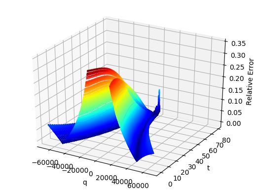
Figure 5 displays the DNN control and relative error in the neural network regression, namely,
if (t, q) 7→ fθ (t, q) and (t, q) 7→ f˜θ (t, q) denote respectively the trained neural network and ap-
proximate version obtained by regression, we compute: (t, q) 7→ |(fθ (t, q) − f˜θ (t, q))/f˜θ (t, q)|. The
maximum relative error for the case γ = 2 is 0.04, while for the case γ = 3/2 it is 0.35. We see
that for most time steps, the relative error is small in the bulk of the distribution of qt . However,
around the terminal time = 78, the distribution is very concentrated around q = 0, which explains
why the regression is less accurate.
4. Conclusion
In this paper, we succeed in using a neural network to learn the mapping between end-user prefer-
ences and the optimal trading speed, allowing to buy or sell a large number of shares or contracts
on financial markets. Prior to this work, various proposals have been made but the learned con-
trols have always been specialized for a given set of preferences. Here, our multi-preferences neural
network learns the solution of a class of dynamical systems.
Note that optimal execution dynamics are reacting to the applied control, via the price impact of
the buying or selling pressure. The neural network hence has to learn this feedback. Our approach
uses a deep neural network, whose inputs are user preferences and the state of the optimization
problem that change after each decision. The loss function can only be computed at the end of
the trading day, once the neural controller has been used 77 times. The backpropagation henceFigure 5. Relative error in the regression: γ = 2 (left) and γ = 3/2 (right) takes place across these 77 steps. We faced some exploration - exploitation issues and solved it by choosing suitable the range of users’ preferences to ensure that long enough trajectories are observed during the learning. Our setup leverages on transfer learning, starting on simulated data before switching to historical data. Since we want to understand how the learned controls are different from the closed-form solution on a stylized model that are largely used by practitioners, we learn on different versions of simulated data: from a model corresponding to the stylized one to one incorporating non- stationarities, and then to real data. To ensure the explainability of our learned controls, we introduce a projection method on the functional space spanned by the closed-form formula. It allows us to show that most of the learned controls belong to this manifold. When we depart from the traditional model by incorporating a risk aversion term, the learned control is close to its projected version on the bulk of the distribution, supporting the idea that the projection explains a significant part of the neural network control. Furthermore, the source of adaptation to realistic dynamics focuses on a ”shift term” h1 in the control. The most noticeable adaptation of h1 exhibits slow oscillations that are most probably reflecting the seasonalities of intra-day price dynamics. We then introduce a version of the loss function that reflects more the reality of intra-day price dynamics (that are sub-diffusive). Despite the fact that the associated HJB has no closed form solution, we manage to learn its associated optimal control and show, using our projection technique, that it almost belongs to the same manifold. This approach delivers explainability of learned controls and can probably be extended to contexts other than optimal trading. It should help regulators to have a high level of trust in the learned controls, that are often considered as “black boxes”: our proposal exposes the fraction of the controls that belongs to the manifold practitioners and regulators are familiar with, allowing them to perform the usual ”stress tests” on it, and quantifies this fraction as a R2 curve that is easy to interpret. More details on the ethical impact and broad societal implications are discussed in Appendix C.
References

Almgren, R. and Chriss, N., Optimal execution of portfolio transactions. Journal of Risk, 2001, 3, 5–40.
Bacry, E., Iuga, A., Lasnier, M. and Lehalle, C.A., Market impacts and the life cycle of investors orders.
     Market Microstructure and Liquidity, 2015, 1, 1550009.
Bertsimas, D. and Lo, A.W., Optimal control of execution costs. Journal of Financial Markets, 1998, 1,
     1–50.
Bouchard, B., Dang, N.M. and Lehalle, C.A., Optimal control of trading algorithms: a general impulse
     control approach. SIAM Journal on financial mathematics, 2011, 2, 404–438.
Bouchaud, J.P., Bonart, J., Donier, J. and Gould, M., Trades, quotes and prices: financial markets under
     the microscope, 2018, Cambridge University Press.
Buehler, H., Gonon, L., Teichmann, J. and Wood, B., Deep hedging. Quantitative Finance, 2019, 19, 1271–
     1291.
Burgess, M., Australia Pension Funds Fear Early Access May Compound Pressure. Bloomberg News, 2020.
Campbell, J.Y., Grossman, S.J. and Wang, J., Trading volume and serial correlation in stock returns. The
     Quarterly Journal of Economics, 1993, 108, 905–939.
Cardaliaguet, P. and Lehalle, C.A., Mean field game of controls and an application to trade crowding.
     Mathematics and Financial Economics, 2018, 12, 335–363.
Carmona, R. and Laurière, M., Convergence Analysis of Machine Learning Algorithms for the Numerical
     Solution of Mean Field Control and Games: I–The Ergodic Case. arXiv preprint arXiv:1907.05980,
     2019a.
Carmona, R. and Laurière, M., Convergence Analysis of Machine Learning Algorithms for the Numerical So-
     lution of Mean Field Control and Games: II–The Finite Horizon Case. arXiv preprint arXiv:1908.01613,
     2019b.
Carmona, R. and Webster, K., The self-financing equation in limit order book markets. Finance and Stochas-
     tics, 2019, 23, 729–759.
Cartea, Á. and Jaimungal, S., Incorporating order-flow into optimal execution. Mathematics and Financial
     Economics, 2016, 10, 339–364.
Cartea, Á., Jaimungal, S. and Penalva, J., Algorithmic and high-frequency trading, 2015, Cambridge Uni-
     versity Press.
Charpentier, A., Elie, R. and Remlinger, C., Reinforcement Learning in Economics and Finance. arXiv
     preprint arXiv:2003.10014, 2020.
Dean, J., Corrado, G., Monga, R., Chen, K., Devin, M., Mao, M., Ranzato, M., Senior, A., Tucker, P., Yang,
     K. et al., Large scale distributed deep networks. In Proceedings of the Advances in neural information
     processing systems, pp. 1223–1231, 2012.
E, W., Han, J. and Jentzen, A., Deep learning-based numerical methods for high-dimensional parabolic
     partial differential equations and backward stochastic differential equations. Communications in Math-
     ematics and Statistics, 2017, 5, 349–380.
Fouque, J.P. and Zhang, Z., Deep Learning Methods for Mean Field Control Problems with Delay. arXiv
     preprint arXiv:1905.00358, 2019.
Frosst, N. and Hinton, G., Distilling a neural network into a soft decision tree. arXiv preprint
     arXiv:1711.09784, 2017.
Gobet, E. and Munos, R., Sensitivity analysis using Itô-Malliavin calculus and martingales, and application
     to stochastic optimal control. SIAM J. Control Optim., 2005, 43, 1676–1713.
Guéant, O. and Manziuk, I., Deep reinforcement learning for market making in corporate bonds: beating
     the curse of dimensionality. arXiv preprint arXiv:1910.13205, 2019.
Guéant, O., Manziuk, I. and Pu, J., Accelerated share repurchase and other buyback programs: what neural
     networks can bring. Quantitative Finance, 2020, pp. 1–16.
Han, J. and E, W., Deep learning approximation for stochastic control problems. Deep Reinforcement Learn-
     ing Workshop NIPS, 2016.
Han, J., Jentzen, A. and E, W., Solving high-dimensional partial differential equations using deep learning.
     Proceedings of the National Academy of Sciences, 2018, 115, 8505–8510.
Harradon, M., Druce, J. and Ruttenberg, B., Causal learning and explanation of deep neural networks via
     autoencoded activations. arXiv preprint arXiv:1802.00541, 2018.
Huré, C., Pham, H. and Warin, X., Some machine learning schemes for high-dimensional nonlinear PDEs.
     arXiv preprint arXiv:1902.01599, 2019.
Keskar, N.S., Mudigere, D., Nocedal, J., Smelyanskiy, M. and Tang, P.T.P., On large-batch training for deep
learning: Generalization gap and sharp minima. arXiv preprint arXiv:1609.04836, 2016.
Kingma, D.P. and Ba, J., Adam: A method for stochastic optimization. arXiv preprint arXiv:1412.6980,
2014.
Labadie, M. and Lehalle, C.A., Optimal starting times, stopping times and risk measures for algorithmic
trading. The Journal of Investment Strategies, 2014, 3.
Laruelle, S. and Lehalle, C.A., Market microstructure in practice, 2018, World Scientific.
Laruelle, S., Lehalle, C.A. and Pagès, G., Optimal posting price of limit orders: learning by trading. Math-
ematics and Financial Economics, 2013, 7, 359–403.
Lehalle, C.A. and Azencott, R., Piecewise affine neural networks and nonlinear control. In Proceedings of
the International Conference on Artificial Neural Networks, pp. 633–638, 1998.
Liu, S., Oosterlee, C.W. and Bohte, S.M., Pricing options and computing implied volatilities using neural
networks. Risks, 2019, 7, 16.
Masters, D. and Luschi, C., Revisiting small batch training for deep neural networks. arXiv preprint
arXiv:1804.07612, 2018.
Mounjid, O. and Lehalle, C.A., Improving reinforcement learning algorithms: towards optimal learning rate
policies. arXiv preprint arXiv:1911.02319, 2019.
Murdoch, W.J. and Szlam, A., Automatic rule extraction from long short term memory networks. arXiv
preprint arXiv:1702.02540, 2017.
Patzelt, F. and Bouchaud, J.P., Universal scaling and nonlinearity of aggregate price impact in financial
markets. Physical Review E, 2018, 97, 012304.
Raissi, M., Perdikaris, P. and Karniadakis, G.E., Physics-informed neural networks: A deep learning frame-
work for solving forward and inverse problems involving nonlinear partial differential equations. Journal
of Computational Physics, 2019, 378, 686–707.
Sirignano, J. and Cont, R., Universal features of price formation in financial markets: perspectives from deep
learning. Quantitative Finance, 2019, 19, 1449–1459.
Sirignano, J. and Spiliopoulos, K., DGM: a deep learning algorithm for solving partial differential equations.
J. Comput. Phys., 2018, 375, 1339–1364.
Tan, S., Caruana, R., Hooker, G., Koch, P. and Gordo, A., Learning global additive explanations for neural
nets using model distillation. arXiv preprint arXiv:1801.08640, 2018.
Tian, C., Tao, S., Maarek, P. and Zheng, L., Learning to Trade with Market Signals. Neurips Workshop on
Robust AI in Financial Services, 2019.
Wilson, D.R. and Martinez, T.R., The general inefficiency of batch training for gradient descent learning.
Neural networks, 2003, 16, 1429–1451.
Zhang, Q., Cao, R., Shi, F., Wu, Y.N. and Zhu, S.C., Interpreting cnn knowledge via an explanatory graph.
arXiv preprint arXiv:1708.01785, 2017.
Zhang, Q., Cao, R., Wu, Y.N. and Zhu, S.C., Growing interpretable part graphs on convnets via multi-shot
learning. arXiv preprint arXiv:1611.04246, 2016.
Zhang, Q., Yang, Y., Ma, H. and Wu, Y.N., Interpreting cnns via decision trees. In Proceedings of the
Proceedings of the IEEE Conference on Computer Vision and Pattern Recognition, pp. 6261–6270,
2019.Appendix A: Details on Explicit Solution and Implementation
A.1. Details on the explicit solution
For the sake of completeness, we recall how the benchmark solution is obtained; see (Cartea and
Jaimungal 2016) for more details. The continuous form of the problem defined in equations (1) to
(4) of the paper, when γ = 2, can be characterized by the value (we drop the subscripts A and φ
to alleviate the notations)
EX0 ,S0 ,Q0 [V (0, X0 , S0 , Q0 )],
where V is the value function, defined as:
h Z T i
2
V (t0 ,x, s, q) = sup E XT + QT ST − A|QT | − φ |Qt |2
ν t0
dSt = α(µt + νt )dt + σdWt
dQt = νt dt
(A1)
subject to dXt = −νt (St + κνt )dt
St > 0, ∀t
X = x, Q = q, S = s.
t0 t0 t0
From dynamic programming, we obtain that the value function V satisfies the following Hamilton-
Jacobi-Bellman (HJB): for t ∈ [0, T ), x, s, q ∈ R,
1
∂t V − φq 2 + σ 2 ∂S2 V + αµ∂S V
2
n o
+ sup αν∂S V + ν∂q V − ν(s + κν)∂X V = 0 (A2)
ν
with terminal condition V (T, x, s, q) = x + q(s − Aq).
If we use the ansatz V (t, x, s, q) = x + qs + u(t, q), with u of the form u(t, q) = h0 (t) + h1 (t)q +
2
h2 (t) q2 , the optimal control resulting from solving this problem can be written as:
αq + ∂q u(t, q) h1 (t) α + h2 (t)
ν ∗ (t, q) = = + q. (A3)
2κ 2κ 2κ
Hence, h1 (t) and h2 (t) act over the control by influencing either the intercept of an affine function
of the inventory, in the case of h1 (t), or its slope, in the case of h2 (t).
From the HJB equation, these coefficients are characterized by the following system of ordinary
differential equations (ODEs):
˙ 1 2
α 1 2
h2 (t) = 2φ − 2κ α − κ h2 (t) − 2κ h2 (t),
h˙1 (t) + 2κ
1
(α + h2 (t))h1 (t) = −αµ(t), (A4)
˙
1 2
h0 (t) = − 4κ h1 (t)
with terminal conditions:
h0 (T ) = 0,
h1 (T ) = 0, (A5)
h2 (T ) = −2A.
Qti+1

                                       ti                  κt

                                                   νt            Xti+1

                                       Qti                αt

                                                                 Sti+1

                                                          t

                     Figure A1. Structure of the state variables’ simulation - One Step

            t0                   t1                      t2                                T

           Qt0                   Qt0                     Qt2                               QT
                      ν0                      ν1                         ···     νT −1
           Xt0                   Xt0                     Xt2                               XT

           St0                   St0                     St2                               ST

                     Figure A2. Structure of the State Variables’ Simulation - All Steps

A.2.   Details on the implementation
In this section, we provide more details on the implementation of the method based on neural
network approximation. For the neural network, we used a fully connected architecture, with three
hidden layers, five nodes each.
  One forward step in this setup is described by Figure A1, while one round of the SGD is rep-
resented by Figure A2. The same neural network learns from the state variables obtained in the
previous step. It thus learns the influence of its own output through many time steps. We have
experimented with using one neural network per time step. However, this method implies more
memory usage, and did not provide any clear advantage with respect to the one presented here.
  From Figures A1 and A2, we can clearly see the idea that the control influences the dynamics.
We are, in fact, optimizing in a closed-loop learning environment, where the trader’s actions have
both permanent and temporary market impact on the price.
  The mini-batch size we used, namely 64, is relatively small. While papers like (Dean et al. 2012)
defend the use of larger mini-batch sizes to take advantage of parallelism, smaller mini-batch sizes
such as the ones we use are shown to improve accuracy in (Keskar et al. 2016), (Masters and Luschi
2018) and (Wilson and Martinez 2003).
  Simulations are run on a MacOS Mojave laptop with 2.5 GHz Intel Core i7 and 16G of RAM,
without GPU acceleration. Available GPU cluster did not increase the average speed of the simu-
lations. Tests done on CPU clusters composed of Dell 2.4 GHz Skylake nodes also did not indicate
relevant speed improvements.

A.3.   Kurtosis and Auto-correlation of stock returns
Table A1 shows the values of kurtosis and auto-correlation for all the stocks. They respectively
indicate that the returns have heavy tails and are auto-correlated. Neither of these characteristics
of real stock returns are taken into account in the baseline model, but they are easily accounted
for in the deep neural network setup presented in the paper.
Table A1. Kurtosis and auto-correlation of intra-day returns
Kurtosis ABX AEM AGU BB BMO BNS COS
222 264 1825 2344 1796 2087 2528
DOL GIL GWO HSE MRU PPL RCI.B
163 7746 507 2975 319 7006 2188
RY SLF TRI TRP VRX
2648 11302 403 7074 213
Auto-correlation ABX AEM AGU BB BMO BNS COS
(lag = 5 min) -.025 -.026 -.03 -.031 -.026 -.03 -.041
DOL GIL GWO HSE MRU PPL RCI.B
-.118 -.047 -.094 -.02 -.105 -.15 -.062
RY SLF TRI TRP VRX
-.017 -.07 -.04 -.066 -.075Appendix B: Learning the mapping to the optimal control in a closed loop
B.1. Details on market impact parameters estimation
Permanent market impact. Let S be the space of stocks; and D be the space of trading days.
If we take five-minute intervals (indicated by the superscript notation), we can write equation (1)
for each stock s ∈ S, for each day d ∈ D, and for each five-minute bin indexed by t as:
5min
√
∆Ss,d,t = αs,t µ5min 5min
s,d,t ∆t + σs ∆ts,d,t , (B1)
where the subscripts s, d, t respectively indicate the stock, the date, and the five-minute interval to
which the variables refer, and ∆t = 5 min, by construction. We have αs,t independent of d, which
assumes that for any given day the permanent market impact multiplier the agent may have on
the price of a particular stock s, for a given time bin t is the same. And we have σs independent
of the day d and time bin t, which means the volatility related to the noise term is constant for a
given stock.
As an empirical proxy for the theoretical value µ5mins,d,t representing the net order flow of all the
agents, we use the order flow imbalance observed in the data: Imb5min s,d,t . We define this quantity as:
t+5min t+5min
buy
X X
Imb5min
s,d,t = vs,d,j − sell
vs,d,j , (B2)
j=t j=t
buy sell is the volume of a sell trade, and we aggregate
where vs,d,t is the volume of a buy trade, and vs,d,t
their net amounts over five minute bins.
However, since we estimate the permanent market impact parameter α using data from different
stocks, and we would like to perform a single regression for all of them, we re-scale the data used
in the estimation. In order to make the data from different stocks comparable, we do the following:
5min ) by the average bin spread over all days for the
(i) Divide the trade price difference (∆Ss,d,t
given stock, also calculated in its respective five minute bin:
5min
∆Ss,d,t
5min
∆S s,d,t = 1 P 5min
, (B3)
|D| d∈D ψs,d,t
5min is the bid-ask spread for a given (stock, date, bin) tuple.
where ψs,d,t
(ii) Divide the trade imbalance (Imb5min
s,d,t ) by the average bin volume over all days for the given
stock, calculated on the respective five minute bin:
5min Imb5min
s,d,t
Imbs,d,t = . (B4)
1
Volume5min
P
|D| d∈D (Total s,d,t )
where Total Volume5min
s,d,t stands for the total traded volume for both buys and sells for a
given (stock, date, bin) tuple.
This ensures that both the volume and the price are normalized to quantities that can be com-
pared. Each (s, d, t) now gives rise to one data point, and we can thus run the following regression
instead, using comparable variables, to find ᾱ:
5min 5min
∆S s,d,t = ᾱ · Imbs,d,t + ¯5min
s,d,t , (B5)where ᾱ is the new slope parameter we would like to estimate, and ¯5min
s,d,t is the normalized version
of the residual we had in equation (B1).
In order to use ᾱ in a realistic way, we de-normalize the regression equation for each stock by
doing:
!
5min ᾱ ψ̄s,t √
∆Ss,d,t = · Imb5min
s,d,t + σ ∆t5min
s,d,t . (B6)
∆t V̄s,t
where V̄s,t is the average bin volume for stock s at bin the time bin t, ψ̄s,t is the average bin bid-ask
spread for the same pair (s, t).
The derivation for the temporary market impact κ uses equation (2) in the paper, and follows
similar steps.
Temporary market impact. The κ parameter represents the magnitude of the trading cost of
an agent in the market. This is an indirect cost incurred by the trader due to the impact that their
order has in the market mid-price. From the dynamics of the wealth process dXt = −νt (St +κνt )dt,
we are assuming that the trading cost is linear in the speed of trading. Notice that the faster the
agent needs to trade, the larger the cost incurred, and the opposite is true for slower trading. We
can re-normalize (B.1) by rewriting it as:
dXt
δx := (−1) · = St + κνt . (B7)
νdt
Then, for each stock s ∈ S, for each day d ∈ D, and for each five-minute bin indexed by t, we
would like to estimate the following expression:
δx5min 5min 5min 5min
s,d,t = Ss,d,t,start + κνs,d,t + s,d,t . (B8)
where the subscript ‘start’ indicates that we are using the mid-price at the start of the five-minute
bin indexed by t.
Since we do not have access to ν, as it is private information for each trader, we would like to
compensate by restricting our statistical analysis to bins that are dominated by only one trader,
but not so much as to have stagnant prices. With the goal of isolating one trader from the crowd
in mind, we seek to restrict our dataset based on the imbalance and on the size of the dominating
traded volume in a given bin.
We extract the trade volume for each bin as the maximum between the aggregate buy volume
and the aggregate sell volume for that particular bin. With this criteria we simultaneously define
whether we have a buy or a sell, and thus the sign of the trade (+1 for buys, and -1 for sells). In
mathematical terms, the dominant trading volume by bin, Ds,d,t5min , can be expressed as:
nP o
t+5min buy Pt+5min sell
max5min j=t vs,d,j , j=t vs,d,j
5min
Ds,d,t = 1 P 5min
. (B9)
|d| d∈D (vs,d,t )
where all variables have been defined in the paragraph about Permanent market impact.
As Patzelt and Bouchaud (2018) find, aggregate-volume impact saturates for large imbalances,
on all time scales, and highly biased order flows are associated with very small price changes.
They find that the probability for an order to change the price decreases with the local imbalance,
and vanishes when the order signs are locally strongly biased in one direction. However, if we first
5min , the imbalances are naturally
restrict the data to having the dominant trading volume by bin Ds,d,t
restricted. Hence, we do not need to further restrict the upper bound of the imbalance. However,You can also read