Application of Machine Learning techniques in Cloud Services
←
→
Page content transcription
If your browser does not render page correctly, please read the page content below
National and Kapodistrian
          University of Athens
          Department of Physics and Informatics and
          Telecommunications

      Master Thesis in Control and Computing

Application of Machine Learning techniques
             in Cloud Services

                   Antonia Pelekanou
                  Student ID: 2015518

                      Supervisor
           Assistant Professor Anna Tzanakaki

                 Athens, October 2017
Master Thesis in Control and Computing
Title: “Application of Machine Learning techniques in Cloud Services”
Author: Antonia Pelekanou
Student ID: 2015518
Supervisor: Assistant Professor Anna Tzanakaki
Evaluation Committee: Assistant Professor Anna Tzanakaki,
                       Associate Professor Dionysios I. Reisis,
                       Associate Professor Hector E. Nistazakis
Master Thesis submitted October 2017
Key words: Big Data, Cloud, IoT, Machine Learning, Neural Networks, Forecasting

                                    ABSTRACT

This thesis focuses on machine learning techniques that can be used in support of
cloud services. The motivation behind this work is the necessity of manipulation and
processing data comprising multiple sensor measurements. These measurements
were collected by sensors that were installed on the Reims tramway. The concepts of
Big Data are studied, while different Data Mining methods and Machine Learning
algorithms are presented. A review of Cloud Computing, Internet of Things and
SiteWhere are also provided. Two different neural network structures, Multilayer
Perceptrons and Long Short-Term Memory to process and forecast the data composed
of various physical quantities of the Reims tramway are studied. The results produced
indicate that Long Short-Term Memory is more suitable than Multilayer Perceptrons
for this forecasting problem.

                                                                                   2
ACKNOWLEDGEMENTS

         I would like to express my gratitude to Professor Anna Tzanakaki, my thesis
supervisor, for her guidance and encouragement. The door to Prof. Tzanakaki’s office
was always open whenever I had a question about my research or writing. She allowed
this paper to be my own work, while with her useful critiques steered me in the right
direction.

         I would also like to extend my thanks to Dr. Markos Anastasopoulos for his
general advices and his suggestions concerning the way I should approach certain
aspects of this research work.

         Finally, I wish to thank my family for their continuous support throughout the
process of researching and writing this thesis. This accomplishment would not have
been possible without them.

Author

Antonia Pelekanou

                                                                                     3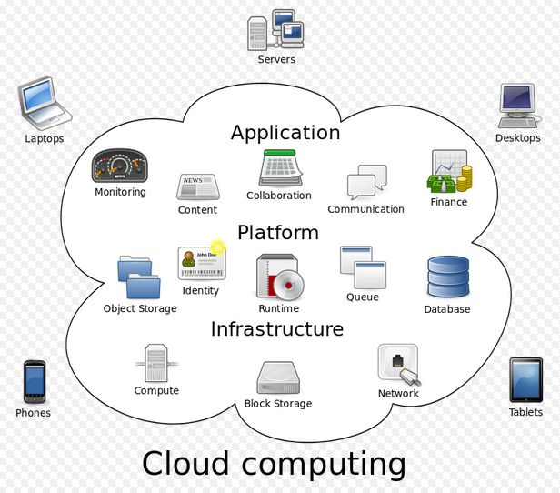
Table of Contents
Chapter 1     Introduction ............................................................................................. 9

Chapter 2     Scenario Description .............................................................................. 11

  2.1   Cloud Computing ........................................................................................... 13

  2.2   Internet of Things .......................................................................................... 17

Chapter 3     Theoretical Background: Big Data, Data Mining, Machine Learning ..... 19

  3.1   Big Data ......................................................................................................... 19

    3.1.1     Big Data Analytics................................................................................... 20

    3.1.2     Data Mining Methods ............................................................................ 20

  3.2   Machine Learning .......................................................................................... 22

    3.2.1     Machine Learning Algorithms ................................................................ 22

    3.2.2     Training Set ............................................................................................ 23

    3.2.3     Supervised, Unsupervised and Semi - Supervised Learning .................. 24

    3.2.4     Data Preprocessing ................................................................................ 24

  3.3   MapReduce and Hadoop Ecosystem ............................................................ 27

Chapter 4     SiteWhere: An Internet of Things Platform ........................................... 32

  4.1   SiteWhere ...................................................................................................... 32

  4.2   Data Visualization .......................................................................................... 36

Chapter 5     Overview of Neural Networks ............................................................... 39

  5.1   Introduction................................................................................................... 39

  5.2   Activation Functions ...................................................................................... 40

  5.3   Neural Network Architectures ...................................................................... 41

    5.3.1     Multilayer Perceptrons .......................................................................... 43

    5.3.2     Long Short - Term Memory .................................................................... 45

Chapter 6     Forecasting based on Neural Networks (NN) techniques ..................... 47

  6.1   Time Series .................................................................................................... 47

                                                                                                                           4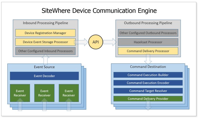
6.2   Results of MLP implementation .................................................................... 48

  6.3   Results of LSTM implementation .................................................................. 55

  6.4   Discussion ...................................................................................................... 64

Chapter 7     Summary ................................................................................................ 66

References 67

                                                                                                                          5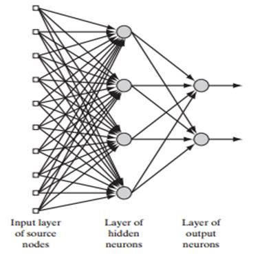
List of Figures

Figure 1: Reims tramway plan. .................................................................................... 12
Figure 2: Cloud computing metaphor [6]. ................................................................... 14
Figure 3: The architecture of cloud computing environment can be divided into 4
layers that are illustrated in above figure [4]. ............................................................. 16
Figure 4: IoT paradigm and the SOA-based architecture for the IoT middleware [1]. 18
Figure 5: Training set derives the model and test set evaluate the final model. ........ 25
Figure 6: MapReduce example [14]. ............................................................................ 28
Figure 7: SiteWhere architecture. [17]. ....................................................................... 33
Figure 8: Diagram of data flow in Communication Engine component [17]. .............. 34
Figure 9: Histograms of the train data as represented by MongoDB Compass. ......... 36
Figure 10: Results of a MongoDB query that was graphically built using MongoDB
Compass. ...................................................................................................................... 37
Figure 11: Map with points of a route of the Reims train. .......................................... 37
Figure 12: Geospatial query graphically built using MongoDB Compass. ................... 38
Figure 13: Graphically results of the geospatial query. ............................................... 38
Figure 14: Non-linear model of a neuron [18]. ............................................................ 40
Figure 15: Feedforward network with a single layer of neuron [18]. ......................... 41
Figure 16: Fully connected feedforward network with one hidden layer and one
output layer [18]. ......................................................................................................... 42
Figure 17: Recurrent Network with hidden neurons [18]. .......................................... 43
Figure 18: Multilayer Perceptrons Network with one hidden layer. ........................... 44
Figure 19: LSTM memory block [6]. ............................................................................. 46
Figure 20: Plots of parameters CO2, Station, Velocity, Acceleration and Power. ....... 48
Figure 21: RMSE metric for different number of epochs for the MLP neural network.
...................................................................................................................................... 49
Figure 22: Plot that illustrates the results of RMSE metric for different batch size for
the MLP neural network. ............................................................................................. 50
Figure 23: Plot that illustrates the results of RMSE metric for different number of
neurons for the MLP neural network with a single hidden layer. ............................... 51

                                                                                                                                       6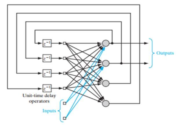
Figure 24: Plot that illustrates the RMSE versus the number of hidden layers for the
MLP neural network. ................................................................................................... 52
Figure 25: Results for different values of window size. The MLP network was
composed of 1 hidden layer with 20 neurons, the number of epochs was 250 and the
batch size was 150. ...................................................................................................... 53
Figure 26: Results for different values of neurons for the stateless LSTM neural
network. The LSTM was composed of 1 hidden layer, the number of epochs was
equal to 1, the batch size equal to 50 and the sequence length equal to 50. ............ 56
Figure 27: Results for different values of neurons for the stateful LSTM neural
network. The LSTM was composed of 1 hidden layer, the number of epochs was
equal to 1, the batch size equal to 50 and the sequence length equal to 50. ............ 56
Figure 28: Results for different lengths of sequence for the stateless LSTM neural
network. The LSTM was composed of 1 hidden layer with 10 neurons, the number of
epochs was equal to 1 and the batch size equal to 50. ............................................... 57
Figure 29: Results for different lengths of sequence for the stateful LSTM neural
network. The LSTM was composed of 1 hidden layer with 15 neurons, the number of
epochs was equal to 1 and the batch size equal to 50. ............................................... 58
Figure 30: Plot that illustrates the RMSE versus the number of hidden layers for the
stateless LSTM neural network. ................................................................................... 60
Figure 31: Plot that illustrates the RMSE versus the number of hidden layers for the
stateful LSTM neural network. .................................................................................... 61
Figure 32: Plot of RMSE values for different subset of features that used as input to
the stateless LSTM neural network. ............................................................................ 63
Figure 33: Histogram plot of RMSE for MLP, stateless LSTM and stateful LSTM (input
power). LSTM models outperformed MLP model and stateful LSTM outperformed
stateless LSTM in terms of error performance. ........................................................... 64
Figure 34:Histogram plot of RMSE for MLP, stateless LSTM and stateful LSTM. (input
subset of features [longitude, latitude, velocity, acceleration] for MLP and feature
acceleration for LSTMs). LSTM models outperformed MLP model and stateful LSTM
outperformed stateless LSTM in terms of error performance. ................................... 65
Figure 35: Histogram plot of RMSE for stateless LSTM and stateful LSTM. (input
acceleration). LSTM stateful outperformed LSTM stateless model. ........................... 65

                                                                                                                           7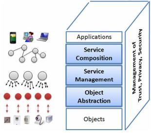
List of Tables

Table 1: Results of RMSE metric for different number of neurons for the MLP neural
network with a single hidden layer.............................................................................. 51
Table 2: Results of RMSE metric for different hidden layers for the MLP neural
network. ....................................................................................................................... 52
Table 3: Comparative 0predictive performance for different values of window size.
The MLP network was composed of 1 hidden layer with 20 neurons, the number of
epochs was 250 and the batch size was 150. .............................................................. 53
Table 4: Results of RMSE metric for different hidden layers for the stateless LSTM
neural network............................................................................................................. 59
Table 5: Results of RMSE metric for different hidden layers for the stateful LSTM
neural network............................................................................................................. 59
Table 6: RMSE values for different subset of features that used as input to the
stateless LSTM neural network. ................................................................................... 62

                                                                                                                                 8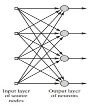
Chapter 1 Introduction

Machine Learning and Cloud Computing are gaining increased popularity over that past
few years. The reason behind this is the rapid increase of the volume of data and the
necessity of their fast processing, in order to extract useful information.

The goal of this master thesis is to investigate the application of machine learning
techniques in support of cloud services. In this work, we focus our effort to improve
the process and analysis of the data of a real railway system (the Reims tramway) by
forecasting the train power consumption. We develop a machine learning technique
based on Neural Networks to process the dataset composed of various physical
quantities related with the Reims tramway, each one measured periodically every
second during the period of a day. The measurements were collected by different sensors,
which were installed on the train. Initially, we provide the required theoretical
background and then we present some relevant experimental results. The theoretical
background involves the introduction of the concept of Big Data, the presentation of
different Data Mining methods and Machine Learning algorithms that can be used in
data processing and a review on Cloud Computing, Internet of Things (IoT) and
SiteWhere.

In Chapter 2, the problem definition is presented and the terms of Cloud Computing
and Internet of Things are introduced. In Chapter 3, we introduce the notions of Big
Data, Data Mining and Machine Learning. In Chapter 4, we begin with the presentation
of the architecture and capabilities of SiteWhere and we conclude with the
visualization of the train data, using a Graphical User Interface (GUI), referred to as
MongoDB Compass. The train dataset was stored in the MongoDB database, which is
supported by the SiteWhere platform. Chapter 5 provides a brief overview of Neural
Networks and the relevant basic algorithms. In Chapter 6 we introduce the concept of
Time Series, implement two different types of Neural Networks, the Multilayer
Perceptrons (MLP) and the Long Short-Term Memory (LSTM) on the train dataset and
we present a set of relevant results.

                                                                                      9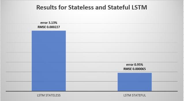
Chapter 7, provides the summary of the thesis and the conclusions derived and
presented in the previous chapters.

                                                                           10
Chapter 2 Scenario Description
The increasing advances in hardware technology, such as the development of
miniaturized sensors, GPS-enabled devices and accelerometers result in greater
access and availability of different kinds of sensor data. This produces the collection
of enormous amounts of data, that can be mined for a variety of analytical insights.
Hence, sensor data introduce a lot of challenges in terms of data collection, storage
and processing. In order to provide ubiquitous and embedded sensing there is a
requirement for data collection from different devices that are connected and
accessible through the Internet. This paradigm is referred to as the Internet of Things
(IoT). The IoT term is used to describe “a world – wide network of interconnected
objects uniquely addressable, based on standard communication protocols” [1] [2],
whose point of convergence is the Internet [3].
In this thesis, we describe and propose the SiteWhere, an IoT platform in order to
collect, store and process data that consists of multiple sensor measurements from
Reims tramway. The Reims tramway plan is depicted in Figure 1. SiteWhere provides the
required functionalities for ingestion, storage, processing and integration of device
data and deal with all above-mentioned challenges caused by sensor data. It also
utilizes datastore technologies, like MongoDB, Apache HBase and InfluxDB to store
data. In this thesis we store the data in the MongoDB database and retrieve, store
locally and process them.
An important problem related with the sensor processing is the multivariate time
series modeling and forecasting. In this work, we focus our effort to improve the
process and analysis of the train’s data, in part by forecasting the train power
consumption. Accurate modeling and prediction of the Reims tramway data is
therefore of great importance and is the motivation behind this thesis.
In Chapter 6, an empirical comparison between MLP and LSTM neural networks is
performed. We consider two different LSTM types and compare their performance
with MLP for making a one step-ahead prediction.
11Figure 1: Reims tramway plan.
The dataset used, is part of a larger dataset, collected from sensors on the Reims
tramway. This part of the dataset contains the following quantities:
i. External Temperature (measurement spot 1)
ii. External Temperature (measurement spot 2)
iii. Longitude
iv. Latitude
v. Station
vi. Velocity
vii. CO2 Level (inside the coaches)
viii. Total Power
122.1 Cloud Computing
With the significant advances in processing and storage technologies and the success
of the Internet the realization of the cloud computing has been enabled. This
computing model, provides the essential computing services to support a wide variety
of services available to organizations, businesses and the public. In the cloud
computing model resources are provided as general utilities that can be leased and
released by users in an on-demand basis [4].
One definition of cloud computing provided by the National Institute of Standard and
Technologies (NIST):
“Cloud computing is a model for enabling ubiquitous, convenient, on-demand network
access to shared pool of configurable computing resources (e.g., networks, servers,
applications, and services) that can be rapidly provisioned and released with minimal
management effort or service provider interaction [5].”
In the context of cloud computing the elements of the network representing the
rendered services are invisible to the end users, as if it is obscured by a cloud [6]. This
concept is depicted in Figure 2.
13Figure 2: Cloud computing metaphor [6].
The cloud model is composed of five cloud computing characteristics, three different
service models and four types of clouds [5].
Cloud Computing Characteristics
1. On demand self-service. A consumer can allocate or deallocate computing
resources automatically, in an on-demand fashion without requiring human
interaction. This automated resource management attains high performance
and agility.
2. Broad network access. Computing capabilities are accessible through the
Internet. Hence cloud services are available to be used by any device with
Internet connectivity (e.g. mobile phones, tablets, and laptops).
143. Resource pooling. The provider’s computing resources are pooled, thus they
can be dynamically assigned and reassigned to multiple resource consumers
according to demand. Each costumer can specify the location of the provided
resources only at a higher level of abstraction (e.g. country, state, or
datacenter) while he is not able to know the exact location.
4. Rapid elasticity. Computing capabilities are elastically provisioned and
released in order to scale rapidly in accordance to the level of demands.
5. Measured services. Cloud computing employ a pay-per-use model, so
computer systems ought to use a metering capability at some level of
abstraction vary from service to service. As a result, resource usage can be
monitored, controlled and reported providing transparency for both the
provider and resource consumer.
Service Models
1. Software as a Service (SaaS). The consumer is capable to use the provider’s
applications. These applications are accessible from various client devices and
are running on a cloud infrastructure.
2. Platform as a Service (PaaS). The resources provided to the consumer include
operating system support and software development frameworks. Therefore,
the consumer is able to deploy onto the cloud infrastructure consumer-
created or acquired applications created using programming languages,
libraries, services and tools.
3. Infrastructure as a Service. IaaS provide various computing resources (e.g.
processing, storage, and networks) where arbitrary software can be deployed
and run by the consumer.
15Types of clouds
1. Private cloud. Private clouds are offered for exclusive use by a single
organization. They may be built and managed by the organization or other
external providers. It may exist on or off premises of cloud provider.
2. Community cloud. Community clouds are designed for exclusive use by a
specific community of organizations that have shared concerns. It may be built
and managed by one or more organizations in the community or by external
providers. It may exist on or off premises of cloud provider.
3. Public cloud. A public cloud can be used by the general public and it may be
built and managed by a business, academic, or government organization, a
third party or combination of them. It exists on the premises of the cloud
provider.
4. Hybrid cloud. Hybrid cloud is a combination of two or more cloud
infrastructures (e.g. private, community, or public). In a hybrid cloud the
entities preserve their uniqueness.
Figure 3: The architecture of cloud computing environment can be divided into 4 layers that are
illustrated in above figure [4].
162.2 Internet of Things
The IoT term is used to describe “a world – wide network of interconnected objects
uniquely addressable, based on standard communication protocols” [1] [2], whose
point of convergence is the Internet [3]. These objects are able to identify, measure
and modify the physical environment acting as sensors and actuators.
aspects that are related to the Internet of Things are the Radio Frequency
Identification (RFID), the sensor networks, the addressing and the middleware.
RFID systems are attached to objects to provide the automatic identification of them
and allow them to be assigned to unique digital identities, to be integrated into a
network and to be associated with digital information and services [3]. RFID systems
composed of two parts, the transponders, also known as RFID tags, and the readers.
The RFID tags are small microchips that comprise a memory to store electronically
information and an antenna. They can be active, passive or battery-assisted passive.
The active tags have battery, so they periodically transmit ID signals. In contrast,
passive tags have no battery, so they use only radio energy transmitted by the reader.
Finally, if tags are battery-assisted passive, they transmit ID signals when a RFID reader
appears. The RFID readers usually trigger the tag transmission by generating an
appropriate signal, querying for possible presence of tags and for the reception of
their unique IDs [1].
Sensor networks along with RFID systems contribute to gain more information about
the status of things, since they are capable to take measurements and get information
about the location, movement and temperature. Sensor networks can be composed
of a large amount of sensing nodes that can communicate to each other in a wireless
network. Wireless sensor networks (WSNs) may provide useful data and are used in
several application scenarios. However, WSNs and generally sensor networks have to
tackle many communication and resources problems, such as short communication
range, security, privacy, power considerations, storage, processing capabilities and
bandwidth availability.
17Addressing refers to the ability to uniquely identify the interconnected objects. This
issue is very crucial for the success of IoT since this allows to uniquely address a huge
number of devices and control them through the Internet [3].
Middleware is a software layer between the object and the application layer
composed of three subs–layers, known as object abstraction, service management
and service composition layer. These sub—layers are utilized in order to face the
heterogeneity of the participating objects, their limited storage and limited processing
capabilities and the large amount of applications that are included in the application
layer. In addition, middleware has to deal with security issues and provide
functionalities that manage the privacy and security of all the exchanged data. These
functions could be included in an additional layer or distributed through the stack
between the object abstraction and service composition layer. The last solution is used
more often. An IoT paradigm and the SOA-based architecture for the IoT middleware
are depicted in the Figure 4.
Figure 4: IoT paradigm and the SOA-based architecture for the IoT middleware [1].
18Chapter 3 Theoretical Background: Big Data,
Data Mining, Machine Learning
The goal of this chapter is to provide the basic definitions, properties and tools which
are related with the concept of Big Data, Data Mining and Machine Learning. These
terms are often used interchangeably, so it is decided to discuss these in the same
chapter. Hadoop and all the components included in the Hadoop ecosystem are
significant tools correlated with Big Data. The essence of data mining and machine
learning are introduced and various data mining methods and machine learning
algorithms are summarized. Data mining is the process of learning patterns and
identifying predictive models from large-scale datasets. It usually uses machine
learning algorithms in order to extract valuable information from the data.
3.1 Big Data
A widely used definition of Big Data is derived from Gartner. In 2012, Gartner defined
the exploding amount of data as follows:
“Big data is high volume, velocity, and/or variety information assets, that require
new forms of processing to enable enhanced decision making, inside discovery and
process optimization [7].”
According to the above definition one understands that volume, velocity and variety
are three basic characteristics of the big data. The terms volume, velocity and variety
referred to the huge amount of data, the speed that data are stored, managed and
manipulated at the right time and the variety of data sources, types and structures
respectively.
193.1.1 Big Data Analytics
Big data analysis is the data mining field that aims to manage fast vast amounts of
data. In this section, we summarize different types of data analytics.
Big data analytics are separated into two types, basic analytics and advanced analytics.
Basic analytics are used to investigate the data and it may include visualizations or
simple statistics. Some significant operations of basic analytics involve: the division of
data into smaller sets of data that ease the examination of them, the track of large
volumes of data in real time, and the anomaly detection, for example an event with
actual observation different from expected.
On the contrary, advanced analytics provide some algorithms and a lot of data mining
techniques, such as innovative statistical models, neural networks and other machine
learning methods for more complicated analysis. Some examples of advanced
analytics include: predictive models composed of algorithms and techniques used on
large volume of data to predict future outcomes, text analytics and other statistical
and data mining methods and algorithms, like forecasting, classification, clustering
and optimization. Nowadays, advanced analytics are becoming increasingly famous,
because they achieve substantial power increase and enable new algorithm
development that makes the manipulation of big data easier and more efficient.
3.1.2 Data Mining Methods
As mentioned in the previous paragraph, advanced analytics utilize various data
mining techniques. Data mining is a computing process that includes basic algorithms
and methods that enable gaining knowledge from big data. In fact, it is a part of a
wider knowledge investigation process, which comprises preprocessing and
postprocessing tasks. Some examples of preprocessing tasks are data extraction, data
cleaning, data fusion, data reduction and feature construction, while some examples
of postprocessing tasks are pattern and model explanation, data visualization and
online updating. Data mining is an interdisciplinary subfield that merges concepts
from database systems, statistics, machine learning and pattern recognition [8].
20Some basic data mining postprocessing methods are presented below.
Classification
The goal of the classification process is to assign an unknown item to one of some
predefined classes. This is achieved by defining a function f based on a training set
that comprises many items and their corresponding class. The function defined by the
training set is called classifier. After the classifier is trained, it is possible to predict the
class of any unknown item. As far as machine learning goes, perspective classification
is a supervised learning.
Regression
Contrary to classification process, in regression analysis the output variable takes
values in an interval in the real axis. Hence, given a training set, the task is to estimate
a function f, whose graph fits the data. After this function is estimated, an unknown
input point can be assigned to a specific output value [9].
Clustering
Clustering is the problem of partitioning data into groups so that each group contains
similar objects. The more similar the objects within a group are to each other and
more dissimilar from the objects in other groups, the better the clustering is. In terms
of machine learning, the exploration of clusters is an unsupervised learning because
cluster analysis needs to capture the hidden structure from unlabeled data in order to
group them.
Forecasting
Forecasting is a process of making predictions of future values of a variable based on
past and present observations. The term prediction is similar to forecasting. The main
difference between them is that forecasting is used for the estimation of values at
specific future times, while prediction is used for more general estimations [10].
213.2 Machine Learning
As it has been already mentioned in the introductory paragraph, the data mining
process usually uses machine learning algorithms. In this section, we will explain the
basic concepts someone needs for a full understanding of machine learning by
introducing basic definitions and different kinds of machine learning algorithms.
3.2.1 Machine Learning Algorithms
Machine learning algorithms can be separated into groups depending on the form by
which the function f is represented. Below we present the most popular machine
learning algorithms.
Decision trees: In this category, the form of the function f is a tree. Decision trees
are a collection of nodes, each of which has a function f of x . There is a root node,
interior nodes and the leaves nodes (nodes that don’t have children). To classify a
feature vector x , we start from the root node and according to the value of f x we
decide to which child or children the search must proceed. The classification task is
completed when a leaf is reached. Decision trees are suitable for binary and multiclass
classification and regression problems. Some examples of decision tree algorithms are
the Classification and Regression Tree, the Iterative Dichotomizer3, the Decision
Stump and Conditional Decision Trees.
Perceptrons: Perceptron is a function which is associated with a vector of weights
w w1 , w2 , w3 ,..., wn with real valued components and applied to a feature vector
x x1 , x2 , x3 ,..., xn with real valued components, too. Perceptron has a threshold .
The output of the perceptron is equal to +1 if the inner product w x is grater that
threshold or otherwise it is equal to -1. Perceptron is suitable for binary
classification [11].
22Neural nets: Neural nets are networks composed of layers, each of which contains one
or more perceptrons. The output of some perceptrons can be used as input to next
layer’s perceptrons. Neural nets are suitable for binary or multiclass classification.
Multiclass classification is supported since many perceptrons can be used as outputs
by associating each of them with a specific class. More details about neural nets are
given in Chapter 5.
Instance – based learning algorithms: An instance – based algorithm uses a similarity
measure to compare new feature vectors with the data seen during the training
procedure. According to the results of the comparison, it makes predictions and
classifies new data properly. An important kind of instance based algorithms is the k-
Nearest Neighbor algorithm (kNN).
Support – vector machines: The goal of support vector machines is to find a
hyperplane w x b 0 that separates the points of the training set into two classes
and maximizes the distance between the hyperplane and the points simultaneously.
Support vectors are the points that are at distance from the hyperplane [11].
Support vector machines are used for classification and regression analysis.
3.2.2 Training Set
The training set contains the data that are given to machine learning algorithms for
learning. It comprises a set of pairs x, y , where x is a vector of categorical or
numerical values, known as feature vector and y is the label that denotes the class in
which x belongs. There are many types y of that define the type of the machine
learning problem. To be more specific, if y is a real number, then the machine learning
problem is a regression problem. In contrast, if label y is a Boolean value -1 (false) or
+1 (true) or a member of some finite set, then the machine learning problem is a
binary or a multiclass classification problem respectively. Finally, the label y may be a
member of potentially infinite set, such as a parse tree for x [11].
233.2.3 Supervised, Unsupervised and Semi - Supervised
Learning
Machine learning can be categorized into supervised, unsupervised and semi –
supervised depending on the type of the given training set.
Supervised learning: the training set is composed of input variables x1 , x2 , x3 ,..., xn ,
known as features and output variables y1 , y2 , y3 ,..., yn , known as labels. In this case,
the algorithm learns how to map each input xi to the corresponding label y j and
designs a function, which is capable of predicting the output label given any new input.
Some supervised learning algorithms are the linear regression, random forest and
support vector machines.
Unsupervised learning: the training set comprises only the input variables
x1 , x2 , x3 ,..., xn and no corresponding labels. The unsupervised learning algorithms
have to model the structure or the distribution in the input data. Some examples of
unsupervised machine learning algorithms are the clustering and the association rule
problem.
Semi – supervised learning: the training set is composed of a large amount of
unlabeled input data. In semi – supervised learning class only a small percentage of
the input data include their corresponding labels.
3.2.4 Data Preprocessing
Data preprocessing is required before machine learning algorithms are applied to
training sets, because the quality of the data and the information that they contain
are two factors that affect the learning performance. Below we present some needful
preprocessing techniques. Some of them will be used in Chapter 6.
Missing values: missing values in real world datasets are a common incident that
reduce the representativeness of the samples and can cause unpredictable results if
they are ignored. There are several preprocessing techniques to treat the missing
data, like mean imputation or simply removing the features or samples that contain
24missing values. To eliminate features and samples with missing values is a convenient
approach, but if many features or samples are removed from dataset, it can lead to
the loss of valuable and useful information. In contrast, mean imputation is a safer
approach. Mean imputation is an interpolation technique that substitutes missing
values by the mean value of the total feature column.
Training set and test set: Dividing dataset into training and test set is an effective
approach to avoid overfitting. Overfitting occurs when the machine learning algorithm
performs well only on the training set, but it is unable to generalize well to new data.
So, to avoid overfitting the training set is used to train and optimize the model, while
the test set is used to estimate the accuracy of the final model and indicate if the
model is overfitting the data. The separation of the dataset into training and test set
must reserve the valuable information in the training set. However, smaller test sets
may lead to less accurate estimation of the generalization error. The most commonly
used splits are 60-40, 70-30 or 80-20 calculate on size of the initial dataset.
Figure 5: Training set derives the model and test set evaluate the final model.
Feature scaling: Feature scaling is an essential step in data pre-processing, since
machine learning algorithms behave better if the values of feature vectors are on the
same scale. We present an example to understand the importance of feature scaling
in machine learning.
Example: If there are two features, one of which is measured on scale from 1 to 10
and the second on scale from 1 to 100,000, then the squared error function in a
25classifier will focus on optimizing the weights to larger errors in the second feature
[12].
The well-known techniques for feature scaling are the normalization and
standardization techniques.
In normalization, the min – max scaling is applied to each feature column, so that each
i
sample xi is replaced by the new value xnorm , where xnorm is calculated as follows:
xi xmin
i
xnorm , where xi is a particular sample, xmin is the minimum value in the
xmax xmin
feature vector and xmax is the maximum value in the feature vector.
Standardization is a technique that can be more practical for many linear models
which are used to initialize weights to zero or small random values close to zero. It
centres the feature columns at mean zero with standard deviation equal to one, thus
the feature columns take the form of a normal distribution which in turns eases the
algorithm to learn the weights. In addition, standardization makes the algorithms less
i
sensitive to outliers by holding useful information about them. The new value xstd of
each sample xi is calculated as follows:
xi x
i
xstd , where x is the sample mean of a particular feature vector and x the
x
corresponding standard deviation [12].
Regularization: The goal of a machine learning algorithm is to find a set of weight
coefficients that minimizes the error on the training data. Regularization is a
preprocessing technique that adds a penalty term to the initial error in order to
penalize complex models. Finally, instead of the error on the data, the learning
algorithm must minimize an augmented error which is given by the equation:
E error on data mod el complexity
The parameter gives the weight of the penalty term [13].
26Dimensionality reduction: Feature selection and feature extraction are two
fundamental techniques for dimensionality reduction. In feature selection, algorithms
intend to create a subset composed of the most relevant to the problem original
features and remove the irrelevant features. In this way, they achieve to reduce the
dimensions of the initial feature subspace. In feature extraction, algorithms derive the
valuable information from the initial dataset and project the data onto a new feature
subspace of lower dimensionality. Feature extraction can be understood as data
compression with the goal of maintaining most of the relevant information [12]. The
Principal Component Analysis (PCA) and Linear Discriminant Analysis (LDA) are basic
algorithms that are widely used for feature extraction and dimensionality reduction.
3.3 MapReduce and Hadoop Ecosystem
In this part, we will outline the MapReduce model and other tools, like Apache Hadoop
and the Hadoop-related Apache projects Pig, Hive, HBase and Mahout. Big data
analysis requires large amount of data to be managed with high speed. Computing
clusters and Distributed File Systems (DFS), enable the parallelization of various
operations, like computations and data transfer. Based on the DFS, many higher-level
programing systems have been developed, with most significant the MapReduce
system.
MapReduce
MapReduce is a programing model, that is used for data administration and
processing. It is composed of two functions, the Map and the Reduce functions. The
Map function applies an operation to a specific part of data and provides a set of
intermediate key/value pairs. The Reduce function takes an intermediate key and a
set of values related with that key, merges together these values and provides the
final output.
The simplest example to get an understanding of MapReduce is the word count
example, in which the only operation is to count how many times each word appears
in a collection of documents. In other words, the task is to create a list of words and
27identify the frequency with which they appear in order to find the relative importance
of certain words. In the following example, the input of the Map function is a line of
text. At first, the Map function analyses the text string into individual words and
produces a set of key/value pairs of the form . Finally, the Reduce function
sums up the 1 values and provides the pair, which is the final output.
The MapReduce example is illustrated in Figure 6 [14].
Figure 6: MapReduce example [14].
Apache Hadoop
Apache Hadoop is a project which develops open-source software for reliable,
scalable, and distributed computing [15]. Hadoop successfully executes the operations
of the MapReduce model at a high level. The base of Hadoop is the Hadoop Distributed
File System (HDFS), in which data are distributed through a computing cluster. HDFS
separates each file into fixed size blocks and stores them across a computing cluster.
In addition, it creates three replicates of each block, that are stored on different nodes
in the Hadoop cluster. As a result of replicates, Hadoop is capable of responding even
in the case of a hardware failure and it is more flexible in determining which machine
to use for the map step on a specific block. The manipulation of the data access in
HDFS is accomplished by three background processes, usually called Java Daemons,
each of which has a particular task. The three Java Daemons are known as Name Node,
Data Node and Secondary Name Node. Name Node determines where the blocks of
data are stored on a single machine, Data Node manages the stored data on each
28machine and the Secondary Name Node can perform some of the Name Node tasks
in order to reduce its workload. Machines are classified into two categories by
processes that they run. The first category is the master nodes and the second
category is the worker nodes. Master nodes run the Name Node and the Secondary
Name Node while worker nodes run the Data Nodes.
Apache Pig
Apache Pig is a high-level platform that contains an environment to execute the Pig
code and a data flow language, called Pig Latin. The main advantage of Pig is the
simplicity of developing and executing a MapReduce task. Pig instructions are
translated into MapReduce jobs in background. Additionally, in Pig the execution of
several common data manipulations, such as inner and outer joins between files, is
the same as that of the SQL language used in a relational database. Finally, Pig
language can be extended using user-defined functions (UDFs), thus some operations
can be coded in other programing languages, for instance Python, JavaScript or
Groovy, and then executed in the Pig environment [14].
Apache Hive
Apache Hive is a data warehouse structure built on top of Hadoop that provides data
summarization, query and analysis [16]. The language of Hive is the HiveQL (Hive
Query Language) and it is like the SQL language. Hive provides table structures with
rows and columns. Each row represents a record, transaction or a particular entity.
The value of the corresponding column represents the attribute of the row. Hive is a
good tool to be used if the table is the appropriate structure for data visualization.
However, Hive is not the suitable tool for real – time queries because a Hive query has
to be translated into a MapReduce job and then submitted to the Hadoop cluster [14].
Apache HBase
Apache HBase is Hadoop database, that provides real-time read and write access to
the big data. The HBase design is based on Google's 2006 paper on BigTable [14]. It is
constructed upon HDFS. HBase achieves real-time operations very quickly by dividing
29the workload over different nodes in a distributed cluster. More specifically, each
table is separated into a few regions and a worker node is responsible for a specific
range of data in the table column. As the table size increases or the user load
increases, additional nodes and region splits can be added to scale the cluster
properly. The form that the contents are stored on an HBase table is a key/value form.
The values represent the data stored at the intersection of the row, column and
version. The key contains the next elements:
1. Row
2. Row length
3. Column family
4. Column family length
5. Column qualifier
6. Version
7. Key type
Row is used as the primary attribute to access the data of an HBase table. The way
that data are distributed depends on it, so the structure of the row has to be designed
according to how the data will be accessed.
Column family provides grouping for the column qualifiers.
Version or timestamp make it possible to maintain different values of the contents in
an intersection of a row and a column.
Key type indicates whether a write operation corresponds to add data into the HBase
table or delete data from the table [14].
Apache Mahout
Apache Mahout provides executable Java code that implements various machine
learning algorithms and data mining techniques, that can be used for big data analysis.
It contains classification algorithms, such as Logistic Regression, Naïve Bayes, Random
forests and Hidden Markov models. It also contains clustering algorithms, like canopy,
K-means, fuzzy K-means, dirichlet, mean-shift and some recommenders -
30collaborative filtering, such as non-distributed recommenders and distributed item-
based collaborative filtering.
31Chapter 4 SiteWhere: An Internet of Things
Platform
In the beginning of this chapter we describe SiteWhere, an Internet of Things solution
used to manage and analyze device data. The next topic presented in this chapter is
data visualization, which is performed using a GUI for MongoDB database, the
MongoDB Compass.
4.1 SiteWhere
The middleware solutions discussed above are referred to as IoT platforms. In this
section, we will focus our attention to SiteWhere, an open source Internet of Things
platform that provides all the required functionalities for ingestion, storage,
processing and integration of device data.
The core of SiteWhere relies on many proven and open source technologies in order
to carry out all the required functions mentioned in the previous paragraph. An
important technology adopted is that of the Tomcat Server, a java servlet container in
which SiteWhere runs as a Web Application Archive (WAR) file. Some other
technologies are the Spring Framework, Spring Security and Hazelcast. In addition,
SiteWhere utilizes datastore technologies, like MongoDB, Apache HBase and InfluxDB
to store data. Finally, it uses complementary technologies like the Mule AnyPoint
Platform and Apache Spark.
SiteWhere architecture is illustrated in Figure 7. It consists of various components that
will be analyzed further in the following paragraphs.
32Figure 7: SiteWhere architecture. [17].
A significant component is the SiteWhere Server, a central component which controls
all other system’s components and the processing of device data.
Another component is the Tenant Engine. A specific SiteWhere instance is capable to
have multiple tenants and thus to serve multiple IoT applications. Each system tenant
can have different data storage and processing pipeline without affecting other
tenants. In addition, it is configured to communicate with devices over any number
of most popular communication protocols, like Message Queue Telemetry Transport
(MQTT), Advanced Message Queuing Protocol (AMQP) and Stomp. Although the
default communication protocol is the MQTT.
Communication engine is a component that is encapsulated in the Tenant Engine. It
ensures the internal event handling. Its operations are the registration of new or
existing devices, the receipt of events from connected devices and the delivery of
commands to them.
33It is also important to mention that events are the core data that SiteWhere revolves
around. SiteWhere manages different types of events such as measurements,
locations, alerts and command invocations and responses.
Figure 8 illustrates the flow of data in the Communication Engine component.
Figure 8: Diagram of data flow in Communication Engine component [17].
SiteWhere is able to send and receive data either from devices or from other agents
via Representational State Transfer (REST) services. REST services can be used by
authenticated users to create, view, update or delete entities in the system. They can
also be used by devices and directly interact with SiteWhere.
In addition, SiteWhere cooperates with NoSQL databases to store and retrieve the
data that are collected from devices. MongoDB, Apache HBase and the InfluxDB are
three databases which supported by SiteWhere. The MongoDB is a document
oriented database with great performance, availability and high scalability. The HBase
database is a NoSQL and distributed database in which device events are stored as
time series data. A brief description of HBase has already been pointed out in Chapter
3. The InfluxDB is a time series database that supports advanced clustering and
provide high scalability. The InfluxDB database also provides a tool for data
visualization, reffered to as Grafana [17].
34Furthermore, SiteWhere facilitates the integration with other platforms through
Hazelcast, an in-memory data grid. This way, SiteWhere’s functionalities and
capabilities can be improved and extended.
Another important feature of SiteWhere is its capability to support several external
device platforms. These include the Android Development Kit, the Arduino
Development Kit and the Java Agent. As a result, the interaction and the interchange
of events between the server and the Android devices, Arduino devices or Java agents
are easy to take place. Moreover, the Mule AnyPoint Platform and the Apache Spark
are two external platforms that can connect to a SiteWhere server instance and
exchange data with it via Hazelcast services. The Mule AnyPoint is an ESB platform
which manages interactions across varied systems since it supports a lot of
communication protocols and the Apache Spark is a computing framework which is
used to large – scale data processing.
Finally, SiteWhere makes it easy to associate the devices with physical assets, like
people, places and things and describe the hardware information or configuration.
Each device can be registered along with its unique hardware id and device specific
metadata [17].
In summary, SiteWhere is a platform suitable to support the work of this thesis.
SiteWhere can be used to facilitate network connectivity of train sensors. Through this
sensor measurements can be stores in the MongoDB database of SiteWhere. If the
data are stored, can then be retrieved and stored locally allowing their offline
processing. In Chapter 6 we propose the use of Neural Networks for forecasting using
the sensor data retrieves from the MongoDB database and present some relevant
experimental results. If the sensors are connected to SiteWhere, Neural Networks can
be adopted and used for real time forecasting via services provided by Hazelcast.
Finally, data visualization providing immediate insight into the server status and query
performance can be also provided, using various visualization tools. In the next
section, we will use the MongoDB Compass and visualize the train data that we have
stored in the MongoDB database.
354.2 Data Visualization
The database that was used in this thesis to store the collected train data was
MongoDB. We also used MongoDB Compass for data visualization. MongoDB
Compass is a graphical tool introduced by MongoDB.
It allows the user to analyze and visualize its database scheme through histograms,
which represent the frequency of the data and their distribution in a collection. Figure
9 illustrate the histograms of the train data that are stored in a MongoDB database.
Figure 9: Histograms of the train data as represented by MongoDB Compass.
36In addition, MongoDB Compass makes easier the MongoDB queries. Users can simply
click on the chart or on a range of charts of the data histogram and as a result a
MongoDB query will be automatically built in the query bar. Figure 10 shows results
of a query about the CO2 that was graphically built using MongoDB Compass.
Figure 10: Results of a MongoDB query that was graphically built using MongoDB Compass.
Finally, MongoDB Compass can use the geospatial functions provided by MongoDB. If
a geospatial index introduced in the MongoDB collection, the MongoDB Compass
shows a map with identified the points of interest. This map is illustrated in Figure 11.
To create the geospatial data depicted below we combined the latitude and longitude
data from the collected train dataset.
Figure 11: Map with points of a route of the Reims train.
37Since geospatial data are supported by MongoDB Compass, users are able to build
geospatial queries and extract the results graphically and as a JSON documents.
Figure 12 shows the implementation of a query and Figure 13 shows the graphical
results for the location and the power consumption of the train.s
Figure 12: Geospatial query graphically built using MongoDB Compass.
Figure 13: Graphically results of the geospatial query.
38Chapter 5 Overview of Neural Networks
In this chapter, we provide an overview of Neural Networks. We introduce the
different Neural Networks’ architectures and some algorithms related to them, such
as the backpropagation and gradient descent algorithm. Finally, we analyze further
the Multilayer Perceptrons and the Long Short-Term Memory neural network.
5.1 Introduction
Before trying to give a definition of Artificial Neural Networks, we will provide a review
of biological brain. The human brain consists of many interconnected neurons.
Neurons are computational cells, that are responsible for processing, transmitting
signals and accomplishing recognition tasks. “Warren McCullock and Walter Pitts
published the first concept of a simplified brain cell, the so-called McCullock-Pitts
(MCP) neuron, in 1943”. Warren McCullock and Walter Pitts correlated the nerve cell
with the logic gate. These logic gates get chemical and electrical signals as input and if
they exceed a threshold, then a specific output signal is generated [12].
Artificial Neural Networks, that are usually referred to as “Neural Networks”, are a
replica of Biological Neural Networks. Neural Networks are composed of a group of
interconnected computational units, that are called neurons and they can interact
with the environment. The knowledge is stored in synaptic weights by interneurons
connection strengths. Finally, knowledge is accomplished through a learning
algorithm. A learning algorithm is a function that updates the synaptic weights during
the learning operation [18].
There are three basic elements of the neural model:
1. A collection of synapses or connecting links between neurons. Each synapse
has its own weight.
2. An adder for summing the neuron’ s input signals. Before summing, each signal
has been multiplied by the corresponding synaptic weight. The aggregation is
linear.
39You can also read