Fractional snow-covered area: scale-independent peak of winter parameterization - DORA 4RI
←
→
Page content transcription
If your browser does not render page correctly, please read the page content below
The Cryosphere, 15, 615–632, 2021
https://doi.org/10.5194/tc-15-615-2021
© Author(s) 2021. This work is distributed under
the Creative Commons Attribution 4.0 License.

Fractional snow-covered area: scale-independent peak
of winter parameterization
Nora Helbig1 , Yves Bühler1 , Lucie Eberhard1 , César Deschamps-Berger2,3 , Simon Gascoin2 , Marie Dumont3 ,
Jesus Revuelto3,4 , Jeff S. Deems5 , and Tobias Jonas1
1 WSL    Institute for Snow and Avalanche Research SLF, Davos, Switzerland
2 Centre  d’Etudes Spatiales de la Biosphère, UPS/CNRS/IRD/INRAE/CNES, Toulouse, France
3 Univ. Grenoble Alpes, Université de Toulouse, Météo-France, CNRS, CNRM,

Centre d’Études de la Neige, 38000 Grenoble, France
4 Instituto Pirenaico de Ecología, Consejo Superior de Investigaciones Científicas (IPE–CSIC), Zaragoza, Spain
5 National Snow and Ice Data Center, University of Colorado, Boulder, CO, USA

Correspondence: Nora Helbig (norahelbig@gmail.com)

Received: 3 August 2020 – Discussion started: 27 August 2020
Revised: 28 December 2020 – Accepted: 30 December 2020 – Published: 9 February 2021

Abstract. The spatial distribution of snow in the mountains     gests that the new parameterizations perform similarly well
is significantly influenced through interactions of topogra-    in most geographical regions.
phy with wind, precipitation, shortwave and longwave radia-
tion, and avalanches that may relocate the accumulated snow.
One of the most crucial model parameters for various ap-
plications such as weather forecasts, climate predictions and   1   Introduction
hydrological modeling is the fraction of the ground surface
that is covered by snow, also called fractional snow-covered    Whenever there is snow on the ground, there will be large
area (fSCA). While previous subgrid parameterizations for       spatial variability in snow depth. In mountainous terrain, this
the spatial snow depth distribution and fSCA work well, per-    spatial distribution of snow is significantly influenced by to-
formances were scale-dependent. Here, we were able to con-      pography due to corresponding spatial variations in wind,
firm a previously established empirical relationship of peak    precipitation, and shortwave and longwave radiation and in
of winter parameterization for the standard deviation of snow   steep terrain due to avalanches that may relocate the accu-
depth σHS by evaluating it with 11 spatial snow depth data      mulated snow. As a result, the snow-covered landscape can
sets from 7 different geographic regions and snow climates      consist of a complex mix of snow-free and snow-covered ar-
with resolutions ranging from 0.1 to 3 m. An enhanced per-      eas, especially in steep terrain or during snowmelt. A param-
formance (mean percentage errors, MPE, decreased by 25 %)       eter which describes how much of the ground is covered by
across all spatial scales ≥ 200 m was achieved by recalibrat-   snow is the fractional snow-covered area (fSCA). Most of
ing and introducing a scale-dependency in the dominant scal-    the time, fSCA is tightly linked to snow depth (HS) and in
ing variables. Scale-dependent MPEs vary between −7 %           particular to its spatial distribution. A fSCA is able to bridge
and 3 % for σHS and between 0 % and 1 % for fSCA. We            the spatial mean HS and the actual observed snow coverage.
performed a scale- and region-dependent evaluation of the       Sound fSCA models are therefore crucial since for the same
parameterizations to assess the potential performances with     spatial mean HS in early winter and in late spring, the as-
independent data sets. This evaluation revealed that for the    sociated fSCA can be completely different (e.g., Luce et al.,
majority of the regions, the MPEs mostly lie between ±10 %      1999; Niu and Yang, 2007; Magand et al., 2014).
for σHS and between −1 % and 1.5 % for fSCA. This sug-             A fSCA plays a key role in modeling physical processes
                                                                for various applications such as weather forecasts (e.g.,
                                                                Douville et al., 1995; Doms et al., 2011), climate simula-

Published by Copernicus Publications on behalf of the European Geosciences Union.
616                                                                             N. Helbig et al.: Fractional snow-covered area

tions (e.g., Roesch et al., 2001; Mudryk et al., 2020) and          ter equivalent (SWE) by a so-called snow-cover depletion
avalanche forecasting (Bellaire and Jamieson, 2013; Horton          (SCD) curve. SCD curves were originally introduced in mod-
and Jamieson, 2016; Vionnet et al., 2016). As climate warms,        els without taking into account subgrid topography or vegeta-
fSCA is an highly relevant indicator for spatial snow-cover         tion. In principle, there are two commonly applied forms: so-
changes in climate projections (e.g., Mudryk et al., 2020).         called closed functional forms and parametric probabilistic
A decrease in spatial snow extent prominently changes sur-          SCD curve formulations (Essery and Pomeroy, 2004). Para-
face characteristics, such as albedo in mountain landscapes,        metric SCD curves have disadvantages for practical appli-
leading to changes in surface radiation, which is a primary         cations such as numerical stability, computational efficiency
component of the surface energy balance. A fSCA is also a           and assuming an unimodal distribution which might be less
parameter in hydrological models to scale water discharges          appropriate for large grid cells covering heterogeneous sur-
appropriately to help manage basin water supply (e.g., Luce         face such as mountainous terrain (e.g., Essery and Pomeroy,
et al., 1999; Thirel et al., 2013; Magnusson et al., 2014;          2004; Swenson and Lawrence, 2012). Various closed func-
Griessinger et al., 2016). Errors in fSCA estimates directly        tional forms for fSCAs are therefore applied in land sur-
translate into errors of snowmelt rates and melt water dis-         face and climate models (e.g., Douville et al., 1995; Roesch
charge (Magand et al., 2014). Thus, accurately describing fS-       et al., 2001; Yang et al., 1997; Niu and Yang, 2007; Su
CAs is of key importance for multiple model applications in         et al., 2008; Swenson and Lawrence, 2012). Most of these pa-
mountainous terrain where highly variable spatial snow dis-         rameterizations use simple relationships between fSCA and
tributions occur.                                                   spatial mean HS or SWE. Since topography strongly deter-
   A fSCA can be obtained from satellite remote sensing             mines the spatial snow depth or snow water equivalent dis-
products using optical imagery with varying spatiotemporal          tribution (Clark et al., 2011), in the past, terrain character-
resolutions. For instance, Sentinel-2 gathers data at a spa-        istics were mostly heuristically introduced in closed form
tial resolution of 10 to 20 m at frequent global revisit inter-     curves to account for subgrid terrain influences on fSCA
vals (< 5 d, cloud permitting) (Drusch et al., 2012; Gascoin        (e.g., Douville et al., 1995; Roesch et al., 2001; Swenson
et al., 2019). The availability of satellite-derived fSCA re-       and Lawrence, 2012). To verify the commonly applied closed
mains, however, inconsistent due to time gaps between satel-        forms of fSCA, Essery and Pomeroy (2004) integrated log-
lite revisits, data delivery and the frequent presence of clouds    normal SWE distributions and fitted the parametric SCD
which obscure the ground, especially in winter in mountain-         curves. The best fit obtained resulted in a function propor-
ous terrain, thus reducing the availability of images drasti-       tional to tanh, which is a previously derived closed form from
cally (e.g., Parajka and Blöschl, 2006; Gascoin et al., 2015).      Yang et al. (1997). By using a normal probability density
Satellite-derived fSCAs can also not be used directly for fore-     function (pdf), Helbig et al. (2015) obtained the same form
casting. Alternatively, fSCAs can be obtained from spatially        fit for fSCA as Essery and Pomeroy (2004). The functional
averaging by using snow models at subgrid scales. While             form for fSCA from Yang et al. (1997) could thus be in-
such snow-cover models are available (e.g., Tarboton and            ferred from integrating normal, as well as log-normal, snow
Luce, 1996; Marks et al., 1999; Lehning et al., 2006; Essery        depth distributions with subsequent fitting of the parametric
et al., 2013; Vionnet et al., 2016), up until now they could not    SCD curves. The main difference between the form of Yang
be used at very high spatial resolutions over very large re-        et al. (1997) and Essery and Pomeroy (2004) is the variable
gions in part due to a lack of detailed input data such as fine-    in the denominator. Yang et al. (1997) used the aerodynamic
scale surface wind speed and precipitation, as well as due          roughness length, whereas Essery and Pomeroy (2004) ob-
to high computational cost. Often they are limited by model         tained the standard deviation of snow depth (σHS ) at the peak
parameters and structure requiring calibration. Integrating         of winter in the denominator. The advantage of introducing
data assimilation algorithms in snow models is able to mit-         σHS in the closed form for fSCAs is that subgrid terrain char-
igate some of these limitations, which has led, for instance,       acteristics contributing to shape the dominant spatial snow
to improvements in runoff simulations (e.g., Andreadis and          depth distribution can be used to parameterize σHS and thus
Lettenmaier, 2006; Nagler et al., 2008; Thirel et al., 2013;        to extend the fSCA parameterization of Essery and Pomeroy
Griessinger et al., 2016; Huang et al., 2017; Griessinger et al.,   (2004) for mountainous terrain (Helbig et al., 2015).
2019). However, uncertainties inherently present in the input           Until recently, it was not possible to derive an empiri-
or assimilation data still remain, which are generally accen-       cal parameterization for σHS based on high-resolution snow
tuated over snow-covered catchments (Raleigh et al., 2015).         depth data due to the lack of such high-resolution spatial
Today, fSCA parameterizations describing the subgrid snow           data. New measurement methods such as terrestrial laser
depth variability therefore remain unavoidable for complex          scanning (TLS), airborne laser scanning (ALS) and air-
model systems and for complementing the assimilation of             borne digital photogrammetry (ADP) nowadays provide a
satellite-retrieved fSCA products especially over mountain-         wealth of spatial snow data at fine-scale horizontal resolu-
ous terrain.                                                        tions. Since recently, digital photogrammetry can also be ap-
   A parameterization of fSCAs describes the relationship           plied to high-resolution optical satellite imagery (Marti et al.,
between fSCA and grid-cell-averaged HS or snow wa-                  2016; Deschamps-Berger et al., 2020; Eberhard et al., 2021;

The Cryosphere, 15, 615–632, 2021                                                        https://doi.org/10.5194/tc-15-615-2021
N. Helbig et al.: Fractional snow-covered area                                                                                   617

Shaw et al., 2020). Snow depth data at these high resolutions
now enable statistical analyses of spatial snow depth pat-
terns for various purposes (e.g., Melvold and Skaugen, 2013;
Grünewald et al., 2013; Kirchner et al., 2014; Grünewald
et al., 2014; Revuelto et al., 2014; Helbig et al., 2015; Voegeli
et al., 2016; López-Moreno et al., 2017; Helbig and van Her-
wijnen, 2017; Skaugen and Melvold, 2019). Based on spa-
tial snow depth data sets, σHS could be related to terrain
parameters. For instance, Helbig et al. (2015) parameter-
ized σHS at the peak of winter using spatial mean HS and
subgrid terrain parameters, namely a squared-slope-related
parameter and terrain correlation length, and Skaugen and
Melvold (2019) parameterized σHS for the accumulation sea-          Figure 1. The map shows the approximate location of the 11 spatial
son using current spatial mean HS and stratifications accord-       snow depth data sets. The colors of the trays indicate the region,
ing to landscape classes and standard deviations in squared         measurement platforms or acquisition date as presented in Fig. 2.
slope. Though both approaches are promising and also some-
how similar, e.g., both use the squared slope as a significant
                                                                    dated it scale- and region-dependently. (2) Based on a spatial
scale variable, they also differ, e.g., in the considered hor-
                                                                    scale analysis, we introduced scale-dependent parameters in
izontal scale lengths at the development of the parameter-
                                                                    peak of winter parameterization of Helbig et al. (2015) for
ization. While the parameterization of Helbig et al. (2015)
                                                                    σHS such that the new fSCA parameterization can be reliably
was developed for squared grid cell sizes from 50 m to 3 km,
                                                                    applied for grid cell sizes starting at 200 m and increasing to
Skaugen and Melvold (2019) presented parameterizations
                                                                    5 km. While a seasonal fSCA model algorithm can be built
for 0.5 km × 1 km grid cells. Helbig et al. (2015) observed
                                                                    using parameterized σHS at the peak of winter, we need ad-
improved performances for larger scales (> 1000 m), Skau-
                                                                    ditional information on the history of previous HS and SWE
gen and Melvold (2019) observed the same performances
                                                                    values to mimic the real seasonal fSCA evolution. We will
when validating it for 0.5 km × 10.25 km grid cells. This can
                                                                    present a seasonal fSCA algorithm separately.
be explained by the physical processes shaping the com-
plex mountain snow cover which is predominantly interact-
ing with topography at different length scales, e.g., precipita-    2     Data
tion, wind and radiation (Liston, 2004). A multiscale behav-
ior has been found in various studies using different spatial       We compiled 11 spatial snow depth data sets from 7 differ-
coverages and measurement platforms (e.g., Deems et al.,            ent geographic sites in mountainous regions of Switzerland,
2006; Trujillo et al., 2007; Schirmer et al., 2011; Mendoza         France and the US, i.e., from two continents (Fig. 1). These
et al., 2020), but a thorough analysis of spatial autocorre-        data sets have horizontal grid cell resolutions 1x between 0.1
lations using many spatial snow depth data sets up to sev-          and 3 m and cover areas from 0.14 to 280 km2 . In addition to
eral kilometers at horizontal resolutions far below the first       that, the snow depth data sets were acquired by five differ-
estimated scale break of about 10 to 20 m has not been pre-         ent remote sensing methods, i.e., using different platforms.
sented so far. Such an analysis could reveal a scale range          The diversity of the data sets can be seen in Fig. 2, which
from which the spatial snow distribution in mountainous ter-        shows the pdfs for snow depth, elevation and the squared-
rain can be parameterized with consistent accuracy. Using the       slope-related parameter µ (Helbig et al., 2015) which is de-
newly available wealth of spatial snow data, we now have the        scribed in Sect. 3.1. All snow depth data were gathered at the
opportunity to better understand the differences in previous        local approximate point in time when snow accumulations
empirically developed closed form fSCA parameterizations            had reached their annual maximum. Except for the two snow
by adding variability in the evaluation of data sets, i.e., by      depth data sets shown in Fig. 3, the data sets have been pub-
using data from different geographic regions, as well as by         lished before, or the geographic location is described else-
taking into account the spatial scale in scaling parameters.        where. In the following, all snow depth data sets are listed
   This article presents a new fSCA parameterization for            and grouped according to their mountain range.
mountainous terrain for various snow model applications.
Since snow model applications operate at different spatial          2.1    Eastern Swiss Alps
scales, a fSCA parameterization should work across spatial
scales, as well as for various snow climates. Two important         We used snow depth data sets acquired by three different
points were therefore tackled compared to a previous fSCA           platforms at four different alpine sites in the eastern Swiss
parameterization. (1) We derived the empirical parameteriza-        Alps.
tion for σHS from a large pool of spatial snow depth data sets         The first platform was airborne digital scanning (ADS)
at the peak of winter from various geographic sites and vali-       using an optoelectronic line scanner on an airplane. Data

https://doi.org/10.5194/tc-15-615-2021                                                       The Cryosphere, 15, 615–632, 2021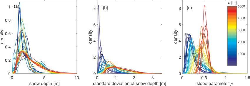
618 N. Helbig et al.: Fractional snow-covered area
Figure 2. Probability density functions for fine-scale (a) snow depth, (b) elevation and (c) squared-slope-related parameter per observation
data set in its original horizontal resolution, i.e., between 0.1 and 3 m. Densities were normalized with the corresponding maximum density of
all data sets. Note that for elevation (b) the y axis was cut for better visibility. Colors represent the different geographic regions, measurement
platforms or acquisition dates (number) of the compiled data set as indicated in Sect. 2.1 to 2.4.
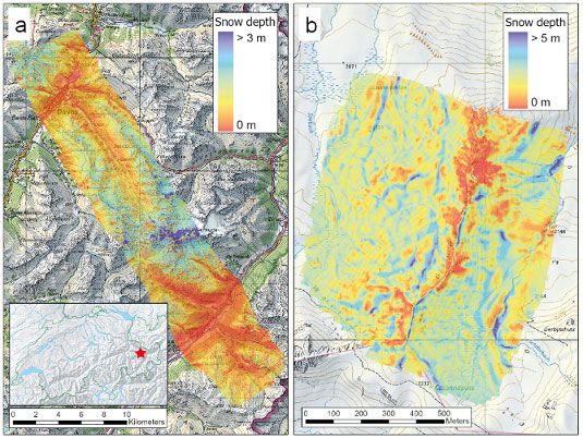
Figure 3. Snow depth maps of the eastern Swiss Alps: (a) in the Dischma region (ALS data) and (b) at Gaudergrat (UAS data) at the peak of
winter. The red dot in the inset map for Switzerland shows the location of the two sites. Pixmap © 2020 Swisstopo (5704000000), reproduced
with the permission of Swisstopo (JA100118).
were acquired from the Wannengrat and Dischma areas near dian absolute deviation (NMAD) of the residuals (Höhle and
Davos in the eastern Swiss Alps (Bühler et al., 2015). ADS- Höhle, 2009) of 26 cm.
derived snow depth data sets were used from 20 March The second platform was an unmanned aerial system
2012 (“ads-CH2 ”) to 9 March 2016 (“ads-CH1 ”), together (UAS) recording optical imagery with real-time kinematic
with summer digital elevation models (DEMs) (Marty et al., (RTK) positioning of the image acquisition points of the
2019). The data set covers about 150 km2 at 2 m resolution. snow cover with a standard camera over two different smaller
Bühler et al. (2015) validated the 2 m ADS-derived snow regions near Davos in the eastern Swiss Alps (Bühler et al.,
depth data among others with TLS data. They obtained a root 2016; Eberhard et al., 2021). These images were photogram-
mean square error (RMSE) of 33 cm and a normalized me- metrically processed into a digital surface model (DSM). By
subtracting the snow-free DSM from the winter flight, the
The Cryosphere, 15, 615–632, 2021 https://doi.org/10.5194/tc-15-615-2021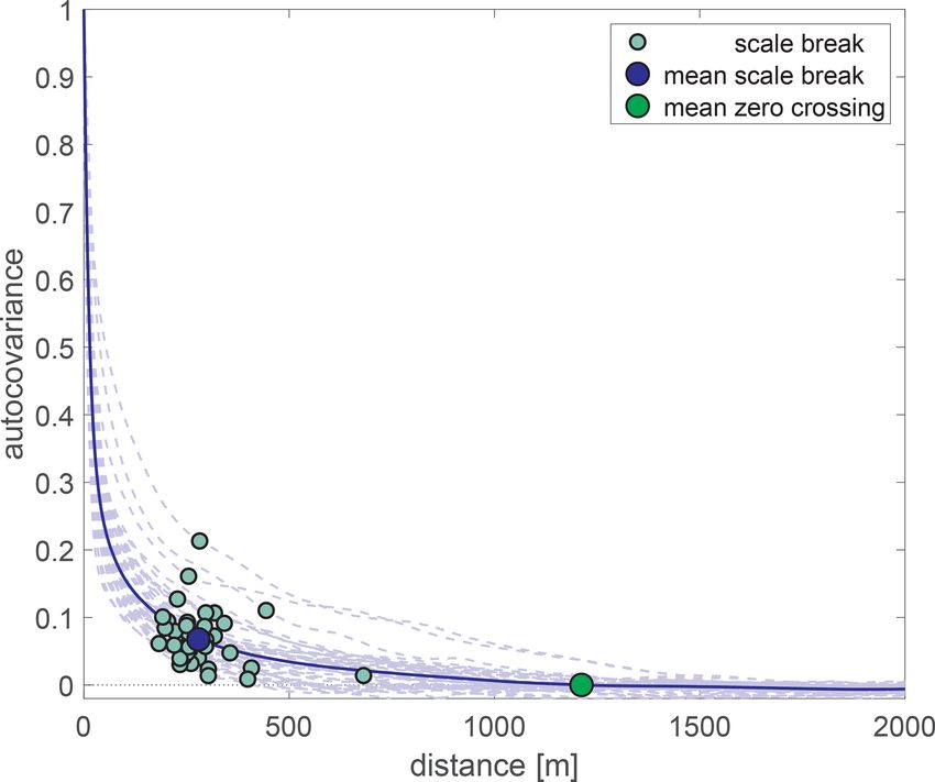
N. Helbig et al.: Fractional snow-covered area                                                                            619

HS values were obtained (Bühler et al., 2017). An UAS-          of 80 cm, a NMAD of 69 cm and a mean bias of 8 cm were
derived snow depth data set was used from 7 April 2018          obtained for the Pléiades data set.
(“uav-CH9 ”) from Schürlialp, together with a UAS-acquired
summer DEM (Eberhard et al., 2021). The Schürlialp data         2.3    Eastern French Pyrenees
set covers about 3.2 km2 which we used at 30 cm resolution.
A second UAS-derived snow depth data set was used from          A Pléiades product was acquired over the Bassiès basin in the
29 March 2019 (“uav-CH8 ”) from Gaudergrat, together with       northeastern French Pyrenees. Pléiades-derived snow depth
a UAS-acquired summer DEM. The Gaudergrat data set cov-         data were used from 15 March 2017 (“plei-FR4 ”), together
ers about 0.8 km2 at 10 cm resolution (Fig. 3b). Compared to    with a summer DEM (Marti et al., 2016). The data set we
snow depth data from snow probing, Eberhard et al. (2021)       used covers about 113 km2 at 3 m resolution. Marti et al.
obtained an RMSE of 16 cm and a NMAD of 11 cm for UAS-          (2016) derived a median of the bias between 2 m Pléiades
derived snow depth data at 9 cm horizontal resolution from      data and snow probe measurements of −16 cm and with UAS
Schürlialp.                                                     measurements of −14 cm. They further obtained a NMAD of
   The third platform was airborne laser scanning (ALS)         45 cm with snow probe measurements and a NMAD of 78 cm
above the Dischma region near Davos in the eastern Swiss        with UAS measurements.
Alps (Fig. 3a). This acquisition was a Swiss partner mis-
sion of the Airborne Snow Observatory (ASO) (Painter et al.,    2.4    Southeastern French Alps
2016). For consistency reasons, the same lidar setup was
used, and similar processing standards to the ASO campaigns     TLS-derived snow depth data were acquired at two alpine
in California were applied (Sect. 2.2). ALS-derived snow        mountain passes in the southeastern French Alps. One snow
depth data were used from 20 March 2017 (“als-CH3 ”), to-       depth data set was acquired over Col du Lac Blanc on
gether with a summer DEM from 2017. The ALS data set            9 March 2015 (“tls-FR10 ”) (Revuelto et al., 2020). A site and
from Switzerland used here covers about 260 km2 at 3 m res-     data description can be found in Naaim-Bouvet et al. (2010),
olution. Details on the derivation of the ALS data can be       Vionnet et al. (2014), and Schön et al. (2015, 2018). We used
found in Mazzotti et al. (2019), though this study focused on   a UAS-acquired summer DEM (Guyomarc’h et al., 2019).
three 0.5 km2 forested sub-data sets. Validation of 1 m ALS-    The data set covers about 0.6 km2 at 1 m resolution. The sec-
derived snow depth grids from 20 March 2017 against data        ond TLS-derived snow depth data set was acquired over Col
from snow probing within the forest but outside the canopy      du Lautaret at 27 March 2018 (“tls-FR5 ”) (Revuelto et al.,
(i.e., not below a tree) resulted in an RMSE of 13 cm and a     2020, ?). We used a TLS-acquired summer DEM. The data
bias of −5 cm.                                                  set covers about 0.14 km2 at 1 m resolution. Previously, mean
                                                                biases between 4 and 10 cm for TLS laser target distances
                                                                up to 500 m were obtained between TLS-derived and refer-
2.2   The Sierra Nevada, CA, US                                 ence tachymetry measurements (Prokop, 2008; Prokop et al.,
                                                                2008; Grünewald et al., 2010).
We used data sets acquired by two different platforms above
                                                                2.5    Preprocessing
Tuolumne basin in the Sierra Nevada (California) in the US.
   The first platform was ALS performed by ASO (Painter         In all data sets, grid cells 1x with forest, rivers, glaciers
et al., 2016). ALS-derived snow depth data were used from       or buildings were masked out. In order to avoid introducing
26 March 2016 (“als-US7 ”) and 2 May 2017 (“als-US6 ”),         any biases, we consistently neglected fine-scale snow depth
together with a summer DEM (Painter, 2018). The second          values in all data sets that were lower than 0 m or larger
platform was a Pléiades product from 1 May 2017 (“plei-         than 15 m. We used a snow depth threshold of 0 m to decide
US6 ”). A detailed data description of the Pléiades data set    whether or not a fine-scale grid cell was snow-covered.
derivation is given in Deschamps-Berger et al. (2020).
   We used the ASO summer DEM for the Pléiades, as well
as the ALS snow depth data sets. Given that the extent of       3     Methods
the Pléiades snow depth data set was much smaller than the
ALS domain, we cropped the ALS data sets to the Pléiades        We parameterize the standard deviation of snow depth σHS to
data set extension resulting in a coverage of about 280 km2 .   reassess the validity of the fSCA parameterization for com-
The horizontal resolution used here was 3 m for both data       plex topography from Helbig et al. (2015) for a range of spa-
sets. Compared to snow probe measurements in relatively         tial scales, in particular for sub-kilometer spatial scales.
flat areas, ALS snow depth data at 3 m horizontal resolution
was found unbiased with an RMSE of 8 cm (Painter et al.,        3.1    Fractional snow-covered area parameterization
2016). Pléiades-derived snow depth data were recently vali-
dated with ASO data over 137 km2 at 3 m resolution above        Helbig et al. (2015) derived an fSCA parameterization by
Tuolumne basin (Deschamps-Berger et al., 2020). An RMSE         integrating a normal pdf assuming spatially homogeneous

https://doi.org/10.5194/tc-15-615-2021                                                 The Cryosphere, 15, 615–632, 2021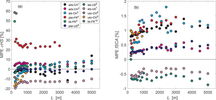
620                                                                              N. Helbig et al.: Fractional snow-covered area

melt. Subsequent fitting over a range of coefficients of vari-
ation CV (standard deviation divided by its mean) between
0.06 and 1.00 resulted in a similar closed form fit for fSCA
as Essery and Pomeroy (2004) obtained by integrating a log-
normal pdf,

                  HS
fSCA = tanh 1.3          ,                                (1)
                  σHS

using current HS and the standard deviation of previous max-
imum snow depth or peak of winter. The standard deviation
of snow depth at the peak of winter was derived by relating
the peak of winter high-resolution spatial snow depth data
from Switzerland and Spain to underlying summer terrain
parameters (Helbig et al., 2015):
                  h          i
σHS = HSa µb exp −(ξ/L)2 ,                               (2)
                                                                     Figure 4. Total number of valid domain sizes L per domain size L
                                                                     in log–log scale.
with a = 0.549, b = 0.309, HS and terrain correlation length
ξ are in meters, and ξ and µ are summer terrain parame-
ters, where µ is related to the mean squared slope via µ =
n                        o1/2                                        depth HS lower than 5 cm. By applying these limitations and
  [(∂x z)2 + (∂y z)2 ]/2      using partial derivatives of subgrid   since horizontal resolutions 1x, as well as the overall ex-
terrain elevations z, i.e., from a DEM. The correlation length       tent of the data sets, vary, the full range of L values, con-
ξ or typical width of topographic
                           √           features in a domain size     sisting of 41 different L values, was not represented by each
L was derived via ξ = 2σz /µ with the standard deviation             data set. Overall, this resulted in a pool of 367 643 domains
of elevations σz . The L/ξ ratio indicates how many charac-          with L values between 3 m and 5 km. We obtain a decreas-
teristic topographic features of length scale ξ are included         ing number of domains for increasing L with a range be-
in each L. Figure 2 in Helbig et al. (2009) shows a tran-            tween 59 376 for L = 90 m and 17 for L = 5000 m (Fig. 4).
sect of a topography indicating the described characteristic         Spatial averages and standard deviations were built for each
length scales. Similar to Helbig et al. (2015), we linearly de-      L. The resulting pooled data set shows a large variability in
trended the summer DEM before deriving the terrain param-            summer terrain characteristics. Spatial average slope angles
eters to unveil the correct terrain characteristics associated       range from 4 to 60◦ (µ from 0.05 to 1.22; Fig. 5c), terrain cor-
with the shaping process of the snow depth distribution at           relation lengths ξ from 6 to 775 m and L/ξ -ratios from 3 to
the corresponding scale. Using Eq. (1), fSCA can thus be             40. Thus, typical summer terrain characteristics captured by
derived with grid cell mean snow depth from a snow model             coarse climate model grid cells are well represented. The di-
and grid cell mean subgrid terrain parameters derived from a         versity of the remaining domains with regards to snow depth
fine-scale summer DEM. With the σHS formulation shown in             is shown by means of the pdfs for spatial mean HS and σHS
Eq. (2), Helbig et al. (2015) extended the fSCA parameteri-          as a function of domain size L in Fig. 5a and b. Since the data
zation (Eq. 1) for mountainous terrain.                              pool also covers a broad range in spatial mean HS (from 5 cm
                                                                     to 12.4 m) and spatial variability in snow depth σHS (from
3.2   Aggregating and pooling of data sets                           1 cm to 4.6 m) (Fig. 5a and b), we assume interannual snow
                                                                     depth variability is well described. In the following, overbars
Pooling all snow depth data sets yields a data pool with a vast      are neglected for spatial averages, i.e., for instance HS repre-
variety in snow climates, topographic characteristics and thus       sents spatial mean snow depth exclusively.
snow depth distributions. We first aggregated all snow data
in squared domain sizes L in regular grids between 3 m and           3.3   Autocovariances for scale breaks
5 km covering each geographic site. Our choice of the small-
est applicable L in a data set was defined by a large enough         The spatial autocovariance allows us to find spatial scale
L/1x ratio (here ≥ 20) to minimize the influence of grid cell        breaks up to which snow depth values are highly correlated,
resolutions when spatially averaging (Helbig et al., 2009).          i.e., up to which length scale the snow depth distribution
When aggregating, we required at least 70 % valid data in a          is strongly dictated by local topographic interactions of the
domain size which was the maximum threshold to obtain a              snow cover with wind, precipitation and radiation. Below this
sufficient number of domains for the largest domain sizes L          scale, break process models should ideally explicitly resolve
of 3 m to 5 km. In addition to that, we excluded L with spa-         these interactions to reliably describe the spatial snow depth
tial mean slope angles larger than 60◦ and spatial mean snow         distribution. Above this scale break, we assume that dom-

The Cryosphere, 15, 615–632, 2021                                                         https://doi.org/10.5194/tc-15-615-2021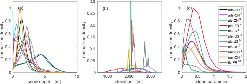
N. Helbig et al.: Fractional snow-covered area                                                                                         621

Figure 5. Probability density functions for (a) snow depth, (b) standard deviation of snow depth and (c) squared-slope-related parameter per
domain size L after preprocessing, pooling all data sets and building spatial averages.

inant wind or precipitation patterns due to larger-scale to-            i.e., domain size L. Based on the results of previous studies,
pography impacts dictate spatial snow depth distributions. At           we selected the following candidate parameters: HS, µ, sqS,
this scale range, the normalized standard deviations of snow            σsqS , L/ξ and σz .
depth σHS start leveling out (Fig. 6a), as well as the normal-
ized variability in σHS among similarly sized L (Fig. 6b).              3.5    Performance measures
   We calculated spatial autocovariances for snow depth data
sets with the fast Fourier transform (FFT), which allows for            The performance in this article is evaluated by the following
the computing of spatial autocovariances up to large dis-               measures: the root mean square error (RMSE), normalized
tances by keeping the fine grid cell resolutions. We used the           root mean square error (NRMSE; normalized by the range
R function fft() of the “stats” package (see R Core Team,               of measured data – max-min – or the mean of the measure-
2020). For each autocovariance, we then determine scale                 ments for fSCA), mean absolute error (MAE), the mean ab-
breaks using the R function uik() of the “inflection” package           solute percentage error (MAPE; absolute bias with measured
(R Core Team, 2020).                                                    minus parameterized and normalized with measurements),
                                                                        the mean percentage error (MPE; bias with measured minus
                                                                        parameterized and normalized with measurements) and the
3.4   Deriving a new scale-independent fractional
                                                                        Pearson correlation coefficient r as a measure for correla-
      snow-covered area parameterization
                                                                        tion. We also evaluate the performances by deriving the two-
                                                                        sample Kolmogorov–Smirnov test (K-S test) statistic values
Helbig et al. (2015) showed that fSCA performances in-                  D (Yakir, 2013) for the pdfs and by computing the NRMSE
creased with spatial scale and yielded their best performance           for quantile–quantile plots (NRMSEquant ; normalized by the
for spatial scales larger than 1000 m. Since the fSCA param-            range of measured quantiles, max-min) for probabilities with
eterization was empirically developed on snow depth data                values in the range of [0.1, 0.9].
from two geographic regions, here we reevaluated the scal-
ing variables for the spatial variability in snow depth σHS ,
as well as the functional form of the parameterization using            4     Results
the much larger compiled HS data set of this study. Various
scaling variables were previously employed to capture σHS               4.1    Spatial correlation range from snow depth data
in mountainous terrain. Helbig et al. (2015) selected HS, the
squared-slope-related parameter µ and the L/ξ ratio (Eq. 2).            We derived a total of 40 autocovariances for the available do-
Skaugen and Melvold (2019) used HS and the standard de-                 main sizes L of 3 km with grid cell sizes 1x of 2 or 3 m.
viation of the squared slope, with sqS being derived using              We obtained scale breaks between 183 and 681 m with a
sqS = tan2 ζ , where ζ is the slope angle in radians. Since             mean of 284 m (±σ 86 m) (Fig. 7). The zero crossings for
tan2 ζ is the same as 2µ2 (e.g., Löwe and Helbig, 2012), we             each autocovariance were between 402 and 1815 m with a
here derive sqS from 2µ2 . Several other studies used σz as             mean of 1011 m (±σ 402 m). For the mean autocovariance,
terrain parameter (e.g., Roesch et al., 2001). Here, we were            we obtained a scale break at about 279 m and a zero cross-
interested in finding dominant scaling variables that corre-            ing at about 1212 m. Based on the observed scale breaks,
late consistently across scales with σHS . We therefore ana-            we selected a minimum length scale of 200 m for deriving
lyzed the Pearson correlation coefficient r between various             a new scale-dependent fSCA parameterization for all larger
candidate parameters and σHS as a function of spatial scale,            scales. In the following, all results are therefore restricted to

https://doi.org/10.5194/tc-15-615-2021                                                            The Cryosphere, 15, 615–632, 2021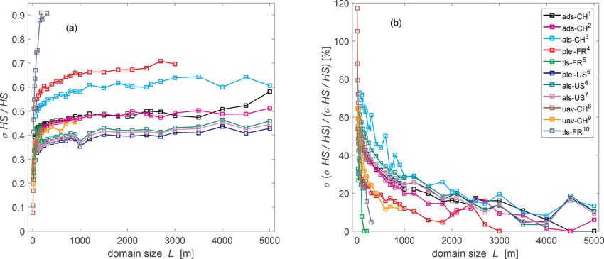
622                                                                                  N. Helbig et al.: Fractional snow-covered area

Figure 6. (a) Normalized standard deviation of HS as a function of domain size L for each data set separately. (b) Normalized percentage of
standard deviation of panel (a) among each L. L ranges from 3 m to 5 km. Colors represent the different geographic regions, measurement
platforms or acquisition dates (number) of the compiled data set as indicated in Sect. 2.1 to 2.4.

                                                                        correlation coefficients across scales but slightly smaller for
                                                                        L ≤ 1800 m resulted in the squared slope sqS having an over-
                                                                        all mean of 0.33. The correlation coefficients for the stan-
                                                                        dard deviation of sqS (σsqS ) and σz were much less consis-
                                                                        tent across scales than for µ and sqS and were overall lower.
                                                                        The mean correlation for σsqS is 0.15, for L/ξ 0.21 and for
                                                                        σz 0.01. Though the mean correlation between σHS and L/ξ
                                                                        is rather low, the correlation remains more consistent across
                                                                        scales up to about 2500 m and increases for larger scales con-
                                                                        siderably up to 0.67 (cf. Fig. 8a).
                                                                           We selected HS, µ and L/ξ as main scaling parameters for
                                                                        σHS across spatial scales from 200 m to 5 km (Fig. 8b).

                                                                        4.3   Scale-independent fSCA parameterization

                                                                        The correlation analysis across scales revealed the same
Figure 7. FFT-derived autocovariances for spatial snow depth. Indi-     dominant correlation parameters as in Helbig et al. (2015).
vidual ranges, mean range and mean autocovariance zero crossing
                                                                        We therefore kept the functional form for σHS at the peak
are shown.
                                                                        of winter suggested by Helbig et al. (2015) using the three
                                                                        scaling variables HS, µ and L/ξ . The new σHS parameter-
L ≥ 200 m, leaving a pool of 41 249 domain sizes L with L               ization at the peak of winter thus has the same functional
between 200 m and 5 km for the development of the parame-               form than the one suggested by Helbig et al. (2015) which
terization.                                                             was presented in Eq. (2). However, the fit parameters a and b
                                                                        therein are replaced by the new parameters c and d which we
4.2   Scaling variables for σHS                                         specify below. To derive the new parameters c, d, we fitted
                                                                        nonlinear regression models by robust M-estimators using it-
Correlation coefficients varied differently across spatial              erated reweighed least squares; see R (R Core Team, 2020)
scales (Fig. 8a). For all scales, we obtained the largest cor-          and its robustbase package version 0.93-6 (Maechler et al.,
relation coefficients for HS ranging from 0.48 to 0.98 with             2020). We started at the scale length of 200 m, defined by the
a mean of 0.79. From correlations with the various subgrid              scale break which we derived before from spatial snow depth
terrain parameters, the largest correlations across all scales          autocovariances.
were reached for the squared-slope-related parameter µ rang-               Fit parameters were first derived for the entire data pool
ing from 0.22 to 0.61 with a mean of 0.36. Similar consistent           and L ≥200 m yielding c = 0.6589 (±0.0037) and d =

The Cryosphere, 15, 615–632, 2021                                                             https://doi.org/10.5194/tc-15-615-2021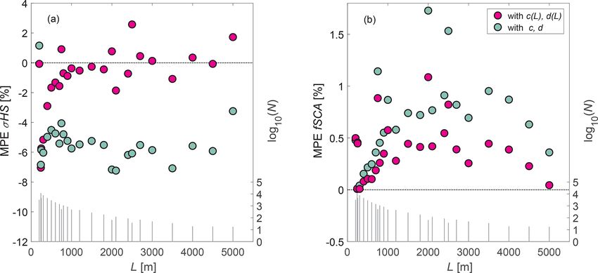
N. Helbig et al.: Fractional snow-covered area                                                                                       623

Figure 8. (a) Correlation coefficients between σHS and various parameters as a function of domain size L. (b) Standard deviation of snow
depth σHS as a function of HS and µ.

                                                                           (cf. Fig. 4). Thereby, each sub-data pool comprised all do-
                                                                           mains larger than or equal to the corresponding domain size,
                                                                           i.e., L ≥ 200 m, L ≥ 240 m, etc. Fitting over such a sub-data
                                                                           pool should allow us to describe the combined larger-scale
                                                                           topography–wind–precipitation impacts on the spatial snow
                                                                           depth distribution in mountainous terrain acting at scales
                                                                           larger than the observed scale break of about 200 m. From
                                                                           each of the 25 created sub-data pools, we randomly took 500
                                                                           subsamples in which each subsample was restricted to 80 %
                                                                           data of the sub-data pool. Each of the 500 subsamples per
                                                                           sub-data pool was unique. Scale-dependent parameter val-
                                                                           ues were derived for each of the 500 subsamples drawn from
                                                                           each of the 25 sub-data pools (cf. individual colored lines in
                                                                           Fig. 9). Given that the values of c, d clearly increase with
                                                                           spatial scale L (Fig. 9), we introduced L in c, d to improve
                                                                           the application of Eq. (2) across scales. By fitting the en-
Figure 9. Fit parameters for Eq. (2) as a function of domain sizes L       semble medians of all scale-dependent fit parameters (dark
to scale variables (a) HS and (b) µ. Colored lines show the fit pa-        blue dots in Fig. 9) across all domain sizes between 200 m
rameters derived for each of the 500 random 80 % samples of each           and 5 km, we obtained scale-dependent parameters c(L) and
of the 25 sub-data pools. The dark blue dots depict the ensemble           d(L). Thus, Eq. (2) using the following scale-dependent pa-
median per L. Previously obtained constant parameters of Helbig            rameters c(L) and d(L) assembles our new σHS parameteri-
et al. (2015) (light blue dots) and newly fitted constant (red dots), as   zation for L ≥ 200 m:
well as newly fitted scale-dependent (pink circles) parameters are
shown.                                                                     c(L) = 0.5330L0.0389 ,
                                                                           d(L) = 0.3193L0.1034 ,                                     (3)

0.5638 (±0.0043) with the 90 % confidence intervals of the                 with the 90 % confidence intervals of ±0.0097, ±0.0026 and
fit parameters given in parentheses. These “new” constant pa-              ±0.0183, and ±0.0079 in the order of introduced constants
rameters c, d are larger than the previously derived constants             in Eq. (3).
a, b in Eq. (2) (cf. Fig. 9).                                                 The new σHS parameterization using c(L) and d(L) (Eq. 2
    In addition to fitting over the entire data pool and                   with Eq. 3) is applied in the previously derived fSCA param-
L ≥ 200 m, we split the entire data pool into 25 sub-data                  eterization (Eq. 1). To demonstrate the resulting differences
pools for any available domain size between 200 m and 5 km                 when using scale-dependent versus scale-independent fit pa-

https://doi.org/10.5194/tc-15-615-2021                                                              The Cryosphere, 15, 615–632, 2021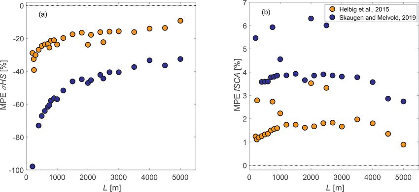
624                                                                            N. Helbig et al.: Fractional snow-covered area

rameters in parameterized σHS (Eq. 2), we will also validate      hand do not show a similar large spread among the regions
the performance using constant c, d in the previously derived     and are low between −1 % to 2 % (Fig. 11b).
fSCA parameterization, as well as in the σHS parameteriza-
tion.                                                             4.4.4    Evaluation of previous closed form
                                                                           parameterizations
4.4     Evaluation
                                                                  To increase our understanding of the performances achieved
4.4.1    Evaluation for σHS and fSCA for all L values             with the new parameterizations, we also tested two previ-
                                                                  ously derived empirical parameterizations. Specifically, we
Parameterized σHS and fSCA perform well for all domain            investigated how parameterized σHS using Eq. (2) (Helbig
sizes, i.e., for L ≥ 200 m, of the entire data pool. Very simi-   et al., 2015) and using the recently published formulation
lar performance measures are obtained for the parameteriza-       of Skaugen and Melvold (2019) compare to observed σHS
tions using the newly derived constant fit parameters c, d and    of our compiled data set (Fig. 12a). We further tested both
the parameterizations using the scale-dependent parameters        σHS parameterizations in the fSCA parameterization (Eq. 1;
c(L), d(L) (cf. Table 1 and Ia and IIa). We obtain a slightly     Fig. 12b). The parameterization of Helbig et al. (2015) works
better MPE for σHS when using scale-dependent fit parame-         well. The performance measures for all L values are only
ters (−4 % versus -5 %); however, for fSCA, MPEs are the          slightly worse compared to the new parameterizations us-
same (0.2 %). The same rather low NRMSE results for σHS           ing both constant and scale-dependent fit parameters (Ta-
(8 %) and for fSCA (2 %) are obtained when using constant         ble 1). However, compared to the performance measures for
or scale-dependent fit parameters.                                the parameterization of Skaugen and Melvold (2019), the
                                                                  performances of Helbig et al. (2015) are clearly improved.
4.4.2    Scale-dependent evaluation for σHS and fSCA              Though MPEs of both previous σHS parameterizations are
                                                                  scale-dependent, the MPEs of Skaugen and Melvold (2019)
While mean performance measures of the σHS and fSCA pa-           reveal a larger scale-dependency of the performances com-
rameterization are almost uninfluenced by using constant or       pared to Helbig et al. (2015) (Fig. 12a). In particular, indi-
scale-dependent fit parameters (cf. Table 1 and Ia and IIa), we   vidual MPEs vary a lot from MPEs for all L values given in
found diverging performances when analyzing performance           Table 1.
measures as a function of scale (Fig. 10). Across scales,
improved or similar performances were achieved when us-
ing scale-dependent fit parameters in parameterized σHS , es-     5     Discussion
pecially for larger scales. Maximum performance improve-
ments for σHS of 4 % and for fSCA of 0.7 % occurred for L         5.1     Spatial correlation range
of 2500 m when using scale-dependent fit parameters. Thus,
introducing scale-dependent fit parameters enhanced the σHS       While multiscale behavior for spatial snow depth data has
parameterization for application across scales.                   been found in various studies, observed scale breaks depend
                                                                  on the extent and horizontal resolution of the investigated
4.4.3    Scale- and region-dependent evaluation for σHS           snow depth data sets. A first scale break of spatial snow
         and fSCA                                                 depth data in treeless, alpine terrain has been observed be-
                                                                  tween 10 to 20 m (e.g., Deems et al., 2006; Trujillo et al.,
A large data set from various geographic regions allows us        2007; Schweizer et al., 2008; Schirmer and Lehning, 2011;
to develop a more reliable empirical parameterization than        Helfricht et al., 2014; Mendoza et al., 2020), and a second
being limited to the characteristics of a few data sets. Here,    scale break has been observed at around 60 m (Trujillo et al.,
we not only compiled data sets from various geographic re-        2009). By computing spatial autocovariances starting with
gions, but the data sets were also acquired by different mea-     domain sizes L of 200 m at 0.1 to 1 m resolution and increas-
surement platforms coming with a range of inaccuracies be-        ing up to 3 km at 2 to 3 m resolution, we also detected the
tween below 10 and 80 cm. As a consequence, larger scat-          two previously found scale breaks (not shown). However, by
ter in performances appears when performance measures are         additionally covering larger spatial extents than have been
depicted not only as a function of spatial scale but also re-     previously investigated, we also detected a third scale break
gionwise, including platformwise. While most of the MPEs          with a mean at about 280 m (Fig. 7). Similar long-range scale
are still between −20 % and 10 %, some regions stand out          breaks between 185 and 300 m were very recently reported
because they have much larger MPEs when binned by scale,          from analyzing 24 TLS-derived snow depth data sets ac-
as well as by region (Fig. 11). For instance, a MPE of up         quired during six snow seasons in a subalpine catchment in
to 60 % for σHS was obtained for TLS data from the south-         the Spanish Pyrenees (Mendoza et al., 2020). Furthermore,
eastern French Alps, and overall larger MPEs, though consis-      a similar scale break at around 200 m was recently found by
tent across scales, for the Pléiades data from the northeastern   analyzing performance decreases in distributed snow model-
French Pyrenees were obtained. MPEs for fSCA on the other         ing in various grid cell sizes, together with a semivariogram

The Cryosphere, 15, 615–632, 2021                                                      https://doi.org/10.5194/tc-15-615-2021
N. Helbig et al.: Fractional snow-covered area 625
Table 1. Performance measures for all L values between measurement and parameterization of (I) standard deviation of snow depth σHS
with (a) Eq. (2) and constant or L-dependent fit parameters c, d (Eq. 3) and (b) σHS as in Helbig et al. (2015) and Skaugen and Melvold
(2019) and of (II) fSCA with (a) Eq. (1) and (1a) and (b) fSCA as in Helbig et al. (2015) and Skaugen and Melvold (2019) using Eq. (1).
NRMSE RMSE MPE MAPE MAE r K-S NRMSEquant
(%) (cm) (%) (%) (cm) (%)
(I) σHS
(a) Eq. (2) with
constant c, d parameter 7.9 26.6 −5.3 22.6 19.7 0.83 0.05 5.3
c(L), d(L) (Eq. (3)) 7.9 26.7 −4.1 22.4 19.6 0.83 0.05 5.5
(b) Previous parameterizations from
Helbig et al. (2015) 9.3 31.1 −29.5 36.7 25.3 0.82 0.22 14.6
Skaugen and Melvold (2019) 20.4 68.5 −77.9 82.8 57.9 0.68 0.48 37.6
NRMSE RMSE MPE MAPE MAE r K-S NRMSEquant
(%) (%) (%) (%)
(II) fSCA
(a) Eq. (1) with
Eq. (2) and constant c, d parameter 2.4 0.02 0.22 1.11 0.01 0.64 0.37 0.5
Eq. (2) and c(L), d(L) (Eq. 3) 2.4 0.02 0.16 1.09 0.01 0.63 0.37 0.4
(b) Previous parameterizations from
Helbig et al. (2015) 3.2 0.03 1.45 1.8 0.02 0.74 0.47 1.6
Skaugen and Melvold (2019) using Eq. (1) 6.2 0.06 3.87 4.8 0.05 −0.04 0.75 4.4
Figure 10. Mean percentage error (MPE) as a function of L for (a) σHS and (b) fSCA. MPEs are shown for the σHS and fSCA parameteriza-
tions using Eq. (1) to (3) with scale-dependent c(L), d(L), as well as for constant c, d. The second y axis shows the number of valid domains
per L on a logarithmic scale.
analysis of subgrid summer terrain slope angles in the same influence the spatial snow distribution in mountainous ter-
catchment in the High Atlas (Baba et al., 2019). While for rain, while we believe there are different physical processes
other application studies, such as in avalanche forecasting, which establish the smaller-scale breaks at around 10 to 20
the smaller-scale breaks are decisive for explicitly describing and 60 m. The results presented here indicate that the model
the relevant snow-cover processes, here we are more inter- described by Eqs. (1) and (3) is reliably parameterizing the
ested in the largest detected scale break. Above scale lengths spatial snow distribution shaped by the longer-range precip-
of 200 m, the longer-range processes of precipitation, wind itation, wind and radiation interactions with topography for
and radiation interactions with topography most dominantly spatial scales between 200 m and 5 km. Above the detected
https://doi.org/10.5194/tc-15-615-2021 The Cryosphere, 15, 615–632, 2021626 N. Helbig et al.: Fractional snow-covered area
Figure 11. Mean percentage error (MPE) as a function of L for the compiled data set for (a) σHS and (b) fSCA using Eqs. (1) to (3) with
scale-dependent c(L), d(L). Colors represent the different geographic regions, measurement platforms or acquisition dates (number) of the
compiled data set as indicated in Sect. 2.1 to 2.4.
Figure 12. Mean percentage error (MPE) as a function of L for the compiled data set for (a) σHS and (b) fSCA. MPEs are shown for the
σHS and fSCA parameterizations of Helbig et al. (2015), as well as for the σHS parameterization of Skaugen and Melvold (2019) and the
σHS parameterization of Skaugen and Melvold (2019) applied in the fSCA parameterization of Helbig et al. (2015) (Eq. 1).
scale range of around 200 m, not only the spatial autocorre- tial scale. For some commonly applied scaling parameters,
lations approach zero (Fig. 7), but normalized σHS clearly this revealed large variations in correlations across scales
start leveling out, as well as the normalized variability in such as for σz (Fig. 8a). Similar to our results, Skaugen
σHS among similarly sized L (Fig. 6). Thus, even though we and Melvold (2019) also obtained large correlations between
could not verify the fSCA parameterization for length scales σHS and mean squared slope sqS for spatial snow depth data
larger than 5 km, we believe that as long as grid cell mean sets acquired at the peak of winter in Norway, though this
slope angles are larger than zero, Eqs. (1) and (3) might also was only analyzed for grid cells of 0.5 km2 (0.5 km × 1 km).
hold for larger grid cell sizes than 5 km. Nevertheless, this confirms our findings since mean squared
slope is related to the slope-related parameter µ used here
5.2 Scaling parameter by sqS = 2µ2 . However, Skaugen and Melvold (2019) ob-
tained a slightly improved correlation for the standard devia-
We not only investigated dominant correlations between the tion of squared slope and therefore selected this parameter to
spatial snow depth distribution and terrain parameters, but stratify the topography for parameterizing σHS . Across spa-
we also analyzed these correlations as a function of spa-
The Cryosphere, 15, 615–632, 2021 https://doi.org/10.5194/tc-15-615-2021N. Helbig et al.: Fractional snow-covered area 627
tial scales, as well as for all L values, we obtained lower performance), we obtained very similar performances when
correlations between the standard deviation of squared slope using newly derived constant or scale-dependent fit parame-
and σHS , though we observed cross-correlations between the ters, i.e., c, d or c(L), d(L) (Table 1). Despite considerable
mean and the standard deviation of squared slope of 0.71, differences up to 12 % for c and up to 38 % for d between
indicating that both parameters correlate well with σHS . constant and scale-dependent fit parameters (Fig. 9), pooled
performances for all L values for σHS and fSCA were sim-
5.3 Scale-independent fSCA parameterization ilar (Table 1). An explanation for this is that the number of
available domains is strongly decreasing with increasing L.
The closed form fractional snow-covered area parameteriza- For L ≥ 3000 m, we have only about 0.33 % (137 in total)
tion fSCA given in Eq. (1) got enhanced by recalibration and valid domains available compared to the total of 41 249 for
introducing scale-dependent fit parameters (Eq. 3) to make L < 3000 m (Fig. 4). This emphasizes the need for a scale-
the performance consistent across spatial scales. dependent evaluation.
We developed the parameterization on a large snow depth
data set. Large variability in the snow depth data set was 5.4.2 Scale-dependent evaluation for σHS and fSCA
gained by compiling 11 individual data sets from varying ge-
ographic regions, as well as various measurement platforms. The largest improvement in MPE for all L values seems to
While the latter might explain the remaining performance originate from the recalibration using the new compiled data
differences discussed below, the first led to large variabil- set with a reduction in MPE from −30 % to −5 % com-
ity in summer terrain characteristics and snow climates and pared to a reduction from −5 % to −4 % when introducing
consequently spatial snow depth distributions (cf. Fig. 2). scale-dependent fit parameters (Table 1). However, MPEs as
Though our presented parameterization for σHS was empiri- a function of scale clearly demonstrated the improved behav-
cally derived, it is reassuring that for a new empirical deriva- ior when using scale-dependent c(L), d(L) instead of con-
tion on a much larger and more diverse snow depth data stant fit parameters c, d in the σHS and fSCA parameteriza-
set, the same underlying functional form could be used. Fur- tion (Fig. 10). Given that constant c, d were fitted over the
thermore, larger (about 17 % and 45 %) but overall consis- entire data set as have been c(L), d(L), any performance im-
tent constant fit parameters were obtained compared to those provement using c(L), d(L) instead of constant c, d for pa-
from Helbig et al. (2015) based on a more limited number of rameterized σHS and fSCA originates in introducing scale-
data sets and just two geographic regions (cf. a and b in Eq. 2 dependent parameters. For the parameterizations using the
and c, d presented in Sect. 4.3 or Fig. 9). constant fit parameters c, d, errors varied slightly more across
In addition to deriving constant fit parameters across spa- scales than when using the scale-dependent c(L), d(L) ver-
tial scales, we took 500 random 80 % subsamples from sion. Individual scale-dependent errors were in part larger
each of the 25 sub-data pools (Sect. 4.3). Scale-dependent than the MPEs for all L values given in Table 1. Unequal
constants considerably increased with increasing scale from numbers of valid domains per L most likely also contributed
L = 200 m to L = 5 km by at most 12 % and 38 %, respec- to this.
tively (Fig. 9). This demonstrates that accounting for scale-
dependent constants in the fSCA parameterization (Eq. 1 5.4.3 Scale- and region-dependent evaluation for σHS
with Eqs. 2 and 3) had to be done. While we did not split and fSCA
our data set in development and validation subsets, fitting
over the ensemble median of all scale-dependent parameters While we did not perform an evaluation using independent
to derive c(L), d(L) ensures confidence in the resulting fit snow depth data sets, studying regionwise performances re-
parameters. veals the spread in errors we can expect when the new param-
An increase in scatter among all c(L) and d(L) with in- eterizations are applied on an individual independent data
creasing domain scale L (Fig. 9) can be most likely explained set (Fig. 11). We obtain much larger positive MPEs for σHS
by a concurrent decrease in available valid data in larger L at lower spatial scales of L = 200 m and L = 300 m for the
values. Though we required at least 70 % valid data per L two TLS data sets in the southeastern French Alps and over-
when aggregating fine-scale snow depth data in domain sizes all larger MPEs between 20 % and 30 %, though consistent
L, the maximum threshold of 70 % was more often required across scales, for the Pléiades data from the Bassiès basin in
for the larger L values than for smaller L values. the northeastern French Pyrenees. It is unclear if these larger
MPEs originate in uncertainties of the data acquisition, i.e.,
5.4 Evaluation are platform specific, or if they are linked to spatial snow
depth distributions which could not be captured by the pro-
5.4.1 Evaluation for σHS and fSCA posed new parameterizations. RMSEs for the various remote
sensing platforms and data sets used here (Sect. 2) decrease
Upon deriving performance measures on parameterized and from 80 cm for Pléiades data from the Sierra Nevada to 33 cm
observed σHS and fSCA for all L values (i.e., the pooled for the ADS, to 16 cm for UAS, to 13 cm for ALS data from
https://doi.org/10.5194/tc-15-615-2021 The Cryosphere, 15, 615–632, 2021628 N. Helbig et al.: Fractional snow-covered area
Switzerland, to 8 cm for ALS data from the Sierra Nevada 6 Conclusions
and to 4 to 10 cm for TLS data in general. Given the rather
low errors typically obtained for TLS data compared to the We presented an empirical peak of winter parameterization
other remote sensing platforms, the reason for the large de- for the standard deviation of snow depth σHS for treeless,
viations in the TLS data sets might not originate in inaccu- mountainous terrain, describing the spatial snow depth distri-
racies of the data acquisition. On the contrary, the observed bution in a grid cell for various model applications. The scal-
bias in the Pléiades data from the northeastern French Pyre- ing variables in the new parameterization of σHS and fSCA
nees might indeed be attributed to the rather large inaccu- are the same as in Helbig et al. (2015) which are spatial mean
racies of the platform with NMADs of 45 to 78 cm (Marti snow depth, a squared-slope-related parameter and a terrain
et al., 2016). However, Pléiades data from the Sierra Nevada correlation length. All subgrid terrain parameters can be eas-
come with a similarly large NMAD of 69 cm, but σHS can be ily derived from fine-scale summer DEMs for each coarse
parameterized very well with MPEs lower than ±3 % across grid cell.
spatial scales (Fig. 11a). Observed σHS from the TLS, as well By introducing spatial scale dependencies in the variables
as from the Pléiades data in France, was considerably larger in the formulation for σHS of Helbig et al. (2015), σHS can
than parameterized σHS , but mean slope angles alone can also be consistently parameterized across spatial scales starting at
not explain this behavior (between 6 and 23◦ for the TLS data scales ≥200 m. The spatial snow depth variability or σHS is
and between 13 and 50◦ for the Pléiades data). the important variable to parameterize the fractional snow-
While we were not able to clearly relate some of the covered area or fSCA (Helbig et al., 2015). Performance im-
poorer regionwise performances to uncertainties related to provements across spatial scales of the σHS parameterization
the platform, other studies entirely focused on perform- therefore directly enhanced the fSCA parameterization. Be-
ing extensive intercomparisons between platforms for large- tween length scales of 200 m and 5 km, mean percentage er-
scale snow depth mapping in alpine terrain (e.g., Bühler rors (MPE) were between −7 % and 3 % for σHS and between
et al., 2015, 2016; Eberhard et al., 2021; Deschamps-Berger 0 % and 1 % for fSCA.
et al., 2020). The subgrid parameterization of σHS was developed from
11 spatial snow depth data sets from seven different geo-
5.4.4 Evaluation of previous closed form graphic regions at high spatial resolutions between 0.1 to
parameterizations 3 m and with spatial coverage between 0.14 to 280 km2 . An
evaluation of two previously presented empirical σHS pa-
Though we developed a new σHS parameterization (Eq. 3), rameterizations confirmed the functional form of the param-
empirically derived parameterizations can only describe the eterization of Helbig et al. (2015), as well as the need to
variability inherent in the data set used to derive the param- enhance its performance across scales. By analyzing data
eterization. In addition to the regionwise evaluation, analyz- from the large pool of spatial snow depth data sets, we were
ing performances of previous empirically derived parameter- able to recalibrate the subgrid parameterization of σHS and
izations may therefore allow us to estimate expected perfor- achieve improved performances using new constant fit pa-
mance sensitivity to independent data sets. While both tested rameters. Additionally introducing a scale dependency in the
parameterizations of σHS (Helbig et al., 2015; Skaugen and dominant scaling variables further improved the performance
Melvold, 2019) showed a worse performance than the new across spatial scales. Mean MPEs of σHS over all scales (i.e.,
parameterizations and less consistency as a function of scale, pooled performance) reduced from −30 % using Helbig et al.
the model performances of Helbig et al. (2015) were only (2015) to −5 % after recalibration to −4 % after introducing
slightly worse than the new parameterizations (Table 1). The scale-dependent fit parameters (Table 1). Individual scale-
parameterization for σHS of Skaugen and Melvold (2019) dependent improvements in MPEs reached up to 4 % when
was developed on mean domain sizes L of 750 m, whereas using newly derived scale-dependent fit parameters com-
Helbig et al. (2015) used L values between 50 m to 3 km. pared to newly derived constant fit parameters for σHS from
This difference might be one reason for the overall poorer the large data pool. This shows the improvement thanks to
performances of Skaugen and Melvold (2019) compared to introducing scale-dependent parameters (Fig. 10). Towards
Helbig et al. (2015) across spatial scales. Since only 1 out estimating the possible spread in performances when apply-
of the 11 data sets used in this study was previously used to ing empirically derived σHS and fSCA for independent ge-
develop the parameterization of Helbig et al. (2015), an over- ographic regions, we validated the parameterizations sepa-
all similar performance of Helbig et al. (2015) (Fig. 12) with rately for each region and scale. While this clearly increased
the large compiled data set of this study clearly confirms the MPEs for three data sets, the majority of the region- and
underlying functional form of σHS suggested by Helbig et al. scale-dependent MPEs were between ±10 % for σHS and be-
(2015) which was reapplied here. tween −1 % and 1.5 % for fSCA, indicating that the param-
eterizations perform similarly well in most geographical re-
gions.
The Cryosphere, 15, 615–632, 2021 https://doi.org/10.5194/tc-15-615-2021You can also read