The impact of secondary ice production on Arctic stratocumulus - Atmos. Chem. Phys
←
→
Page content transcription
If your browser does not render page correctly, please read the page content below
Atmos. Chem. Phys., 20, 1301–1316, 2020
https://doi.org/10.5194/acp-20-1301-2020
© Author(s) 2020. This work is distributed under
the Creative Commons Attribution 4.0 License.

The impact of secondary ice production on Arctic stratocumulus
Georgia Sotiropoulou1 , Sylvia Sullivan2 , Julien Savre3 , Gary Lloyd4 , Thomas Lachlan-Cope5 , Annica M. L. Ekman6 ,
and Athanasios Nenes1,7
1 Laboratory   of Atmospheric Processes and their Impacts, School of Architecture, Civil & Environmental Engineering,
École Polytechnique Fédérale de Lausanne (EPFL), Lausanne 1015, Switzerland
2 Department of Earth and Environmental Engineering, Columbia University, New York 10027, USA
3 Meteorological Institute, Faculty of Physics, Ludwig-Maximilians-Universität, Munich, Germany
4 Centre for Atmospheric Science, University of Manchester, Manchester, M139P, UK
5 British Antarctic Survey, Cambridge, CB3 0ET, UK
6 Department of Meteorology, Bolin Centre for Climate Research, Stockholm University, Stockholm, 11419, Sweden
7 Institute of Chemical Engineering Sciences, Foundation for Research & Technology – Hellas, Patras 26504, Greece

Correspondence: Georgia Sotiropoulou (georgia.sotiropoulou@epfl.ch) and Athanasios Nenes (athanasios.nenes@epfl.ch)

Received: 6 September 2019 – Discussion started: 17 September 2019
Revised: 16 December 2019 – Accepted: 10 January 2020 – Published: 4 February 2020

Abstract. In situ measurements of Arctic clouds frequently       1   Introduction
show that ice crystal number concentrations (ICNCs) are
much higher than the number of available ice-nucleating
particles (INPs), suggesting that secondary ice production       Mixed-phase clouds are a critical component of the Arc-
(SIP) may be active. Here we use a Lagrangian parcel model       tic climate system due to their warming effect on the sur-
(LPM) and a large-eddy simulation (LES) to investigate the       face radiation balance (Shupe and Intrieri, 2004; Sedlar et
impact of three SIP mechanisms (rime splintering, break-         al., 2011) and potential impact on the melting of sea ice.
up from ice–ice collisions and drop shattering) on a sum-        These clouds are very frequent in the summer, when they
mer Arctic stratocumulus case observed during the Aerosol-       occur about 80 %–90 % of the time and can persist for days
Cloud Coupling And Climate Interactions in the Arctic (AC-       to weeks (e.g., Shupe et al., 2011). However, their represen-
CACIA) campaign. Primary ice alone cannot explain the ob-        tation in mesoscale and large-scale numerical weather pre-
served ICNCs, and drop shattering is ineffective in the ex-      diction and climate models remains elusive (Karlsson and
amined conditions. Only the combination of both rime splin-      Svensson, 2013; Barton et al., 2014; Wesslén et al., 2014;
tering (RS) and collisional break-up (BR) can explain the        Sotiropoulou et al., 2016).
observed ICNCs, since both of these mechanisms are weak             An accurate description of mixed-phase clouds in models
when activated alone. In contrast to RS, BR is currently not     requires a solid knowledge of the amount and distribution of
represented in large-scale models; however our results indi-     both liquid water and ice (e.g., Korolev et al., 2017). Ice crys-
cate that this may also be a critical ice-multiplication mech-   tals and liquid drops form upon preexisting aerosols, termed
anism. In general, low sensitivity of the ICNCs to the as-       ice nucleating particles (INPs) and cloud condensation nuclei
sumed INP, to the cloud condensation nuclei (CCN) condi-         (CCN), respectively. However, the observed ice crystal num-
tions and also to the choice of BR parameterization is found.    ber concentration (ICNC) can be orders of magnitude higher
Finally, we show that a simplified treatment of SIP, using a     than the number of INPs (e.g., Rangno and Hobbs, 2001;
LPM constrained by a LES and/or observations, provides a         Gayet et al., 2009; Schwarzenboeck et al., 2009; Lloyd et
realistic yet computationally efficient way to study SIP ef-     al., 2015). The enhanced ICNCs are especially surprising in
fects on clouds. This method can eventually serve as a way       the high Arctic, which is relatively clean, with sparse INPs
to parameterize SIP processes in large-scale models.             (Morrison et al., 2012). Secondary ice production (SIP) is
                                                                 suggested as the cause to explain this cloud ice paradox (e.g.,
                                                                 Gayet et al., 2009; Lloyd et al., 2015). SIP refers to a variety

Published by Copernicus Publications on behalf of the European Geosciences Union.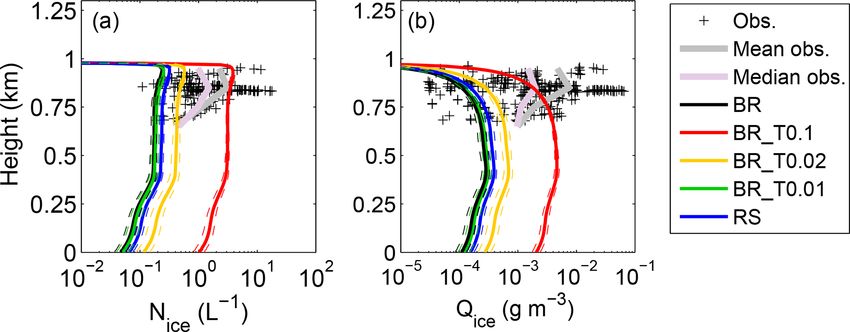
1302                               G. Sotiropoulou et al.: The impact of secondary ice production on Arctic stratocumulus

of collision-based processes that multiply the concentration        Arctic (ACCACIA) flight campaign in 2013. Observations of
of ice crystals in the absence of additional INPs (e.g., Field et   stratocumulus clouds from the summer flights indicate that
al., 2017, and references therein). However these processes         ICNCs were orders of magnitude higher than the measured
are poorly represented in atmospheric models, resulting in          aerosol concentrations that can act as INPs, suggesting that
potential errors in the representation of the surface shortwave     ice multiplication may have taken place (Lloyd et al., 2015).
radiation budget (Young et al., 2019).                              To investigate this hypothesis, we use a Lagrangian parcel
   The SIP processes known and studied to date include rime         model (LPM) that includes SIP descriptions and a large-
splintering, break-up from ice–ice collisions and drop shat-        eddy simulation (LES) that provides a realistic representation
tering. Rime splintering (RS) is by far the most explored of        of the boundary-layer turbulence and thermodynamic condi-
all SIP mechanisms and refers to the production of ice splin-       tions.
ters after super-cooled droplets rime onto small graupel (Hal-
lett and Mossop, 1974). This process occurs effectively for
temperatures between − 3 and −8 ◦ C (Hallett and Mossop,
1974; Heymsfield and Mossop, 1978), when liquid droplets            2     ACCACIA
smaller than 13 µm and larger than 25 µm are present (Hal-
lett and Mossop, 1974; Choularton et al., 1980). RS is the          2.1    Measurements
only SIP mechanism that has been extensively implemented
in weather prediction (e.g., Li et al., 2008; Crawford et al.,      The ACCACIA flight campaign took place during March,
2012; Milbrandt and Morrison, 2016) and climate models              April and July 2013 in the vicinity of Svalbard, Norway.
(e.g., Storelvmo et al., 2008; Gettelman et al., 2010).             The main objectives of this campaign were to reduce uncer-
   Secondary ice production also occurs from collisions be-         tainties regarding microphysical processes in Arctic clouds
tween ice crystals (Vardiman, 1978; Takahashi et al., 1995)         and their dependence on aerosol properties. For this purpose,
that lead to their fracturing and eventual break-up (BR).           an extensive suite for microphysical and aerosol instruments
This mechanism is most effective at colder temperatures             was deployed (Lloyd et al., 2015; Young et al., 2016). Below,
than required for RS, at around −15 ◦ C (Mignani et al.,            we offer a brief summary of the dataset utilized in this study.
2019). There is still little quantitative understanding regard-        Images of cloud particles collected with a two-
ing this mechanism and its dependence on atmospheric and            dimensional stereoscopic (2-D-S) probe at 10 µm resolution
cloud conditions; whatever is known comes from limited              were used to calculate number concentrations and discrimi-
laboratory experimental data (Vardiman, 1978; Takahashi et          nate particle phase. The measured concentrations were fitted
al., 1995) and small-scale modeling (e.g., Fridlind et al.,         with “antishatter” tips (Korolev et al., 2011, 2013) to miti-
2007; Yano and Phillips, 2011; Yano et al., 2016; Phillips          gate particle shattering on the probe and have further been
et al., 2017a, b; Sullivan et al., 2017, 2018a). Relatively         corrected for shattering effects using inter-arrival time (IAT)
few attempts have been made to incorporate this process             post-analysis (Crosier et al., 2013). Ice water content (IWC)
into mesoscale models (Hoarau et al., 2018; Sullivan et al.,        was determined from these data, using the Brown and Fran-
2018b).                                                             cis (1995) mass dimensional relationship: IWC is the sum of
   Recent laboratory studies suggest that ice multiplication        the masses of all ice particles recorded by the 2-D-S probe,
at temperatures around −15 ◦ C can also occur from shat-            where the mass of each particle is estimated as a function of
tering of droplets with diameters between 50 and 100 µm             its diameter.
(Leisner et al., 2014; Wildeman et al., 2017; Lauber et al.,           A DMT cloud droplet probe (CDP) measured the liq-
2018), with presumably at least one INP that initiates the          uid droplet size distribution between 3 and 50 µm and was
ice formation process. Drop shattering (DS) has been stud-          used to derive liquid water content (LWC). A GRIMM
ied with small-scale models (Lawson et al., 2015; Sullivan          portable aerosol spectrometer provided aerosol size distribu-
et al., 2018a; Phillips et al., 2018) and found to be important     tions within the range of 0.25–32 µm. Owing to a lack of
for a range of atmospheric conditions. Sullivan et al. (2018b)      direct INP measurements, GRIMM aerosol concentrations
implemented parameterizations for DS and BR mechanisms              with diameters larger than 0.5 µm are used as input to the
in the COSMO-ART mesoscale model to study a frontal rain-           DeMott et al. (2010) parameterization (hereafter DM) for
band, which resulted in reduced discrepancies between mod-          primary ice nucleation. Basic meteorological measurements
eled and observed ICNCs. In contrast, Fu et al. (2019) imple-       (e.g., pressure, temperature and relative humidity with re-
mented DS in the Weather Research and Forecasting (WRF)             spect to ice) were also provided by Goodrich Rosemount
model for simulations of Arctic clouds but found insignifi-         probes.
cant ice multiplication.                                               Previous analyses of ACCACIA observations have shown
   Nevertheless, the thermodynamic conditions that favor the        that ice multiplication, associated with enhanced ICNCs,
above mechanisms can frequently occur in the Arctic. In             likely took place in summer, while ice production in spring-
this study, we examine the potential role of SIP during the         time mixed-phased clouds was likely driven by primary ice
Aerosol-Cloud Coupling And Climate Interactions in the              nucleation (Lloyd et al., 2015). For this reason, our study fo-

Atmos. Chem. Phys., 20, 1301–1316, 2020                                              www.atmos-chem-phys.net/20/1301/2020/
G. Sotiropoulou et al.: The impact of secondary ice production on Arctic stratocumulus                                                   1303

Figure 1. Advanced Microwave Scanning Radiometer (AMSR2)
daily sea-ice concentrations (grid resolution 6.25 km), from Uni-
versity of Bremen, for 23 July 2013. Green line represents the flight
track during ACCACIA campaign, between 10:00 and 11:00 UTC.
Red line shows the flight track at latitudes >81.7◦ N; measurements
                                                                        Figure 2. Measurements of (a) temperature (◦ C), (b) specific hu-
collected along this track are used to evaluate the simulated cloud
                                                                        midity (g kg−1 ), (c) liquid water content (g kg−1 ), and (d) cloud
properties.
                                                                        droplet concentration (cm−3 ) collected on 23 July 2013 (10:00–
                                                                        11:00 UTC) are indicated with black crosses. Red crosses indicate
                                                                        the measurements collected over the ice pack (above 81.7◦ N); these
cuses on a summer single-layer stratocumulus case observed              are used to evaluate the simulated cloud properties. The blue lines
on 23 July.                                                             in panels (a–c) represent the simplified vertical profiles used to ini-
                                                                        tialize the LES, while in panel (d) the blue line indicates the cloud
2.2   Case study                                                        droplet concentrations generated by the LES with CCN activation
                                                                        after 1 h of simulation.
The data used in this study were collected on July 23, dur-
ing flight M194, when the aircraft flew on northerly and
southerly headings through single-layer stratocumulus be-                  The cloud droplet number concentration (NC ) observed
tween 78.2 and 82◦ N, around 15◦ E. On this day, a low-                 within this hour was highly variable, ranging from 0.2 to
pressure system was centered on 85◦ N, 150◦ W, while high-              68 cm−3 (Fig. 2d), while the mean profile peaks at 30 cm−3 .
pressure systems prevailed in the sampled region, with par-             INP estimates from DM parameterization indicate a maxi-
ticularly high pressure over the north of Norway. Flight                mum concentration of 0.05 L−1 measured at −9 ◦ C (above
M194 sampled clouds in the trailing low-pressure system.                the PBL), while the mean INP value is 0.006 L−1 for the ob-
The aircraft sampled mostly downdrafts, ∼ 5 m s−1 , when                served temperature (−10–0 ◦ C) and specific humidity (2.5–
flying at ∼1 km height, and weak updrafts, ∼2 m s−1 , above             5 g m−3 ) range. However, the mean observed ICNC for the
2 km. Winds were usually from the west, except the southerly            same conditions is 1.43 and 17.8 L−1 , respectively. The max-
end of the flight track, where south-westerly winds were                imum ICNC occurs at T ∼ −5 ◦ C; thus much warmer condi-
measured.                                                               tions than those that maximum INPs are estimated, suggest-
   In this study, we focus on a single stratocumulus deck ob-           ing substantial ice multiplication. Considering that the dis-
served between 10:00 and 11:00 UTC, when the aircraft was               tance between the cloud base and the surface was more than
flying between 80.8–82◦ N and 14.7–15.3◦ E (Fig. 1). This               0.5 km, while weak to moderate horizontal wind speeds pre-
case study is chosen because the aircraft flew at relatively low        vailed, being about 5.8 m s−1 on average in the PBL, ICNC
altitudes, providing detailed information about the planetary-          contributions from blowing snow are unlike (Dery and Yau,
boundary-layer (PBL) structure. During this period a temper-            1999; Gossart et al., 2017). For this reason we focus only on
ature inversion was found between 0.8 and 1.2 km altitude,              secondary ice generation from in-cloud microphysical pro-
about 3 ◦ C strong (Fig. 2a). A specific humidity inversion co-         cesses.
existing with the temperature inversion was also observed,
with a strength of 0.5 g kg−1 (Fig. 2b). CDP measurements
further indicate the presence of a stratocumulus layer above            3   Models and methods
the first 0.5 km of the atmosphere, about 450 m deep, with
a cloud top residing within the temperature inversion. Such             While RS has been extensively implemented in models, BR
clouds that penetrate the temperature inversion layer are very          is more challenging to parameterize, as it requires a correct
frequent in the Arctic (Sedlar et al., 2012).                           spectral representation of the ice crystals. This representa-
                                                                        tion is more straightforward in bin microphysics schemes

www.atmos-chem-phys.net/20/1301/2020/                                                      Atmos. Chem. Phys., 20, 1301–1316, 2020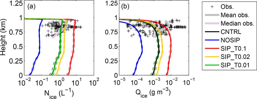
1304                             G. Sotiropoulou et al.: The impact of secondary ice production on Arctic stratocumulus

(e.g., Phillips et al., 2017b), but these are computationally    Cloud–rain drop processes are treated following Seifert and
expensive, and thus weather forecast and climate models typ-     Beheng (2001), while liquid–ice interactions are parameter-
ically incorporate bulk microphysical representations. It is     ized following Wang and Chang (1993). A simple parame-
likely that a property-based ice microphysics scheme, like       terization for CCN activation is applied (Khvorostyanov and
the predicted particle properties (P3) scheme (Morrison and      Curry, 2006), where the number of cloud droplets formed is
Milbrandt, 2015; Milbrandt and Morrison, 2016) in WRF,           a function of supersaturation and background aerosol con-
can support a more realistic representation of the BR pro-       centration (NCCN ). Ice nucleation is also parameterized fol-
cess. This scheme tracks the ice mixing ratio, number, mass      lowing DeMott et al. (2010). To account for INP loss due to
and rime fraction rather than the number and mass in snow,       activation, the newly nucleated crystals at each time step are
graupel and ice crystal categories, as in bulk schemes, whose    estimated by taking the INP number (NINP ) minus the num-
thresholds can be non-physical. However, in the current ver-     ber of existing ICNCs; this is a standard method applied in
sion of WRF, P3 considers only two ice categories, while         microphysics schemes that do not treat INPs as a prognos-
at least three are needed for the BR description (Yano and       tic variable (e.g., Morrison et al., 2005). CCN and INP con-
Phillips, 2011).                                                 centrations are passively advected within the model domain
   For the above reasons, we combine, for our investigations,    and not depleted through droplet activation or ice nucleation
a LPM specifically developed for the study of SIP (Sullivan      processes. A detailed radiation solver (Fu and Liou, 1992) is
et al., 2017, 2018a) and the MISU–MIT Cloud and Aerosol          coupled to MIMICA to account for cloud radiative properties
(MIMICA) LES (Savre et al., 2015), designed for the study        when calculating the radiative fluxes.
of Arctic clouds. The LPM allows for an adequate descrip-           All simulations are performed on a 96×96×128 grid, with
tion of the formation, growth and evolution of cloud droplets    constant horizontal spacing dx = dy = 62.5 m. The simu-
and ice particles as they interact with each other, including    lated domain is 6 km×6 km horizontally and 1.77 km verti-
SIP. The LES provides a three-dimensional description of the     cally. At the surface and in the cloud layer, the vertical grid
cloud system at a high spatial and temporal resolution, which    spacing is 7.5 m, while between the surface and the cloud
is of a similar scale to the observations. The LPM – driven by   base, it changes sinusoidally, reaching a maximum spacing
the LES conditions – is used to quantify the enhancement in      of 25 m. The integration time step is variable, calculated
ICNCs due to SIP compared to primary ice formation. The          continuously to satisfy the Courant–Friedrichs–Lewy crite-
ice crystal concentration in the LES (which includes only        rion for the leapfrog method. Lateral boundary conditions
a description of primary ice) is then enhanced by the LPM        are periodic, while a sponge layer in the top 500 m of the
result. This coupling between the LES and LPM occurs at          domain damps vertically propagating gravity waves sponta-
every time step throughout the simulation and constitutes a      neously generated during the simulations. To accelerate the
convenient way to combine the benefits of a computationally      development of turbulent motions, the initial ice–liquid po-
inexpensive bin model with the high-resolution LES. A de-        tential temperature profiles are randomly perturbed in the
tailed description of the modeling components and the over-      first 20 vertical grid levels with an amplitude not exceeding
all modeling methods and set-up are described below.             0.0003 K.

3.1    Large-eddy simulation (LES)                               3.2   Lagrangian parcel model (LPM)

The MIMICA LES (Savre et al., 2015) solves a set of non-         The ice enhancement from SIP is estimated with a LPM
hydrostatic prognostic equations for the conservation of mo-     with six hydrometeor classes for small, medium and large ice
mentum, ice–liquid potential temperature and total water         and liquid hydrometeors (Sullivan et al., 2017, 2018a). Al-
mixing ratio with an anelastic approximation. A fourth-order     though the bin microphysics is relatively coarsely resolved,
central finite-differences formulation determines momentum       it has served as a convenient framework for the study of ice
advection, and a second-order flux-limited version of the        multiplication and especially of the BR process (Yano and
Lax–Wendroff scheme (Durran, 2010) is employed for scalar        Phillips, 2011; Sullivan et al., 2018a).
advection. Equations are integrated forward in time using a         The six hydrometeor number tendencies are solved with
second-order leapfrog method and a modified Asselin filter       an explicit Runge–Kutta pair for delay differential equations
(Williams, 2010). Sub-grid-scale turbulence is parameterized     (Bogacki and Shampine, 1989) and coupled to moist ther-
using the Smagorinsky–Lilly eddy-diffusivity closure (Lilly,     modynamic equations for pressure, temperature, supersat-
1992), and surface fluxes are calculated according to Monin–     uration, liquid water and ice mixing ratios, and hydrome-
Obukhov similarity theory.                                       teor sizes; moist thermodynamic equations are solved with
   Cloud microphysics are described using a two-moment ap-       a second-order Rosenbrock solver (Rosenbrock, 1963). CCN
proach for cloud droplets, rain and ice particles. Mass mix-     activation is represented in the same way as in the LES, while
ing ratios and number concentrations are treated prognosti-      INP concentration is also constrained based on the LES re-
cally for these three hydrometeor classes, whereas their size    sults (see Text S1 and Fig. S1 in Supplement). Each resolved
distributions are defined by generalized Gamma functions.        hydrometeor type is represented by a characteristic size that

Atmos. Chem. Phys., 20, 1301–1316, 2020                                           www.atmos-chem-phys.net/20/1301/2020/
G. Sotiropoulou et al.: The impact of secondary ice production on Arctic stratocumulus                                              1305

is allowed to dynamically vary over time as a function of        ited precipitation (generally
1306 G. Sotiropoulou et al.: The impact of secondary ice production on Arctic stratocumulus
However, their experimental set-up was very simplified using
centimeter-sized hail balls, while one of the two colliding hy-
drometeors remained fixed. In our LPM simulations the ice
particles in the medium bin grow from 100 µm into millime-
ter sizes (not shown); thus using the above formula would
certainly lead to overestimation of the number of fragments
produced. For this reason, scaling FBR by a factor of 10–100
for size differences is essential (see Sect. 3.4 for a discus-
sion).
A more physically based parameterization for BR has been
recently developed by Phillips et al. (2017a), which estimates
FBR as a function of collisional kinetic energy and depends
on the colliding particles’ size and rimed fraction. This re-
sults in varying treatment of FBR for different ice crystal
types and ice habits. Since this parameterization requires sev-
eral parameters that are not available in our LPM (e.g., ice
particle type, habit and rimed fraction), for its implementa-
tion a number of assumptions have to be made. First of all,
since primary ice particles grow through vapor deposition
and move to the second bin, we assume that this bin rep-
resents snow. Given the relatively warm temperature range
(Pruppacher and Klett, 1997) and after inspection of particle
images, planar ice is likely the most representative ice habit
of the ACCACIA case. A rimed fraction of 0.4 is also as-
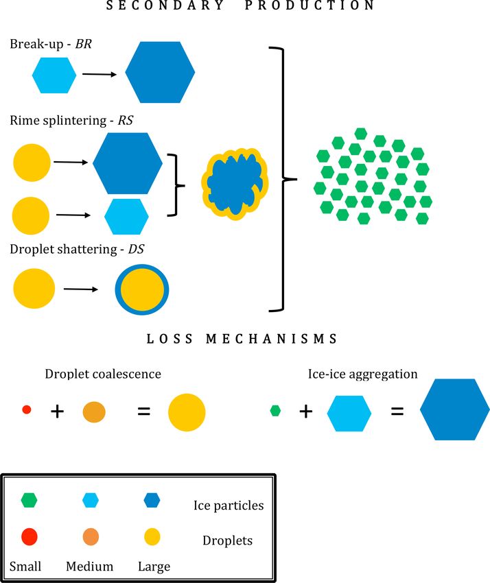
sumed, as lower values do not yield any SIP; FBR becomes Figure 3. Schematic representation of the simplified six-bin micro-
less than unity, and ICNCs are highly underestimated. Fi- physics (adapted from Sullivan et al., 2017).
nally, the third LPM bin is assumed to consist of sufficiently
rimed particles; thus the collision type adapted in our simu-
lation is that of snow–graupel:
Drop shattering is described as function of a freezing prob-
CKo γ
FBR = αA 1 − exp − , (5) ability (pfr ), parameterized following Paukert et al. (2017),
αA and a shattering probability (psh ) based on droplet levitation
m m 2 experiments conducted by Leisner et al. (2014):
where Ko = mgg+mGG uG − ug ,
!
1.33 × 10 −4 FDS = 2.5 × 10⁻¹¹ (2rR )4 pfr psh . (7)
A = 1.58 × 10⁷ 1 + 1009 2 1 + ,
D 1.5
γ = 0.5 − 0.259, Freezing is allowed only when raindrop size exceeds 100 µm,
and psh is a normal distribution centered at −15 ◦ C, with a
C = 7.08 × 10⁶ ψ, standard deviation of 10 ◦ C.
ψ = 3.5 × 10⁻³ , The number balance in each class is the generation func-
tion at the current time as a source and the generation func-
a = π Ds2 , (6)
tion at a time delay as the sink, along with aggregation and
and where Ds is the equivalent spherical diameter of the coalescence processes. Note that aggregation occurs between
smaller ice particle which undergoes fracturing, α is its sur- small and medium ice particles and generates new particles in
face area and 9 is the rimed fraction. C is the asperity– the largest bin. Similarly, coalescence removes droplets from
fragility coefficient, and ψ is a correction term for the ef- the small and medium bins and generates new ones in the
fects of sublimation in field observations by Vardiman et large raindrop category. A schematic of all these processes is
al. (1978). The above description concerns collisions of shown in Fig. 3.
either planar crystals or snow, with 9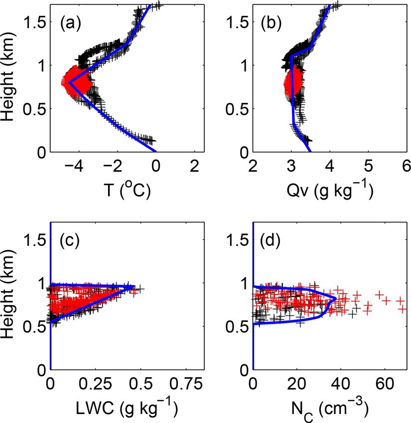
G. Sotiropoulou et al.: The impact of secondary ice production on Arctic stratocumulus                                       1307

3.3   Initial and boundary conditions                               we further perform sensitivity simulations by increasing this
                                                                    factor (see Sects. 3.4 and 4.4).
                                                                       Initial specific humidity and pressure in the LPM are set
The atmospheric profiles used to initialize the LES are             to the values measured at the cloud base (3.1 g kg−1 and
based on in situ observations collected between 10:00 and           980 hPa, respectively). The LPM is then run over a wide
11:00 UTC on 23 July (Fig. 2), along the flight track shown         temperature and vertical velocity range to encompass the in-
in Fig. 1. The fact that the aircraft did not sample vertically     cloud variability encountered during the LES simulation (see
through the atmosphere but flew across a relatively large do-       Sect. 3.4). The maximum duration for LPM simulations is
main (9 km × 180 km) and over variable surface conditions           set to 60 min, but the simulation ends also when the parcel
(Fig. 1) creates some challenges for the design of the control      reaches the lowest cloud temperature observed near the cloud
simulation: measurements below the cloud layer and above            top, −6.5 ◦ C. This condition ensures that parcels do not reach
the temperature inversion (Fig. 2a) are collected over the          colder temperatures in the LPM than those encountered in the
ocean, whereas the cloud layer is mostly sampled over the           cloud simulated by the LES.
marginal-ice zones (MIZs) and the ice pack. However, the               The ice enhancement factors, defined as Nice /NINP , where
uncertainty arising from utilizing all these measurements to        Nice is the sum of ice number concentrations in all three bins,
construct the initial vertical profiles (Fig. 2) is not necessar-   are derived from the LPM calculations at the end of the sim-
ily larger than utilizing reanalysis data at a similarly coarse     ulation time. These factors are saved in look-up tables and
resolution.                                                         then used by the LES: the concentration of the nucleated ice
   Since our focus is on the cloud layer, we simulate ice-          particles in each LES column is multiplied at each model
covered surface conditions in the LES. The co-existent tem-         time step by an enhancement factor, which is a function of
perature and specific humidity inversions, associated with the      the cloud base temperature (Tcbh ) and the mean cloud updraft
cloud top height, as observed in Fig. 2, are typical charac-        velocity (W ).
teristics of the summertime Arctic PBL over sea ice (Sedlar
et al., 2012; Tjernström et al., 2012). Note that cloud char-       3.4   Sensitivity experiments
acteristics can vary depending on the surface type, i.e., if
it is open water, MIZ or thicker ice, as NC and ICNC are            The role of SIP during the ACCACIA case is investigated
about 40 %–45 % lower over open water than over ice dur-            with the LES, in which the SIP effect is parameterized
ing the examined case (not shown), suggesting that optically        through look-up tables that encompass the LPM results (see
thicker clouds persisted over the latter. For this reason we        Sect. 3.3). The LPM is run over a certain range of temper-
only use cloud measurements collected at latitudes higher           ature and vertical velocities, representative of the ACCA-
than 81.7◦ N (Fig. 1) and within a 9 km×33 km ice-covered           CIA conditions. These ranges are determined by the 3-D
area to evaluate the simulated cloud properties.                    fields produced by the LES. Hourly outputs of the 3-D LES
   The wind forcing is set by setting the geostrophic wind,         fields indicate that in-cloud updraft velocities vary between
constant with height, equal to the observed vertical mean           near zero and ∼ 1.4 m s−1 (Fig. S4a), while the mean W is
value of 5.8 m s−1 . The surface pressure is set to 1010 hPa,       ∼ 0.25 m s−1 and only 0.2 % of simulated W values exceed
linearly extrapolated from low-level pressure measurements.         0.5 m s−1 . The simulated cloud temperatures span from −6.5
The surface temperature is set to 0 ◦ C and surface moisture        to −1.5 ◦ C (Fig. S4a); the coldest temperatures are found just
to the saturation value, which reflects summer ice conditions.      below the cloud top, while the cloud base temperature varies
The surface albedo is set to 0.65, representative of the sea-       between −4 and −2 ◦ C. These results are indicative of very
ice melting season (Persson et al., 2002). In MIMICA, subsi-        weak convection. To cover all LES simulated conditions, the
dence is treated as a linear function of height: wLS = −DLS z,      LPM is run for Tcbh between −5 and −1 ◦ C and vertical ve-
where DLS is the large-scale divergence. DLS here is defined        locity, W , between 0.25 and 1.25 m s−1 , with a step value
through trial and error: to avoid rapid vertical cloud displace-    of 0.5 ◦ C and 0.25 m s−1 , respectively, to derive the ice en-
ments, we prescribe DLS = 3 × 10⁻⁶ s−1 .                            hancement factors.
   A NCCN concentration of 50 cm−3 is prescribed, based                The CNTRL simulation corresponds to the LES experi-
on measurements of cloud droplet concentrations over the            ment that accounts for all SIP processes, with BR being pa-
ice pack (Fig. 2d), while the sensitivity to this choice is         rameterized after Phillips et al. (2017a), as this is the only
further tested (see Sects. 3.4 and 4.3). Implementing the           physically based description available for this process. A
temperature-dependent DM parameterization in the LES,               simulation with no active SIP mechanism is also carried out,
with mean observed aerosol concentrations (0.6 cm−3 ) as in-        referred to as NOSIP in the text. A comparison of these sim-
put, results in the development of a purely liquid cloud layer      ulations is found in Sect. 4.1.
in the LES (see Sect. 4.4). Given that the uncertainty in the          To further examine the sensitivity of the CNTRL results
DM parameterization is about 1 order of magnitude (De-              to BR formulation, three additional sensitivity tests are pre-
Mott et al., 2010), we therefore assume a baseline simula-          sented in the same section. In these simulations RS and DS
tion where INP estimates are multiplied by a factor of 5, and       are parameterized as in CNTRL, but BR is now based on

www.atmos-chem-phys.net/20/1301/2020/                                                Atmos. Chem. Phys., 20, 1301–1316, 2020
1308 G. Sotiropoulou et al.: The impact of secondary ice production on Arctic stratocumulus
tive SIP mechanism. These LES simulations are referred to
as (a) CCN10 and CCN100 and (b) CCN10_NOSIP and
CCN100_NOSIP, respectively.
Finally, in Sect. 4.4 the sensitivity to primary ice nu-
cleation is examined. The standard DM parameterization
predicts concentrations < ∼ 0.03 L−1 for temperaturesG. Sotiropoulou et al.: The impact of secondary ice production on Arctic stratocumulus 1309
Table 1. Description of the LES experiments performed in this study.
LES experiment SIP process active NCCN INP
concentration concentration
(cm−3 ) (L−1 )
CNTRL RS, BR (Phillips parameterization) 50 DM × 5
NOSIP None 50 DM × 5
SIP_T0.1 RS, BR (Takahashi scaled with a factor of 10) 50 DM × 5
SIP_T0.02 RS, BR (Takahashi scaled with a factor of 50) 50 DM × 5
SIP_T0.01 RS, BR (Takahashi scaled with a factor of 100) 50 DM × 5
BR BR (Phillips) 50 DM × 5
BR_T0.1 BR (Takahashi scaled with a factor of 10) 10 DM × 5
BR_T0.02 BR (Takahashi scaled with a factor of 50) 50 DM × 5
BR_T0.01 BR (Takahashi scaled with a factor of 100) 50 DM × 5
RS RS 50 DM × 5
CCN10 RS, BR (Phillips) 10 DM × 5
CCN10_NOSIP None 10 DM × 5
CCN100 RS, BR (Phillips) 100 DM × 5
CCN100_NOSIP None 100 DM × 5
DM RS, BR (Phillips) 50 DM
DM_NOSIP None 50 DM
DM10 RS, BR (Phillips) 50 DM × 10
DM10_NOSIP None 50 DM × 10
DM100 RS, BR (Phillips) 50 DM × 100
DM100_NOSIP None 50 DM × 100
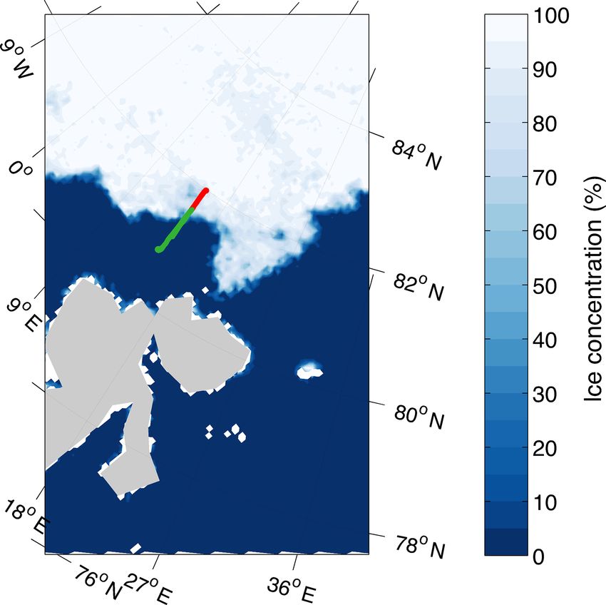
An interesting finding is that all simulations that account
for SIP produce ICNCs within the observed range, while
NOSIP clearly underestimates observations. These results
indicate that SIP can indeed explain the observed concen-
trations despite the uncertainties in BR parameterization.
The SIP_T0.02 simulation, which is in good agreement with
mean observations, represents fragmentation of 500 µm par-
ticles, while SIP_T0.01 is more representative of 100 µm
sizes. Phillips parameterization accounts for different sizes;
Figure 5. Vertical profiles of (a) ice crystal number concentration
however it is constrained by a specific collision type and
(Nice ) and (b) ice mass mixing ratio (Qice ) for CNTRL (black),
NOSIP (blue), SIP_T0.1 (red), SIP_T0.02 (yellow) and SIP_T0.01 specific particle properties (habit, rimed fraction, etc.). Nev-
(green) from the LES. Solid lines represent the mean profiles, av- ertheless, in reality more than one collision type can hap-
eraged between 4 and 8 h of simulation time, while dashed lines pen simultaneously, while the habit and rimed fraction of the
show the standard deviation. Black crosses represent the measure- particles that undergo fracturing can vary. Moreover, in our
ment range derived from the 2-D-S probe, while grey (pink) lines LPM each bin category is represented by a single diameter,
represent the observed mean (median) profiles. while observations indicate a broad particle size spectra, up
to 1.27 mm (Fig. S2b). Thus in reality micrometer-sized and
millimeter-sized particles can undergo break-up simultane-
however the modeled ICNCs can explain some of the largest ously, which might explain the wide range of observed IC-
values observed. SIP_T0.02 produces mean Nice and Qice NCs in Fig. 5a.
profiles in very good agreement with the mean observations,
while SIP_T0.01 performs similarly to CNTRL. The differ- 4.2 The role of the underlying SIP mechanisms
ences and similarities between these LES experiments are
also reflected in the LPM results (Text S2; Fig. S5): for the To quantify the contribution of each SIP mechanism, sim-
dominant thermodynamic conditions (W < ∼ 0.5 m s−1 and ulations that account for a single SIP mechanism are com-
−4 ◦ C1310 G. Sotiropoulou et al.: The impact of secondary ice production on Arctic stratocumulus
ditions it acts as a weaker source of secondary ice, which in
combination with RS can still significantly modulate the mi-
crophysical state of the cloud.
Following the formula of Yano and Phillips (2011), we
estimate the BR multiplication efficiency Ĉ = 4Co ã τg τG ,
where Co is the nucleation rate applied in the LPM and
ã = αFBR ; α is the sweep-out rate (adapted from Yano and
Phillips, 2011). Phillips et al. (2017a) and Takahashi et
al. (1995) parameterization, scaled with a factor 50–100, pre-
Figure 6. Same as in Fig. 5 but for the LES simulations with only dicts < ∼ 5 fragments per collision in the temperature range
one SIP mechanism active: BR (black), BR_T0.1 (red), BR_T0.02
of interest (Fig. 4); thus using the upper limit FBR = 5 in our
(yellow), BR_T0.01 (green) and RS (blue).
calculations yields Ĉ = 10.58, which is similar to the value
Ĉ = 10, predicted in Phillips et al. (2017b). Thus the theory
predicts an increase in the cloud ice concentration by a fac-
eterization predicts similar enhancement factors to Phillips tor of ∼ 10 over a timescale of about an hour; we assume
et al. (2017a) when implemented in the LPM (see Fig. S6). that this is likely the maximum efficiency of BR process in
BR_T0.02 has a more pronounced multiplication effect than Arctic stratocumulus, since 60 min is an upper cloud mixing
RS; however it still underestimates the mean and median ob- timescale for such clouds.
served profiles. BR_T0.1 is the only simulation that results
in similar mean cloud properties to the observed. 4.3 Sensitivity to CCN concentration
The weak multiplication effect in RS, BR and BR_T0.01 is
also clearly manifested in the LPM results (Text S2; Fig. S6),
In this section, we examine the sensitivity of our results to
which in weak updraft conditions produce enhancement fac-
the prescribed CCN concentration. The LES is run for two
tors < ∼ 5, while BR_T0.02 produces up to a 10-fold en-
additional NCCN conditions: 10 and 100 cm−3 (Fig. 7). The
hancement. The multiplication factor in BR_T0.1 can vary
look-up tables used to parameterize SIP in these simulations
between 10 and 100 times for ACCACIA conditions, result-
are shown in Fig. S7.
ing in improved LES results (Fig. 6) compared to the previ-
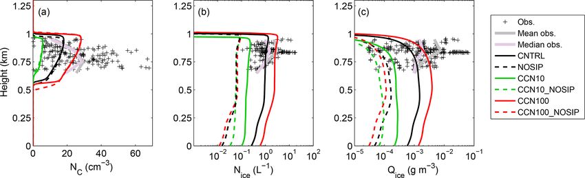
Distinct differences are observed in cloud droplet concen-
ous set-ups. However, in this simulation the results of Taka-
trations in Fig. 7a, which are significantly reduced with de-
hashi et al. (1995) are scaled assuming millimeter-sized par-
creasing NCCN along with a slight decrease in cloud thick-
ticles, which is rather an upper limit for the ice particle sizes
ness. There is no clear impact on cloud droplet number con-
measured during the campaign (Fig. S2b).
centrations when SIP is excluded. ICNCs in Fig. 7b are sim-
Figures 5–6 indicate a strong ice generation feedback be-
ilar for all simulations that do not account for SIP, while no
tween RS and BR, which results in substantially enhanced
substantial differences are observed in Qice profiles (Fig. 7c).
multiplication compared to the effect that each mechanism
In contrast, for the CNTRL, CCN10 and CCN100 simula-
can have when acting alone. The new fragments ejected dur-
tions, all produce clearly different results, suggesting that in-
ing rime splintering contribute to more ice–ice collisions
creasing CCN concentrations enhance SIP activity. This is
and thus further feed the BR multiplication process, which
mainly due to the increasing efficiency of RS, as more drops
eventually becomes more efficient than RS (not shown).
are formed to initiate this process (see Text S2; Fig. S7). All
Since BR is parameterized assuming millimeter-sized parti-
simulations accounting for SIP are in better agreement with
cles in BR_T0.1, which is the upper bound in observations
observations than those with no active SIP mechanism, sug-
(Fig. S2b), we suggest that the observed ICNCs are most
gesting that including a SIP parameterization can improve
likely caused by a combination of both mechanisms (Fig. 5a).
model performance for a variety of CCN conditions.
While RS has been extensively implemented in mesoscale
and climate models, this is not the case with BR; how-
ever, our results indicate that this is also an important SIP 4.4 Sensitivity to INP concentration
mechanism. Our findings are in contrast to the results of
Fu et al. (2019), who found that BR efficiency is limited Here we examine the sensitivity of our results to the INP
in mesoscale simulations of autumnal Arctic clouds. How- concentration by conducting six additional LES simulations:
ever, apart from focusing on different thermodynamic condi- DM, DM10 and DM100 and DM_NOSIP, DM10_NOSIP
tions, another difference is that they performed offline calcu- and DM100_NOSIP (see Table 1 for details). The vertical NC
lations of the BR effect using the parameterization of Vardi- profiles exhibit no substantial difference between all simula-
man (1978). Another interesting fact is that while other stud- tions except DM100, where the cloud appears geometrically
ies (Yano and Phillips, 2011, 2016) have shown that BR can thinner (Fig. 8a). This is due to the substantial ice concentra-
be highly effective at very cold temperatures (∼ −15 ◦ C), re- tion produced in this simulation, which results in glaciation
sulting even in explosive multiplication, in the examined con- of the lower portion of the cloud (Fig. 8b). Ice properties,
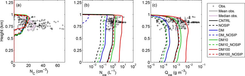
Atmos. Chem. Phys., 20, 1301–1316, 2020 www.atmos-chem-phys.net/20/1301/2020/G. Sotiropoulou et al.: The impact of secondary ice production on Arctic stratocumulus 1311 Figure 7. Vertical profiles of (a) cloud droplet concentrations (cm−3 ), (b) ice crystal concentrations (L−1 ) and (c) ice mass mixing ratio (g m−3 ) for the LES sensitivity simulations with varying NCCN . Black, green and red solid (dashed) lines represent CNTRL (NOSIP), CCN10 (CCN10_NOSIP) and CCN100 (CCN100_NOSIP) runs, respectively. The results are averaged between 4 and 8 h of simulation time. Black crosses represent the observations, while the solid grey lines show the median observed profile. however, exhibit distinct differences among all INP sensitiv- Qice range, suggesting that a SIP parameterization does not ity tests (Fig. 8b, c). degrade model performance even when unrealistically high The standard DeMott parameterization (DM) results in ice INP conditions are prescribed. properties in agreement with the lowest observed values. If no SIP is accounted for (DM_NOSIP), almost no ice is pro- duced (Fig. 8b, c). DM10 is in good agreement with the 5 Discussion and conclusions median observations (Fig. 8b, c); however, if SIP is deacti- vated (DM10_NOSIP), the results agree only with the lowest Semi-idealized simulations of Arctic stratocumulus clouds range of measurements. For extremely high INP conditions, observed during the ACCACIA campaign are performed to primary nucleation alone (DM100_NOSIP) can produce the investigate the impact of SIP using a LES and a LPM: the mean observed ICNCs, activating SIP results in mean con- LES provides a realistic representation of the atmospheric centrations of about 4–5 L−1 , while the simulated mean Qice thermodynamics, while the LPM provides a more simplified profile is close to the observed mean. framework to parameterize SIP. The effect of three SIP mech- The comparison of Nice profiles between DM and anisms, rime splintering (RS), collisional break-up (BR) and DM_NOSIP simulations suggests that the enhancement due drop shattering (DS), is investigated. Furthermore, the sensi- to SIP is about a factor of 50–100, while for CNTRL and tivity to the choice of the BR description is also examined, NOSIP (DM × 5) it is a factor of 15–20 (Fig. 8b). For DM10 using ice fragmentation rates from Phillips et al. (2017a) and and DM10_NOSIP the enhancement is also about 1 order Takahashi et al. (1995); the first parameterization is more ad- of magnitude, while it is somewhat smaller when compar- vanced, accounting for changes in collisional kinetic energy ing DM100 and DM100_NOSIP (Fig. 8b). Thus in the LES of the colliding particles, while the latter is a more simpli- simulations, SIP enhancement decreases with increasing pri- fied temperature-dependent relationship. Our simulations in- mary ice nucleation. In contrast to the LES, the LPM results dicate that SIP processes are essential to reproduce the ob- suggest that increasing INP concentrations result in more ef- served ICNCs, which are well above the concentrations gen- fective SIP (Fig. S8); this result is somewhat expected, since erated by primary ice nucleation. Good agreement with ob- larger concentrations of primary ice crystals would result in served values of cloud ice properties is obtained when either more frequent ice–ice collisions (Text S2; Fig. S8). However, of the BR descriptions is employed, as long as the formula the LES simulations indicate that processes that act as sinks derived from Takahashi et al. (1995) is properly scaled for for ice concentrations, such as precipitation, become more size and a high rimed fraction is prescribed in Phillips pa- effective with increasing Nice and Qice . rameterization. All in all, these sensitivity simulations indicate that con- When the contribution of each mechanism is examined sidering SIP processes in the LES results in an overall better separately, DS is found to be ineffective, which is in good representation of the cloud ice properties for a variety of INP agreement with previous studies of Arctic clouds (Fu et al., conditions. Note that the uncertainty in the DM parameteri- 2019). Moreover, both RS and BR are weak when being the zation is about a factor of 10 (DeMott et al., 2010), and simu- only active SIP mechanism. The limited influence of RS is lations that predict primary ice within this uncertainty range due to the lack of relatively large raindrops to initiate this are in better agreement with the observations when SIP is ac- process. RS has also been found insufficient to explain ob- tive. It is interesting to note that even the unrealistic case of served ICNCs in Antarctic stratocumulus clouds in a simi- DM100 still produces results within the observed Nice and lar temperature range (Young et al., 2019). To reproduce the www.atmos-chem-phys.net/20/1301/2020/ Atmos. Chem. Phys., 20, 1301–1316, 2020
1312                                G. Sotiropoulou et al.: The impact of secondary ice production on Arctic stratocumulus

Figure 8. Same as Fig. 7 but for the LES sensitivity simulations with varying INP concentration. Black, blue, green and red solid (dashed)
lines represent CNTRL (NOSIP), DM (DM_NOSIP), DM10 (DM_NOSIP) and DM100 (DM100_NOSIP) experiments, respectively.

observations, Young et al. (2019) had to remove the liquid             assumed a constant number of fragments generated when
thresholds from the RS parameterization that allow RS acti-            snow collides with graupel. However, this approach may re-
vation only when sufficiently large droplets are formed. Fur-          sult in significantly underestimated SIP, as other types of col-
thermore, they had to multiply the RS efficiency by a factor           lisions that include large ice crystals may occur (Phillips et
of 10. The limited efficiency of BR is due to a lack of enough         al., 2017a). Sullivan et al. (2018b) did consider collisions be-
primary ice crystals to initiate ice–ice collisions. Our results       tween ice crystals and the other two hydrometeor types in a
indicate that the combination of both RS and BR is a pos-              similar bulk scheme in COSMO-ART, using the original (un-
sible explanation for the observed ICNCs; the newly gener-             scaled) formula of Takahashi et al. (1995). However, their ap-
ated fragments by RS further fuel the BR process, resulting            proach may instead result in an overestimated BR efficiency,
in substantial ice enhancement through the latter, compared            as not all crystal sizes are suitable to fuel this process, includ-
to when only one mechanism is active. Interestingly, when              ing the very small fragments generated by BR. Nevertheless,
only RS is accounted for, the multiplication effect has to be          one of the most important outcomes of this study is that the
increased by about a factor of 10–20 to obtain a good agree-           simple framework of the LPM, when it is driven (“tuned”)
ment with the observed ICNCs, i.e., the same factor as that            by the LES thermodynamic fields, provides ice number en-
used in Young et al. (2019).                                           hancement factors that bridge the model results with obser-
   Our results here indicate that at relatively warm sub-              vations. This suggests that the LPM, when appropriately con-
zero temperatures and in low updraft conditions, BR is a               strained by observations (or LES-type simulations), provides
potentially important ice production mechanism, particu-               a promising approach towards parameterizing SIP in large-
larly in combination in RS. BR efficiency in Arctic condi-             scale models.
tions has been also documented in observational studies of                Our results indicate that BR is likely a critical mechanism
mixed-phase clouds in the past (Rangno and Hobbs, 2001;                in Arctic stratocumulus clouds, where large drops are sparse
Schwarzenboeck et al., 2009). Schwarzenboeck et al. (2009)             and RS efficiency is limited. Thus a correct representation
analyzed measurements collected with a Cloud Particle Im-              of this process in models will likely alleviate some of the
ager during the ASTAR (Arctic Study of Aerosols, Clouds                model deficiencies in representing cloud ice properties and
and Radiation) campaign and found evidence of stellar-                 hence the shortwave radiation budget (Young et al., 2019).
crystal fragmentation in 55 % of the samples; 18 % of these            However, existing parameterizations are based on old labora-
cases were attributed to natural fragmentation, while for the          tory datasets and simplified experimental set-ups (Vardiman,
rest, 82 %, the possibility of artificial fragmentation (e.g.,         1978; Takahashi et al., 1995). As there have been significant
shattering on the probe) could not be excluded. Moreover,              advances in the development of laboratory instruments suit-
they only included stellar crystals with sizes > ∼ 300 µm in           able for BR studies in the past decades, we highlight the need
their analysis, suggesting that their estimate for natural crys-       for new laboratory experiments with more realistic set-ups
tal fragmentation frequency is likely underestimated.                  that focus on the BR mechanism. We believe that constrain-
   Despite the potential significance of BR, very few attempts         ing BR accurately in models could have a significant impact
have been made to include this process in large-scale models.          on the representation of Arctic climate in large-scale models
Hoarau et al. (2018) recently incorporated BR into Meso-               and projections for the future.
NH, which includes a two-moment microphysics scheme
with three ice hydrometeor types: ice crystal, graupel and
snow particles, whose sizes are determined by gamma dis-
tributions (as in most bulk schemes). To represent BR, they

Atmos. Chem. Phys., 20, 1301–1316, 2020                                                  www.atmos-chem-phys.net/20/1301/2020/
G. Sotiropoulou et al.: The impact of secondary ice production on Arctic stratocumulus                                                    1313

Code and data availability. The original LPM code can be found at           spheric Data Centre, date of citation, http://catalogue.ceda.ac.uk/
https://github.com/scs2229/SIM (last access: December 2019; Sul-            uuid/c59f184de7a408212ee926a9ee6bf66e (last access: January
livan, 2019). The LES code is available upon request.                       2020), 2014.
   ACCACIA observations are available at https://data.bas.ac.uk/         British Antarctic Survey: Data from the ACCACIA – Aerosol-
metadata.php?id=GB/NERC/BAS/PDC/00821 (last access: Jan-                    Cloud Coupling And Climate Interactions in the Arctic project,
uary 2020; British Antarctic Survey, 2015) and https://catalogue.           available at: https://data.bas.ac.uk/metadata.php?id=GB/NERC/
ceda.ac.uk/uuid/c59f184de7a408212ee926a9ee6bf66e (last access:              BAS/PDC/00821 (last access: January 2020), 2015.
January 2020; British Antarctic Survey, 2014).                           Brown, P. and Francis, P.: Improved measurements of the ice wa-
                                                                            ter content in cirrus using a total-water probe, J. Atmos. Ocean.
                                                                            Tech., 12, 410–414, 1995.
Supplement. The supplement related to this article is available on-      Choularton, T. W., Griggs, D. J., Humood, B. Y.,
line at: https://doi.org/10.5194/acp-20-1301-2020-supplement.               and Latham, J.: Laboratory studies of riming, and its relation to
                                                                            ice splinter production, Q. J. Roy. Meteor. Soc., 106, 367–374,
                                                                            https://doi.org/10.1002/qj.49710644809, 1980.
Author contributions. GS and AN conceived and led this study.            Crawford, I., Bower, K. N., Choularton, T. W., Dearden, C., Crosier,
AMLE and JS provided the LES code, while SS wrote the origi-                J., Westbrook, C., Capes, G., Coe, H., Connolly, P. J., Dorsey,
nal LPM code. GL and TLC provided the ACCACIA observations.                 J. R., Gallagher, M. W., Williams, P., Trembath, J., Cui, Z.,
GS performed the LPM and LES simulations, analyzed the results,             and Blyth, A.: Ice formation and development in aged, win-
and, together with AN wrote the main paper. AMLE, SS and JS                 tertime cumulus over the UK: observations and modelling, At-
were also involved in the scientific interpretation and discussion and      mos. Chem. Phys., 12, 4963–4985, https://doi.org/10.5194/acp-
commented on the paper.                                                     12-4963-2012, 2012.
                                                                         Crosier, J., Choularton, T. W., Westbrook, C. D., Blyth, A. M.,
                                                                            Bower, K. N., Connolly, P. J., Dearden, C., Gallagher, M. W.,
                                                                            Cui, Z., and Nicol, J. C.: Microphysical properties of cold
Competing interests. The authors declare that they have no conflict
                                                                            frontal rainbands, Q. J. Roy. Meteorol. Soc., 140, 1257–1268,
of interest.
                                                                            https://doi.org/10.1002/qj.2206, 2013.
                                                                         DeMott, P. J., Prenni, A. J., Liu, X., Kreidenweis, S. M., Petters, M.
                                                                            D., Twohy, C. H., Richardson, M. S., Eidhammer, T., and Rogers,
Acknowledgements. We acknowledge support from the Laboratory                D. C.: Predicting global atmospheric ice nuclei distributions and
of Atmospheric Processes and their Impacts at the École Polytech-           their impacts on climate, P. Natl. Acad. Sci., 107, 11217–11222,
nique Fédérale de Lausanne, Switzerland (http://lapi.epfl.ch, last ac-      https://doi.org/10.1073/pnas.0910818107, 2010.
cess: January 2020) and the project PyroTRACH (ERC-2016-COG)             Durran, D. R.: Numerical Methods for Fluid Dynamics, Texts Appl.
funded by H2020-EU.1.1. – Excellent Science – European Research             Math., 2nd ed., Springer, Berlin-Heidelberg, Germany, 2010.
Council. We are also grateful to the ACCACIA scientific crew for         Ferrier, B. S.: A Double-Moment Multiple-Phase Four-
the observational datasets used in this study and to the two anony-         Class Bulk Ice Scheme. Part I: Description, J. At-
mous reviewers for constructive comments.                                   mos. Sci., 51, 249–280, https://doi.org/10.1175/1520-
                                                                            0469(1994)0512.0.CO;2, 1994.
                                                                         Field, P., Lawson, P., Brown, G., Lloyd, C., Westbrook, D.,
Financial support. This research has been supported by the H2020-           Moisseev, A., Miltenberger, A., Nenes, A., Blyth, A., Choular-
EU.1.1. (grant no. 726165).                                                 ton, T., Connolly, P., Bühl, J., Crosier, J., Cui, Z., Dearden, C.,
                                                                            DeMott, P., Flossmann, A., Heymsfield, A., Huang, Y., Kalesse,
                                                                            H., Kanji, Z., Korolev, A., Kirchgaessner, A., Lasher-Trapp, S.,
Review statement. This paper was edited by Johannes Quaas and               Leisner, T., McFarquhar, G., Phillips, V., Stith, J., and Sullivan,
reviewed by two anonymous referees.                                         S.: Chapter 7: Secondary ice production – current state of the
                                                                            science and recommendations for the future, Meteor. Monogr.,
                                                                            58, 7.1–7.20, https://doi.org/10.1175/AMSMONOGRAPHS-D-
                                                                            16-0014.1, 2017.
References                                                               Fridlind, A. M., Ackerman, A. S., McFarquhar, G., Zhang, G., Poel-
                                                                            lot, M. R., DeMott, P. J., Prenni, A. J., and Heymsfield, A. J.: Ice
Barton, N. P., Klein, S. A., and Boyle, J. S.: On the Contribu-             properties of single-layer stratocumulus during the Mixed-Phase
  tion of Longwave Radiation to Global Climate Model Biases in              Arctic Cloud Experiment: 2. Model results., J. Geophys. Res.,
  Arctic Lower Tropospheric Stability, J. Clim., 27, 7250–7269,             112, D24202, https://doi.org/10.1029/2007JD008646, 2007.
  https://doi.org/10.1175/JCLI-D-14-00126.1, 2014.                       Déry, S. J. and Yau, M. K.: A Climatology of Adverse Winter-Type
Bogacki, P. and Shampine, L. F.: A 3(2) pair of Runge-Kutta formu-          Weather Events, J. Geophys. Res., 104, 16657–16672,1999.
  las, Appl. Math. Lett., 2, 321–325, https://doi.org/10.1016/0893-      Fu, Q. and Liou, K. N: On the Correlated k-Distribution Method
  9659(89)90079-7, 1989.                                                    for Radiative Transfer in Nonhomogeneous Atmospheres, J. At-
British Antarctic Survey: Facility for Airborne Atmospheric Mea-            mos., 49, 2139–2156, https://doi.org/10.1007/s00382-016-3040-
  surements, Met Office, Liu, D., McFiggans, G. B., Allan, J. D.:           8, 1992.
  Aerosol-Cloud Coupling And Climate Interactions in the Arc-
  tic (ACCACIA) Measurement Campaign, NCAS British Atmo-

www.atmos-chem-phys.net/20/1301/2020/                                                       Atmos. Chem. Phys., 20, 1301–1316, 2020
1314 G. Sotiropoulou et al.: The impact of secondary ice production on Arctic stratocumulus Fu, S., Deng, X., Shupe, M. D., and Huiwen, X.: A mod- Korolev, A. V., Emergy, E., and Creelman, K.: Modification and elling study of the continuous ice formation in an autum- Tests of Particle Probe Tips to Mitigate Effects of Ice Shattering, nal Arctic mixed-phase cloud case, Atmos. Res., 228, 77–85, J. Atmos. Ocean. Tech., 30, 690–708, 2013. https://doi.org/10.1016/j.atmosres.2019.05.021, 2019. Lauber, A., Kiselev, A., Pander, T., Handmann, P., and Leisner, T.: Gayet, J. F., Treffeisen, R., Helbig, A., Bareiss, J., Matsuki, A., Her- Secondary ice formation during freezing of levitated droplets, J. ber, A., and Schwarzenboeck, A.: On the onset of the ice phase Atmos. Sci., 75, 2815–2826, https://doi.org/10.1175/JAS-D-18- in boundary layer Arctic clouds, J. Geophys. Res., 114, D19201, 0052.1, 2018. https://doi.org/10.1029/2008JD011348, 2009. Lawson, R. P., Woods, S., and Morrison, H.: The microphysics of Gettelman, A., Liu, X., Ghan, S. J., Morrison, H., Park, S., Con- ice and precipitation development in tropical cumulus clouds, J. ley, A. J., Klein, S. A., Boyle, J., Mitchell, D. L., and Li, Atmos. Sci., 72, 2429–2445, https://doi.org/10.1175/JAS-D-14- J.-L. F.: Global simulations of ice nucleation and ice su- 0274.1, 2015. persaturation with an improved cloud scheme in the Com- Lawson, P., Gurganus, C., Woods, S., and Bruintjes, R.: Aircraft ob- munity Atmosphere Model, J. Geophys. Res., 115, D18216, servations of cumulus microphysics ranging from the tropics to https://doi.org/10.1029/2009JD013797, 2010. midlatitudes: implications for a “new” secondary ice process, J. Gossart, A., Souverijns, N., Gorodetskaya, I. V., Lhermitte, S., Atmos. Sci., 74, 2899–2920, https://doi.org/10.1175/JAS-D-17- Lenaerts, J. T. M., Schween, J. H., Mangold, A., Laffineur, 0033.1, 2017. Q., and van Lipzig, N. P. M.: Blowing snow detection from Leisner, T., Pander, T., Handmann, P., and Kiselev, A.: Secondary ground-based ceilometers: application to East Antarctica, The ice processes upon heterogeneous freezing of cloud droplets, Cryosphere, 11, 2755–2772, https://doi.org/10.5194/tc-11-2755- 14th Conf. on Cloud Physics and Atmospheric Radiation, Amer. 2017, 2017. Meteor. Soc, Boston, MA, 2014. Hallett, J. and Mossop, S. C.: Production of secondary ice Li, G., Wang, Y., and Zhang, R.:Implementation of a twomo- particles during the riming process, Nature, 249, 26–28, ment bulk microphysics scheme to the WRF model to investi- https://doi.org/10.1038/249026a0, 1974. gate aerosolcloud interaction, J. Geophys. Res., 113, D15211, Hoarau, T., Pinty, J.-P., and Barthe, C.: A representation of the col- https://doi.org/10.1029/2007JD009361, 2008. lisional ice break-up process in the two-moment microphysics Lilly, D. K.: A proposed modification to the Germano LIMA v1.0 scheme of Meso-NH, Geosci. Model Dev., 11, 4269– subgrid-scale closure method, Phys. Fluids, 4, 633–635, 4289, https://doi.org/10.5194/gmd-11-4269-2018, 2018. https://doi.org/10.1063/1.858280, 1992. Heymsfield, A. J. and Mossop, S. C.: Temperature depen- Lloyd, G., Choularton, T. W., Bower, K. N., Gallagher, M. W., denceof secondary ice crystal production during soft hail- Connolly, P. J., Flynn, M., Farrington, R., Crosier, J., Sch- growth by riming, Q. J. Roy. Meteor. Soc., 110, 765–770, lenczek, O., Fugal, J., and Henneberger, J.: The origins of https://doi.org/10.1002/qj.49711046512, 1984. ice crystals measured in mixed-phase clouds at the high- Jensen, A. A. and Harrington, J. Y.: Modeling ice crystal aspect alpine site Jungfraujoch, Atmos. Chem. Phys., 15, 12953–12969, ratio evolution during riming: A single-particle growth model, J. https://doi.org/10.5194/acp-15-12953-2015, 2015. Atmos. Sci., 72, 2569–2590, https://doi.org/10.1175/JAS-D-14- Mignani, C., Creamean, J. M., Zimmermann, L., Alewell, C., and 0297.1, 2015. Conen, F.: New type of evidence for secondary ice formation at Jung, C. H., Yoon, Y. J., Kang, H. J., Gim, Y., Lee, around −15 ◦ C in mixed-phase clouds, Atmos. Chem. Phys., 19, B. Y., Ström, J., Krejci, R., and Tunved, P.: The sea- 877–886, https://doi.org/10.5194/acp-19-877-2019, 2019. sonal characteristics of cloud condensation nuclei (CCN) Milbrandt, J. A. and Morrison, H.: Parameterization of Cloud Mi- in the arctic lower troposphere, Tellus B, 70, 1–13, crophysics Based on the Prediction of Bulk Ice Particle Prop- https://doi.org/10.1080/16000889.2018.1513291, 2018. erties. Part III: Introduction of Multiple Free Categories, J. Karlsson, J. and Svensson, G.: Consequences of poor representation Atmos. Sci., 73, 975–995, https://doi.org/10.1175/JAS-D-15- of Arctic sea-ice albedo and cloud-radiation interactions in the 0204.1, 2016. CMIP5 model ensemble, Geophys. Res. Lett., 40, 4374–4379, Morrison, H. and Milbrandt, J. A.: Parameterization of Cloud https://doi.org/10.1002/grl.50768, 2013. Microphysics Based on the Prediction of Bulk Ice Particle Khvorostyanov, V. I. and Curry, J. A.: Fall velocities of hy- Properties. Part I: Scheme Description and Idealized Tests, J. drometeors in the atmosphere: Refinements to a continu- Atmos. Sci., 72, 287–311, https://doi.org/10.1175/JAS-D-14- ous analytical power law, J. Atmos. Sci., 62, 4343–4357, 0065.1, 2015. https://doi.org/10.1175/JAS3622.1, 2006. Morrison, H., Curry, J. A., and Khvorostyanov, V. I.: A New Korolev, A., McFarquhar, G., Field, P. R., Franklin, C., Lawson, Double-Moment Microphysics Parameterization for Application P., Wang, Z., Williams, E., Abel, S. J., Axisa, D., Borrmann, S., in Cloud and Climate Models. Part I: Description, Atmos. Sci., Crosier, J., Fugal, J., Krämer, M., Lohmann, U., Schlenczek, 62, 3683–3704, 2005. O., Schnaiter, M., and Wendisch, M.: Mixed-Phase Clouds: Morrison, H., de Boer, G., Feingold, G., Harrington, J., Progress and Challenges, Meteorol. Monogr., 58, 5.1–5.50, Shupe, M. D., and Sulia, K.: Resilience of persistent https://doi.org/10.1175/AMSMONOGRAPHS-D-17-0001.1, Arctic mixed-phase clouds, Nature Geosci., 5, 11–17, 2017. https://doi.org/10.1038/ngeo1332, 2012. Korolev, A. V., Emery, E. F., Strapp, J. W., Cober, S. G., Isaac, G. A., Paukert, M., Hoose, C., and Simmel, M.: Redistribution of ice nu- Wasey, M., and Marcotte, D.: Small ice particles in tropospheric clei between cloud and rain droplets: parameterization and ap- clouds: fact or artifact?, B. Am. Meteorol. Soc., 92, 967–973, plication to deep convective clouds, J. Adv. Model. Earth Sy., 9, https://doi.org/10.1175/2010BAMS3141.1, 2011. 514–535, https://doi.org/10.1002/2016MS000841, 2017. Atmos. Chem. Phys., 20, 1301–1316, 2020 www.atmos-chem-phys.net/20/1301/2020/
You can also read