The GPU version of LASG/IAP Climate System Ocean Model version 3 (LICOM3) under the heterogeneous-compute interface for portability (HIP) ...
←
→
Page content transcription
If your browser does not render page correctly, please read the page content below
Geosci. Model Dev., 14, 2781–2799, 2021
https://doi.org/10.5194/gmd-14-2781-2021
© Author(s) 2021. This work is distributed under
the Creative Commons Attribution 4.0 License.

The GPU version of LASG/IAP Climate System Ocean Model
version 3 (LICOM3) under the heterogeneous-compute interface
for portability (HIP) framework and its large-scale application
Pengfei Wang1,3 , Jinrong Jiang2,4 , Pengfei Lin1,4 , Mengrong Ding1 , Junlin Wei2 , Feng Zhang2 , Lian Zhao2 , Yiwen Li1 ,
Zipeng Yu1 , Weipeng Zheng1,4 , Yongqiang Yu1,4 , Xuebin Chi2,4 , and Hailong Liu1,4
1 StateKey Laboratory of Numerical Modeling for Atmospheric Sciences and Geophysical Fluid Dynamics (LASG),
Institute of Atmospheric Physics (IAP), Chinese Academy of Sciences (CAS), Beijing 100029, China
2 Computer Network Information Center, Chinese Academy of Sciences, Beijing 100190, China
3 Center for Monsoon System Research (CMSR), Institute of Atmospheric Physics, Chinese Academy of Sciences,

Beijing 100190, China
4 University of Chinese Academy of Sciences, Beijing 100049, China

Correspondence: Jinrong Jiang (jjr@sccas.cn), Pengfei Lin (linpf@mail.iap.ac.cn), and Hailong Liu (lhl@lasg.iap.ac.cn)

Received: 25 September 2020 – Discussion started: 10 December 2020
Revised: 8 April 2021 – Accepted: 12 April 2021 – Published: 18 May 2021

Abstract. A high-resolution (1/20◦ ) global ocean gen-            results suggests that the 1/20◦ LICOM3-HIP can reproduce
eral circulation model with graphics processing unit (GPU)        the observations and produce many smaller-scale activities,
code implementations is developed based on the LASG/IAP           such as submesoscale eddies and frontal-scale structures.
Climate System Ocean Model version 3 (LICOM3) un-
der a heterogeneous-compute interface for portability (HIP)
framework. The dynamic core and physics package of LI-
COM3 are both ported to the GPU, and three-dimensional            1   Introduction
parallelization (also partitioned in the vertical direction) is
applied. The HIP version of LICOM3 (LICOM3-HIP) is 42             Numerical models are a powerful tool for weather fore-
times faster than the same number of CPU cores when 384           casts and climate prediction and projection. Creating high-
AMD GPUs and CPU cores are used. LICOM3-HIP has ex-               resolution atmospheric, oceanic, and climatic models re-
cellent scalability; it can still obtain a speedup of more than   mains a significant scientific and engineering challenge be-
4 on 9216 GPUs compared to 384 GPUs. In this phase, we            cause of the enormous computing, communication, and in-
successfully performed a test of 1/20◦ LICOM3-HIP us-             put and/or output (IO) involved. Kilometer-scale weather and
ing 6550 nodes and 26 200 GPUs, and on a large scale, the         climate simulation have recently started to emerge (Schär
model’s speed was increased to approximately 2.72 simu-           et al., 2020). Due to the considerable increase in computa-
lated years per day (SYPD). By putting almost all the com-        tional cost, such models will only work with extreme-scale
putation processes inside GPUs, the time cost of data transfer    high-performance computers and new technologies.
between CPUs and GPUs was reduced, resulting in high per-            Global ocean general circulation models (OGCMs) are a
formance. Simultaneously, a 14-year spin-up integration fol-      fundamental tool for oceanography research, ocean forecast-
lowing phase 2 of the Ocean Model Intercomparison Project         ing, and climate change research (Chassignet et al., 2019).
(OMIP-2) protocol of surface forcing was performed, and           Such model performance is determined mainly by model
preliminary results were evaluated. We found that the model       resolution and subgrid parameterization and surface forcing.
results had little difference from the CPU version. Further       The horizontal resolution of global OGCMs has increased
comparison with observations and lower-resolution LICOM3          to approximately 5–10 km, and these models are also called
                                                                  eddy-resolving models. Increasing the resolution will sig-

Published by Copernicus Publications on behalf of the European Geosciences Union.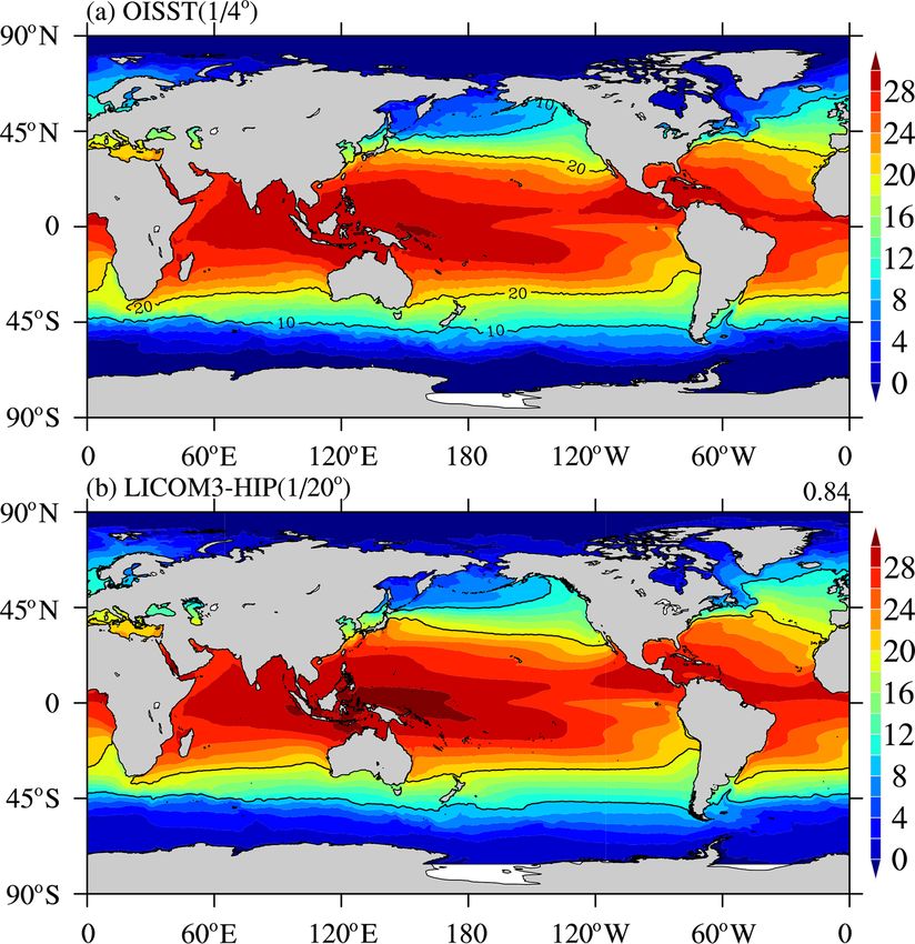
2782             P. Wang et al.: The GPU version of LICOM3 under the HIP framework and its large-scale application

nificantly improve the simulation of western boundary cur-       solution to address this problem. It provides a higher-level
rents, mesoscale eddies, fronts and jets, and currents in nar-   framework to contain these two types of lower-level de-
row passages (Hewitt et al., 2017). Meanwhile, the ability of    velopment environments, i.e., CUDA and HCC, simultane-
an ocean model to simulate the energy cascade (Wang et al.,      ously. The HIP code’s grammar is similar to that of the
2019), the air–sea interaction (Hewitt et al., 2017), and the    CUDA code, and with a simple conversion tool, the code
ocean heat uptake (Griffies et al., 2015) will be improved       can be compiled and run at CUDA and AMD architects.
with increasing resolution. All these factors will effectively   HCC/OpenACC (Open ACCelerators) is more convenient for
improve ocean model performance in the simulation and pre-       AMD GPU developers than the HIP, which is popular from
diction of ocean circulation. Additionally, the latest numeri-   the coding viewpoint. Another reason is that CUDA GPUs
cal and observational results show that much smaller eddies      currently have more market share. It is believed that an in-
(submesoscale eddies with a spatial scale of approximately       creasing number of codes will be ported to the HIP in the
5–10 km) are crucial to vertical heat transport in the upper-    future. However, almost no ocean models use the HIP frame-
ocean mixed layer and significant to biological processes (Su    work to date.
et al., 2018). Resolving the smaller-scale processes raises         This study aims to develop a high-performance OGCM
a new challenge for the horizontal resolution of OGCMs,          based on the LASG/IAP Climate System Ocean Model ver-
which also demands much more computing resources.                sion 3 (LICOM3), which can be run on an AMD GPU archi-
   Heterogeneous computing has become a development              tecture using the HIP framework. Here, we will focus on the
trend of high-performance computers. In the latest TOP500        model’s best or fastest computing performance and its prac-
supercomputer list released in November 2020 (https://www.       tical usage for research and operation purposes. Section 2
top500.org/lists/top500/2020/11/, last access: 17 May 2021),     is the introduction of the LICOM3 model. Section 3 con-
central processing unit (CPU) and graphics processing unit       tains the main optimization of LICOM3 under HIP. Section 4
(GPU) heterogeneous machines account for 6 of the top            covers the performance analysis and model verification. Sec-
10. After the NVIDIA Corporation provided supercomputing         tion 5 is a discussion, and the conclusion is presented in
techniques on GPUs, an increasing number of ocean mod-           Sect. 6.
els applied these high-performance acceleration methods to
conduct weather or climate simulations. Xu et al. (2015)
developed POM.gpu (GPU version of the Princeton Ocean            2     The LICOM3 model and experiments
Model), a full GPU solution based on mpiPOM (MPI version
of the Princeton Ocean Model) on a cluster, and achieved a       2.1    The LICOM3 model
6.8 times energy reduction. Yashiro et al. (2016) deployed the
NICAM (Nonhydrostatic ICosahedral Atmospheric Model)             In this study, the targeting model is LICOM3, which was
on the TSUBAME supercomputer, and the model sustained a          developed in the late 1980s (Zhang and Liang, 1989). Cur-
double-precision performance of 60 teraflops on 2560 GPUs.       rently, LICOM3 is the ocean model for two air–sea cou-
Yuan et al. (2020) developed a GPU version of a wave             pled models of CMIP6 (the Coupled Model Intercomparison
model with 2 V100 cards and obtained a speedup of 10–            Project phase 6), the Flexible Global Ocean-Atmosphere-
12 times when compared to the 36 cores of the CPU. Yang          Land System model version 3 with a finite-volume atmo-
et al. (2016) implemented a fully implicit β-plane dynamic       spheric model (FGOALS-f3; He et al., 2020), and the Flex-
model with 488 m grid spacing on the TaihuLight system and       ible Global Ocean-Atmosphere-Land System model version
achieved 7.95 petaflops. Fuhrer et al. (2018) reported a 2 km    3 with a grid-point atmospheric model (Chinese Academy of
regional atmospheric general circulation model (AGCM) test       Science, CAS, FGOALS-g3; L. Li et al., 2020). LICOM ver-
using 4888 GPU cards and obtained a simulation perfor-           sion 2 (LICOM2.0, Liu et al., 2012) is also the ocean model
mance for 0.043 simulated years per wall clock day (SYPD).       of the CAS Earth System Model (CAS-ESM, H. Zhang et al.,
S. Zhang et al. (2020) successfully ported a high-resolution     2020). A future paper to fully describe the new features and
(25 km atmosphere and 10 km ocean) Community Earth Sys-          baseline performances of LICOM3 is in preparation.
tem Model in the TaihuLight supercomputer and obtained 1–           In recent years, the LICOM model was substantially im-
3.4 SYPD.                                                        proved based on LICOM2.0 (Liu et al., 2012). There are
   Additionally, the AMD company also provides GPU so-           three main aspects. First, the coupling interface of LICOM
lutions. In general, AMD GPUs use heterogeneous compute          has been upgraded. Now, the NCAR flux coupler version 7
compiler (HCC) tools to compile codes, and they cannot use       is employed (Lin et al., 2016), in which memory use has
the Compute Unified Device Architecture (CUDA) develop-          been dramatically reduced (Craig et al., 2012). This makes
ment environments, which provide support for the NVIDIA          the coupler suitable for application to high-resolution mod-
GPU only. Therefore, due to the wide use and numerous            eling.
CUDA learning resources, AMD developers must study two              Second, both orthogonal curvilinear coordinates (Murray,
kinds of GPU programming skills. AMD’s heterogeneous-            1996; Madec and Imbard, 1996) and tripolar grids have been
compute interface for portability (HIP) is an open-source        introduced in LICOM. Now, the two poles are at 60.8◦ N,

Geosci. Model Dev., 14, 2781–2799, 2021                                         https://doi.org/10.5194/gmd-14-2781-2021
P. Wang et al.: The GPU version of LICOM3 under the HIP framework and its large-scale application                             2783

65◦ E and 60.8◦ N, 115◦ W for the 1◦ model, at 65◦ N, 65◦ E          tails of these models are listed in Table 1. The number of hor-
and 65◦ N, 115◦ W for the 0.1◦ model, and at 60.4◦ N, 65◦ E          izontal grid points for the three configurations are 360 × 218,
and 60.4◦ N, 115◦ W for the 1/20◦ model of LICOM. Af-                3600 × 2302, and 7200 × 3920. The vertical levels for the
ter that, the zonal filter at high latitudes, particularly in the    low-resolution models are 30, while they are 55 for the other
Northern Hemisphere, was eliminated, which significantly             two high-resolution models. From 1◦ to 1/20◦ , the compu-
improved the scalability and efficiency of the parallel algo-        tational effort increased by approximately 8000 (203 ) times
rithm of the LICOM3 model. In addition, the dynamic core             (considering 20 times to decrease the time step), and the ver-
of the model has also been updated accordingly (Yu et al.,           tical resolution increased from 30 to 55, in total, by approx-
2018), including the application of a new advection scheme           imately 15 000 times. The original CPU version of 1/20◦
for the tracer formulation (Xiao, 2006) and the addition of a        with MPI (Message Passing Interface) parallel on Tianhe-1A
vertical viscosity for the momentum formulation (Yu et al.,          only reached 0.31 SYPD using 9216 CPU cores. This speed
2018).                                                               will slow down the 10-year spin-up simulation of LICOM3
   Third, the physical package has been updated, including           to more than 1 month, which is not practical for climate
introducing an isopycnal and thickness diffusivity scheme            research. Therefore, such simulations require extreme-scale
(Ferreira et al., 2005) and vertical mixing due to internal          high-performance computers by applying the GPU version.
tides breaking at the bottom (St. Laurent et al., 2002). The            In addition to the different grid points, three main aspects
coefficient of both isopycnal and thickness diffusivity is           are different among the three experiments, particularly be-
set to 300 m2 s−1 as the depth is either within the mixed            tween version 1◦ and the other two versions. First, the hor-
layer or the water depth is shallower than 60 m. The up-             izontal viscosity schemes are different: using Laplacian for
per and lower boundary values of the coefficient are 2000            1◦ and biharmonic for 1/10◦ and 1/20◦ . The viscosity co-
and 300 m2 s−1 , respectively. Additionally, the chlorophyll-        efficient is 1 order of magnitude smaller for the 1/20◦ ver-
dependent solar shortwave radiation penetration scheme of            sion than for the 1/10◦ version, namely, −1.0 × 10⁹ m4 s−1
Ohlmann (2003), the isopycnal mixing scheme (Redi, 1982;             for 1/10◦ vs. −1.0 × 10⁸ m4 s−1 for 1/20◦ . Second, although
Gent and McWilliams, 1990), and the vertical viscosity and           the force-including dataset (the Japanese 55-year reanalysis
diffusivity schemes (Canuto et al., 2001, 2002) are employed         dataset for driving ocean–sea-ice models, JRA55-do; Tsu-
in LICOM3.                                                           jino et al., 2018) and the bulk formula for the three exper-
   Both the low-resolution (1◦ ; Lin et al., 2020) and high-         iments are all a standard of the OMIP-2, the periods and
resolution (1/10◦ ; Y. Li et al., 2020) stand-alone LICOM3           temporal resolutions of the forcing fields are different: 6 h
versions are also involved in the Ocean Model Intercom-              data from 1958 to 2018 for the 1◦ version and daily mean
parison Project (OMIP)-1 and OMIP-2; their outputs can be            data in 2016 for both the 1/10◦ and 1/20◦ versions. Third,
downloaded from websites. The two versions of LICOM3’s               version 1◦ is coupled with a sea ice model of CICE4 (Com-
performances compared with other CMIP6 ocean models are              munity Ice CodE version 4.0) via the NCAR flux coupler
shown in Tsujino et al. (2020) and Chassignet et al. (2020).         version 7, while the two higher-resolution models are stand-
The 1/10◦ version has also been applied to perform short-            alone, without a coupler or sea ice model. Additionally, the
term ocean forecasts (Liu et al., 2021).                             two higher-resolution experiments employ the new HIP ver-
   The essential task of the ocean model is to solve the ap-         sion of LICOM3 (i.e., LICOM3-HIP); the low-resolution ex-
proximated Navier–Stokes equations, along with the con-              periment does not employ this, including the CPU version
servation equations of the temperature and salinity. Seven           of LICOM3 and the version submitted to OMIP (Lin et al.,
kernels are within the time integral loop, named “readyt”,           2020). We also listed all the important information in Table 1,
“readyc”, “barotr”, “bclinc”, “tracer”, “icesnow”, and “con-         such as bathymetry data and the bulk formula, although these
vadj”, which are also the main subroutines porting from the          items are similar in the three configurations.
CPU to the GPU. The first two kernels computed the terms                The spin-up experiments for the two high-resolution ver-
in the barotropic and baroclinic equations of the model. The         sions are conducted for 14 years, forced by the daily JRA55-
next three (barotr, bclinc, and tracer) are used to solve the        do dataset in 2016. The atmospheric variables include the
barotropic, baroclinic, and temperature and/or salinity equa-        wind vectors at 10 m, air temperature at 10 m, relative hu-
tions. The last two subroutines deal with sea ice and deep           midity at 10 m, total precipitation, downward shortwave ra-
convection processes at high latitudes. All these subroutines        diation flux, downward longwave radiation flux, and river
have approximately 12 000 lines of source code, accounting           runoff. According to the kinetic energy evolution, the mod-
for approximately 25 % of the total code and 95 % of com-            els reach a quasi-equilibrium state after more than 10 years
putation.                                                            of spin-up. The daily mean data are output for storage and
                                                                     analysis.
2.2   Configurations of the models

To investigate the GPU version, we employed three configu-
rations in the present study. They are 1◦ , 0.1◦ , and 1/20◦ . De-

https://doi.org/10.5194/gmd-14-2781-2021                                               Geosci. Model Dev., 14, 2781–2799, 2021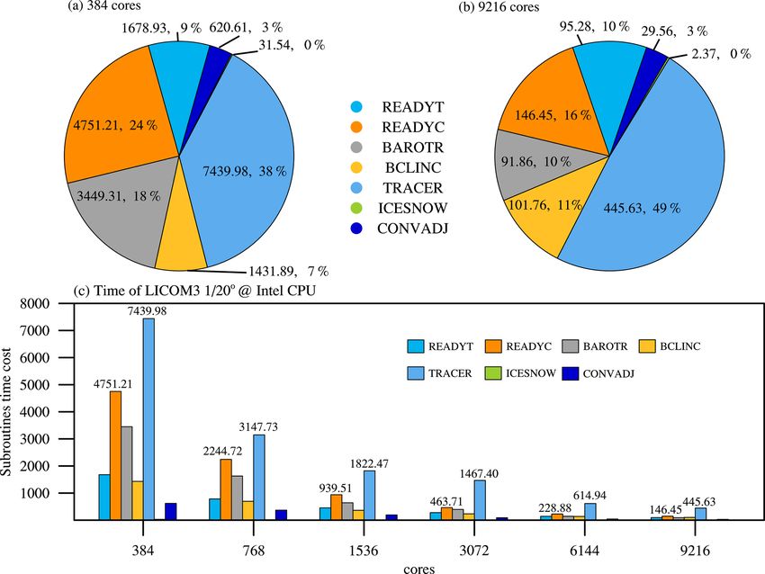
2784                  P. Wang et al.: The GPU version of LICOM3 under the HIP framework and its large-scale application

Table 1. Configurations of the LICOM3 model used in the present study.

 Experiment                                    LICOM3-CPU (1◦ )               LICOM3-HIP (1/10◦ )            LICOM3-HIP (1/20◦ )
 Horizontal grid spacing                       1◦ (110 km in longitude, ap-   1/10◦ (11 km in longitude,     1/20◦ (5.5 km in longitude,
                                               proximately 110 km at the      approximately 11 km at the     approximately 5.5 km at the
                                               Equator, and 70 km at mid-     Equator, and 7 km at mid-      Equator, and 3 km at mid-
                                               latitude)                      latitude)                      latitude)
 Grid point                                    360 × 218                      3600 × 2302                    7200 × 3920
 North Pole                                    60.8◦ N, 65◦ E and             65◦ N, 65◦ E and               60.4◦ N, 65◦ E and
                                               60.8◦ N, 115◦ W                65◦ N, 115◦ W                  60.4◦ N, 115◦ W
 Bathymetry data                               ETOPO2                         Same                           Same
 Vertical coordinates                          30η levels                     55η levels                     55η levels
 Horizontal viscosity                          Laplacian                      Biharmonic (Fox-Kemper         Biharmonic (Fox-Kemper
                                               A2 = 3000 m2 s−1               and Menemenlis, 2008)          and Menemenlis, 2008)
                                                                              A4 = −1.0 × 10⁹ m4 s−1         A4 = −1.0 × 10⁸ m4 s−1
 Vertical viscosity                            Background viscosity of        Background viscosity of        Background viscosity of
                                               2 × 10⁻⁶ m2 s−1       with     2 × 10⁻⁶ m2 s−1       with     2 × 10⁻⁶ m2 s−1       with
                                               the   upper    limit    of     the   upper    limit    of     the   upper    limit    of
                                               2 × 10⁻² m2 s−1                2 × 10⁻² m2 s−1                2 × 10⁻² m2 s−1
 Time steps                                    120/1440/1440                  6/120/120 s                    3/60/60 s
                                               for                            for                            for
                                               barotropic/baroclinic/tracer   barotropic/baroclinic/tracer   barotropic/baroclinic/tracer
 Bulk formula                                  Large and Yeager (2009)        Same                           Same
 Forcing data                                  JRA55_do, 1958–2018,           JRA55_do, 2016,                JRA55_do, 2016,
                                               6-hourly                       daily                          daily
 Integration period                            61 years/six cycles            14 years                       14 years
 Mixed layer scheme                            Canuto et al. (2001, 2002)     Same                           Same
 Isopycnal mixing                              Redi (1982);                   Laplacian                      Laplacian
                                               Gent and         McWilliams
                                               (1990)
 Bottom drag                                   Cb = 2.6 × 10⁻³                Cb = 2.6 × 10⁻³                Cb = 2.6 × 10⁻³
 Surface wind stress                           Relative wind stress           Same                           Same
 Sea surface temperature restoring timescale   20 m yr−1 ; 50 m 30 d−1 for    Same                           Same
                                               sea ice region
 Advection scheme                              Leapfrog for momentum;         Same                           Same
                                               two-step preserved shape
                                               advection scheme for tracer
 Time stepping scheme                          Split-explicit      leapfrog   Same                           Same
                                               with Asselin filter (0.2
                                               for barotropic; 0.43 for
                                               baroclinic; 0.43 for tracer)
 Sea ice                                       Sea ice model of CICE4         Not coupled                    Not coupled
 Ref.                                          Lin et al. (2020)              This paper                     This paper

Geosci. Model Dev., 14, 2781–2799, 2021                                                    https://doi.org/10.5194/gmd-14-2781-2021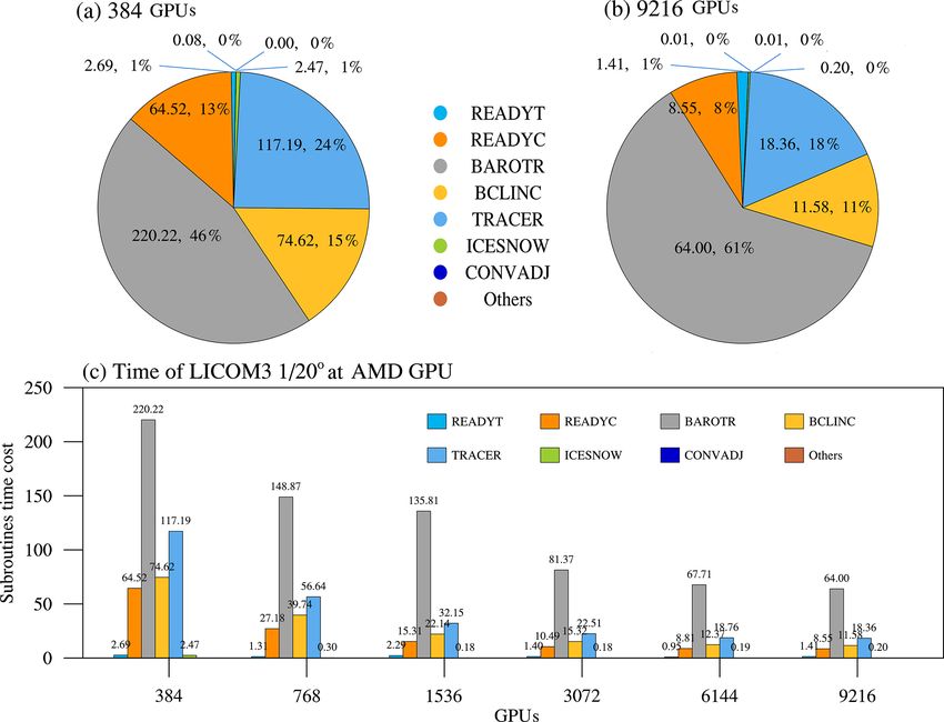
P. Wang et al.: The GPU version of LICOM3 under the HIP framework and its large-scale application                         2785

2.3    Hardware and software environments of the testing
       system

The two higher-resolution experiments were performed on
a heterogeneous Linux cluster supercomputer located at the
Computer Network Information Center (CNIC) of the CAS,
China. This supercomputer consists of 7200 nodes (six par-
titions or rings; each partition has 1200 nodes), with a
1.9 GHz X64 CPU of 32 cores on each node. Additionally,
each node is equipped with four gfx906 AMD GPU cards
with 16 GB memory. The GPU has 64 cores, for a to-
tal of 2560 threads on each card. The nodes are intercon-
nected through high-performance InfiniBand (IB) networks
(three-level fat-tree architecture using Mellanox 200 GB s−1      Figure 1. Schematic diagram of the comparison of coding on AMD
HDR (High Dynamic Range) InfiniBand, whose measured               and NVIDIA GPUs at three levels.
point-to-point communication performance is approximately
23 GB s−1 ). OpenMPI (Open Multi-Processing) version 4.02
was employed for compiling, and the AMD GPU driver and            ences in naming and libraries, there are other differences be-
libraries were rocm-2.9 (Radeon Open Computing platform           tween HIP and CUDA including the following: (1) the AMD
version 2.9), integrated with HIP version 2.8. The storage file   Graphics Core Next (GCN) hardware “warp” size is 64; (2)
system of the supercomputer is ParaStor300S with a “paras-        device and host pointers allocated by HIP API use flat ad-
tor” file system, whose measured write and read performance       dressing (unified virtual addressing is enabled by default);
is approximately 520 and 540 GB s−1 , respectively.               (3) dynamic parallelism is not currently supported; (4) some
                                                                  CUDA library functions do not have AMD equivalents; and
                                                                  (5) shared memory and registers per thread may differ be-
3     LICOM3 GPU code structure and optimization                  tween the AMD and NVIDIA hardware. Despite these differ-
                                                                  ences, most of the CUDA codes in applications can be easily
3.1    Introduction to HIP on an AMD hardware                     translated to the HIP and vice versa.
       platform                                                      Technical supports of CUDA and HIP also have some
                                                                  differences. For example, CUDA applications have some
AMD’s HIP is a C++ runtime API (application program-              CUDA-aware MPI to direct MPI communication between
ming interface) and kernel language. It allows developers to      different GPU memory spaces at different nodes, but HIP
create portable applications that can be run on AMD accel-        applications have no such functions to date. Data must be
erators and CUDA devices. The HIP provides an API for             transferred from GPU memory to CPU memory in order to
an application to leverage GPU acceleration for both AMD          exchange data with other nodes and then transfer data back
and CUDA devices. It is syntactically similar to CUDA, and        to the GPU memory.
most CUDA API calls can be converted by replacing the
character “cuda” with “hip” (or “Cuda” with “Hip”). The           3.2   Core computation process of LICOM3 and C
HIP supports a strong subset of CUDA runtime function-                  transitional version
ality, and its open-source software is currently available on
GitHub (https://rocmdocs.amd.com/en/latest/Programming_           We attempted to apply LICOM on a heterogeneous computer
Guides/HIP-GUIDE.html, last access: 17 May 2021).                 approximately 5 years ago, cooperating with the NVIDIA
   Some supercomputers install NVIDIA GPU cards, such             Corporation. LICOM2 was adapted to NVIDIA P80 by Ope-
as P100 and V100, and some install AMD GPU cards, such            nACC Technical (Jiang et al., 2019). This was a convenient
as AMD VERG20. Hence, our HIP version LICOM3 can                  implementation of LICOM2-gpu (GPU version of LICOM2)
adapt and gain very high performance at different super-          using four NVIDIA GPUs to achieve a 6.6 speedup com-
computer centers, such as Tianhe-2 and AMD clusters. Our          pared to four Intel CPUs, but its speedup was not as good
coding experience on an AMD GPU indicates that the HIP            when further increasing the GPU number.
is a good choice for high-performance model development.             During this research, we started from the CPU version
Meanwhile, the model version is easy to keep consistent           of LICOM3. The code structure of LICOM3 includes four
in these two commonly used platforms. In the following            steps. The first step is the model setup, which involves MPI
sections, the successful simulation of LICOM3-HIP is con-         partitioning and ocean data distribution. The second stage is
firmed to be adequate to employ HIP.                              model initialization, which includes reading the input data
   Figure 1 demonstrates the HIP implementations necessary        and initializing the variables. The third stage is integration
to support different types of GPUs. In addition to the differ-    loops or the core computation of the model. Three explicit

https://doi.org/10.5194/gmd-14-2781-2021                                            Geosci. Model Dev., 14, 2781–2799, 2021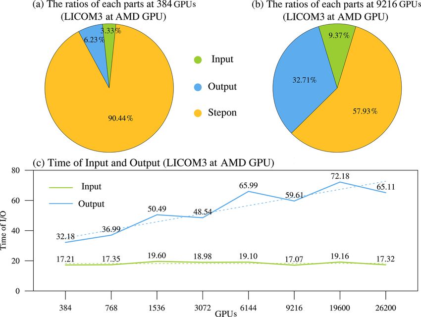
2786               P. Wang et al.: The GPU version of LICOM3 under the HIP framework and its large-scale application

Figure 2. LICOM3 computation flowchart with a GPU (HIP de-
vice). The red line indicates whole block data transfer between the     Figure 3. The wall clock time of a model day for the 10 km version
host and GPU, while the blue line indicates transferring only lateral   and a model month for the 100 km version. The blue and orange
data of a block.                                                        bars are for the Fortran and Fortran and C mixed versions. These
                                                                        tests were conducted on an Intel Xeon CPU platform (E5-2697A v4,
                                                                        2.60 GHz). We used 28 and 280 cores for the low and high resolu-
time loops, which are for tracer, baroclinic and barotropic             tions, respectively.
steps, are undertaken in 1 model day. The outputs and final
processes are included in the fourth step.
   Figure 2 shows the flowchart of LICOM3. The major pro-               the model (i.e., the same hardware and software conduct the
cesses within the model time integration include baroclinic,            same result). The C transitional version (not fully C code,
barotropic, and thermohaline equations, which are solved by             but the seven core subroutines) is bit-reproducible with the
the leapfrog or Euler forward scheme. There are seven indi-             F90 version of LICOM3 (the binary output data are the same
vidual subroutines: readyt, readyc, barotr, bclinc, tracer, ices-       under Linux with the “diff” command). We also tested the
now, and convadj. When the model finishes 1 d computation,              execution time. The Fortran and C hybrid version’s speed is
the diagnostics and output subroutine will write out the pre-           slightly faster (less than 10 %) than the original Fortran code.
dicted variables to files. The output files contain all the nec-        Figure 3 shows a speed benchmark by LICOM3 for 100 and
essary variables to restart the model and for analysis.                 10 km running on an Intel platform. The results are the wall
   To obtain high performance, it is more efficient to use the          clock time of running 1 model month for a low-resolution
native GPU development language. In the CUDA develop-                   test and 1 model day for a high-resolution test. The details of
ment forum, both CUDA-C and CUDA-Fortran are provided;                  the platform are found in the caption of Fig. 3. The results in-
however, Fortran’s support is not as efficient as that for C++.         dicate that we successfully ported these kernels from Fortran
We plan to push all the core process codes into GPUs; hence,            to C.
the seven significant subroutines’ Fortran codes must be con-              This C transitional version becomes the starting point of
verted to HIP/C++. Due to the complexity and many lines                 HIP/C++ codes and reduces the complexity of developing
in these subroutines (approximately 12 000 lines of Fortran             the HIP version of LICOM3.
code) and to ensure that the converted C/C++ codes are cor-
rect, we rewrote them to C before finally converting them to            3.3   Optimization and tuning methods in LICOM3-HIP
HIP codes.
   A bit-reproducible climate model produces the same nu-               The unit of computation in LICOM3-HIP is a horizontal grid
merical results for a given precision, regardless of the choice         point. For example, 1/20◦ corresponds to 7200 × 3920 grids.
of domain decomposition, the type of simulation (contin-                For the convenience of MPI parallelism, the grid points are
uous or restart), compilers, and the architectures executing            grouped as blocks; that is, if Procx × Procy MPI processes

Geosci. Model Dev., 14, 2781–2799, 2021                                                  https://doi.org/10.5194/gmd-14-2781-2021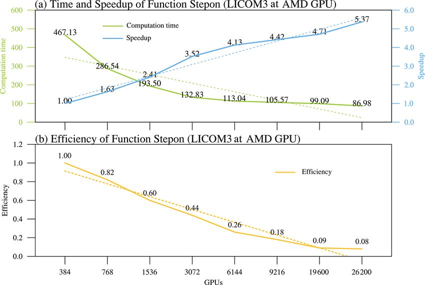
P. Wang et al.: The GPU version of LICOM3 under the HIP framework and its large-scale application 2787
Table 2. Block partition for the 1/20◦ setup. Table 3. The number calls of halos in LICOM3 subroutines for each
step.
GPUs Bx × By imt × j mt
Subroutine Calls Call percentage
384 600 × 124 604 × 128
768 600 × 62 604 × 66 barotr 180 96.7 %
1536 300 × 62 304 × 66 bclinc 2 1.1 %
3072 150 × 62 154 × 66 tracer 4 2.2 %
6144 100 × 62 104 × 66
9216 75 × 62 79 × 66
19 600 36 × 40 40 × 44
26 200 36 × 30 40 × 34 tions are needed to adapt to this change, such as increasing
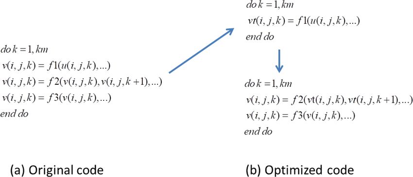
the global arrays to avoid data dependency. A demo for us-
ing a temporary array to parallelize the computation inside a
block is shown in Fig. 4. Figure 4a represents a loop of the
are used in the x and y directions, then each block has original code in the k direction. Since the variable v(i, j, k)
Bx × By grids, where Procx × Bx = 7200 and Procy × By = has a dependence on v(i, j, k +1), it will cause an error when
3920. Each GPU process performs two-dimensional (2-D) or the GPU threads are parallel in the k direction. We then sep-
three-dimensional (3-D) computations in these Bx ×By grids, arate the variable into two HIP kernel computations. In the
which is similar to the MPI process. Two-dimensional means upper part of Fig. 4b, a temporary array vt is used to hold the
that the grids are partitioned only in the horizontal directions, result of f 1(), and this can be GPU threads that are parallel
and 3-D includes also the depth or vertical direction. In prac- in the k direction. Then, at the bottom of Fig. 4b, we use vt
tice, four lateral columns are added to Bx and By (two on to perform the computations of f 2() and f 3(); this can still
each side, imt = Bx + 4, j mt = By + 4) for the halo. Table 2 be GPU threads that are parallel in the k direction. Finally,
lists the frequently used block definitions of LICOM3. this loop of codes is parallelized.
The original LICOM3 was written in F90. To adapt it to a Parallelization in a GPU is similar to a shared-memory
GPU, we applied Fortran–C hybrid programming. As shown program; memory write conflicts occur in the subroutine
in Fig. 2, the codes are kept using the F90 language be- tracer advection computation. We change the if–else tree in
fore entering device stepon and after stepon out. The core this subroutine; hence, the data conflicts between neighbor-
computation processes within the stepons are rewritten using ing grids are avoided, making the 3-D parallelism successful.
HIP/C. Data structures in the CPU space remain the same Moreover, in this subroutine, we use more operations to al-
as the original Fortran structures. The data commonly used ternate the data movement to reduce the cache usage. Since
by F90 and C are then defined by extra C, including files, the operation can be GPU thread parallelized and will not
and defined by “extern”-type pointers in C syntax to refer to increase the total computation time, reducing the memory
them. In the GPU space, newly allocated GPU global mem- cache improves this subroutine’s final performance.
ories hold the arrival correspondence with those in the CPU A notable problem when the resolution is increased to
space, and the HipMemcpy is called to copy them in and out. 1/20◦ is that the total size of Fortran common blocks will
Seven major subroutines (including their sub-recurrent be larger than 2 GB. This change will not cause abnormal-
calls) are converted from Fortran to HIP. The seven subrou- ities for C in the GPU space. However, if the GPU pro-
tine call sequences are maintained, but each subroutine is cess references the data, the system call in HipMemcpy will
deeply recoded in the HIP to obtain the best performance. cause compilation errors (perhaps due to the compiler limi-
The CPU space data are 2-D or 3-D arrays; in the GPU space, tation of the GPU compilation tool). We can change the orig-
they are changed to 1-D arrays to improve the data transfer inal Fortran arrays’ data structure from the “static” to the
speed between different GPU subroutines. “allocatable” type in this situation. Since a GPU is limited
LICOM3-HIP is a two-level parallelism, and each MPI to 16 GB GPU memory, the ocean block size in one block
process corresponds to an ocean block. The computation should not be too large. In practice, the 1/20◦ version starts
within one MPI process is then pushed into the GPU. The from 384 GPUs (and is regarded as the baseline for speedup
latency of the data copy between the GPU and CPU is one here); if the partition is smaller than that value, sometimes
of the bottlenecks for daily computation loops. All read-only insufficient GPU memory errors will occur.
GPU variables are allocated and copied at the initial stage to We found that the tracer is the most time-consuming sub-
reduce the data copy time. Some data copy is still needed in routine for the CPU version (Fig. 5). With the increase in
the stepping loop, e.g., an MPI call in barotr.cpp. CPU cores from 384 to 9216, the ratio of cost time for the
The computation block in MPI (corresponding to 1 GPU) tracer also increases from 38 % to 49 %. The subroutines
is a 3-D grid; in the HIP revision, 3-D parallelism is imple- readyt and readyc are computing-intensive. The subroutine
mented. This change adds more parallels inside one block tracer is both a computing-intensive and communication-
than the MPI solo parallelism (only 2-D). Some optimiza- intensive, and barotr is a communication-intensive subrou-
https://doi.org/10.5194/gmd-14-2781-2021 Geosci. Model Dev., 14, 2781–2799, 2021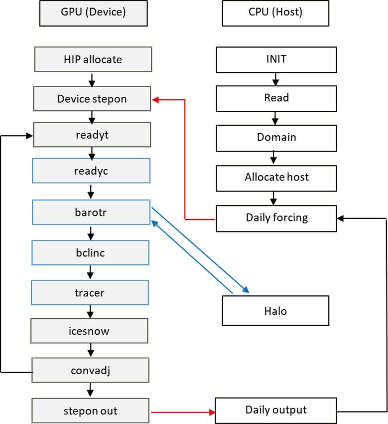
2788               P. Wang et al.: The GPU version of LICOM3 under the HIP framework and its large-scale application

Figure 4. The code using temporary arrays to avoid data dependency.

Figure 5. The seven core subroutines’ time cost percentages for (a) 384 and (b) 9216 CPU cores. (c) The subroutines’ time cost at different
scales of LICOM3 (1/20◦ ). These tests were conducted on an Intel Xeon CPU platform (E5-2697A v4, 2.60 GHz).

tine. The communication of barotr is 45 times more than                 figure shows that barotr is the most time-consuming subrou-
that of tracer (Table 3). Computing-intensive subroutines               tine, and the memory copy dominates, which takes approxi-
can achieve good GPU speed, but communication-intensive                 mately 40 % of the total time cost.
subroutines will achieve poor performance. The superlinear                 Data operations inside CPU (or GPU) memory are at least
speedups for tracer and readyc might be mainly caused by                1 order of magnitude faster than the data transfer between
memory use, in which the memory use of each thread for                  GPU and CPU through 16X PCI-e. Halo exchange at the
768 GPU cards is only half for 384 GPU cards.                           MPI level is similar to POP (Jiang et al., 2019). We did not
   We performed a set of experiments to measure the time                change these codes in the HIP version. The four blue rows
cost of both halo update and memory copy in the HIP ver-                and columns in Fig. 7 demonstrate the data that need to be
sion (Fig. 6). These two processes in the time integration are          exchanged with the neighbors. As shown in Fig. 7, in GPU
conducted in three subroutines: barotr, bclinc, and tracer. The         space, we pack the necessary lateral data for halo operation

Geosci. Model Dev., 14, 2781–2799, 2021                                                  https://doi.org/10.5194/gmd-14-2781-2021
P. Wang et al.: The GPU version of LICOM3 under the HIP framework and its large-scale application                                   2789

                                                                         cost for reading daily forcing data from the disk increased
                                                                         to 200 s in 1 model day after the model resolution increased
                                                                         from 1 to 1/20◦ . This time is comparable to the wall clock
                                                                         time for one model step when 1536 GPUs are applied; hence,
                                                                         we must optimize the model for total speedup. The cause
                                                                         of low performance is daily data reading and scattering to
                                                                         all nodes every model day; we then rewrite the data reading
                                                                         strategy and perform parallel scattering for 10 different forc-
                                                                         ing variables. Originally, 10 variables are read from 10 files,
                                                                         interpolated to a 1/20◦ grid, and then scattered to each pro-
                                                                         cessor or thread. All the processes are sequentially done at
                                                                         the master processor. In the revised code, we use 10 different
                                                                         processes to read, interpolate, and scatter in parallel. Finally,
                                                                         the time cost of input is reduced to approximately 20 s, which
                                                                         is 1/10 of the original time cost (shown below).
                                                                            As indicated, the time cost for one integration step (ex-
                                                                         cluding the daily mean and I/O) is approximately 200 s using
                                                                         1536 GPUs. One model day’s output needs approximately
                                                                         250 s; this is also beyond the GPU computation time for one
                                                                         step. We modify the subroutine to a parallel version, which
                                                                         decreases the data write time to 70 s on the test platform (this
                                                                         also depends on system I/O performance).

                                                                         4     Model performance

                                                                         4.1    Model performance in computing

Figure 6. The ratio of the time cost of halo update and memory           Performing kilometer-scale and global climatic simulations
copy to the total time cost for the three subroutines, barotr (green),   is challenging (Palmer, 2014; Schär et al., 2020). As specified
bclinc (blue), and tracer (orange), in the HIP version LICOM for
                                                                         by Fuhrer et al. (2018), the SYPD is a useful metric to eval-
three scales (unit: %). The numbers in the blankets are the time cost
                                                                         uate model performance for a parallel model (Balaji et al.,
of the two processes (unit: s).
                                                                         2017). Because a climate model often needs to run for at least
                                                                         30–50 years for each simulation, at a speed of 0.2–0.3 SYPD,
from imt × j mt to 4(imt + j mt). This change reduces the                the time will be too long to finish the experiment. The com-
HipMemcpy data size to (4/ imt + 4/j mt) of the original                 mon view is that at least 1–2 SYPD is an adequate entrance
one. The larger that imt and j mt are, the less data are trans-          for a realistic climate study. It also depends on the timescale
ferred. At 384 GPUs, this change saves approximately 10 %                in a climate study. For example, for the 10–20-year simula-
of the total computation time. The change is valuable for the            tion, 1–2 SYPD seems acceptable, and for the 50–100-year
HIP since the platform has no CUDA-aware MPI installed;                  simulation, 5–10 SYPD is better. The NCEP weather predic-
otherwise, the halo operation can be done in the GPU space               tion system throughput standard is 8 min to finish 1 model
directly as done by POM.gpu (Xu et al., 2015). The test in-              day, equivalent to 0.5 SYPD.
dicates that the method can decrease approximately 30 % of                  Figure 8 illustrates the I/O performance of LICOM3-
the total wall clock time of barotr when 384 GPUs are used.              HIP, comparing the performances of computation processes.
However, we have not optimized other kernels so far because              When the model applies 384 GPUs, the I/O costs 1/10 of
their performance is not as good as 384 GPUs when the GPU                the total simulation time (Fig. 8a). When the scale increases
scale exceeds 10 000. We keep it here as an option to im-                to 9216 GPUs, the I/O time increases but is still smaller than
prove the performance of barotr at operational scales (i.e.,             the GPU’s step time (Fig. 8b). The improved LICOM3 I/O in
GPU scales under 1536).                                                  total costs approximately 50–90 s (depending on scales), es-
                                                                         pecially when the input remains stable (Fig. 8c) while scaling
3.4   Model I/O (input/output) optimization                              increases. This optimization of I/O ensures that LICOM3-
                                                                         HIP 1/20◦ runs well at all practice scales for a realistic cli-
Approximately 3 GB forcing data are read from the disk ev-               mate study. The I/O time was cut off from the total simula-
ery model year, while approximately 60 GB daily mean pre-                tion time in the follow-up test results to analyze the purely
dicted variables are stored to disk every model day. The time            parallel performance.

https://doi.org/10.5194/gmd-14-2781-2021                                                   Geosci. Model Dev., 14, 2781–2799, 2021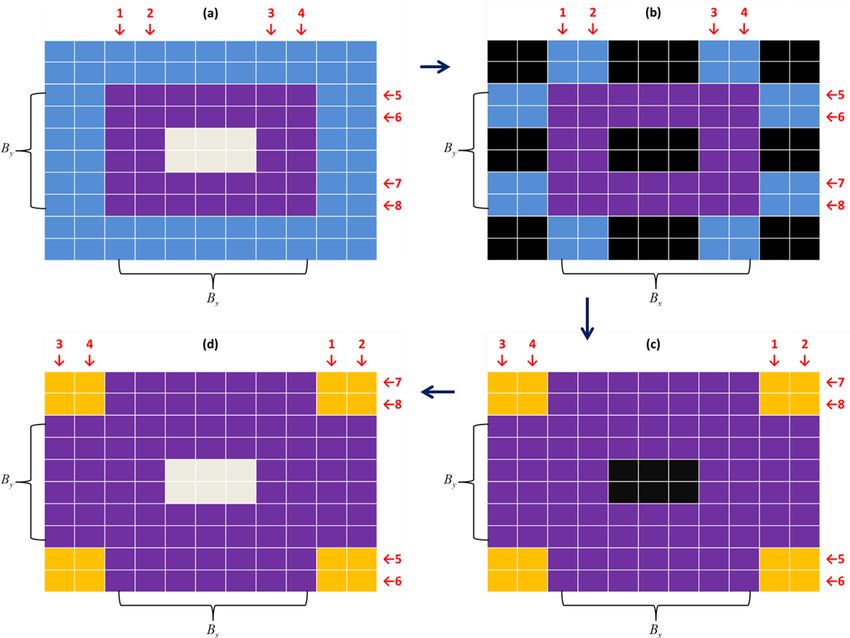
2790              P. Wang et al.: The GPU version of LICOM3 under the HIP framework and its large-scale application

Figure 7. The lateral packing (only transferring four rows and four columns of data between the GPU and CPU) method to accelerate the
halo. (a) In the GPU space, where central (gray) grids are unchanged; (b) transferred to the CPU space, where black grids mean no data;
(c) after halo with neighbors; and (d) transfer back to the GPU space.

   Figure 9 shows the roofline model using the Stream GPU             point operation performance is a little far from the oblique
and the LICOM program’s measured behavioral data on a                 roofline shown in Fig. 9. In particular, the subroutine bclinc
single computation node bound to one GPU card depict-                 apparently strays away from the entire trend for including
ing the relationship between arithmetic intensity and perfor-         frequent 3-D array Halo MPI communications, and much
mance floating point operations. The 100 km resolution case           data transmission occurs between the CPU and GPU.
is employed for the test. The blue and gray oblique lines                Figure 10 shows the SYPD at various parallel scales. The
are the fitting lines related to the Stream GPU program’s be-         baseline (384) of GPUs could achieve a 42 times faster
havioral data using 5.12 × 10⁸ and 1 × 10⁶ threads, respec-           speedup than that of the same number of CPU cores. Some-
tively, both with a block size of 256, which attain the best          times, we also count the overall speedup for 384 GPUs in 96
configuration. For details, the former is approximately the           nodes vs. the total 3072 CPU cores in 96 nodes. We can ob-
maximum thread number restricted by GPU card memory,                  tain an overall performance speedup of 384 or approximately
achieving a bandwidth limit of 696.52 GB s−1 . In compari-            6–7 times. The figure also indicates that for all scales, the
son, the latter is close to the average number of threads in          SYPD continues to increase. On the scale of 9216 GPUs, the
GPU parallel calculations used by LICOM, reaching a band-             SYPD first goes beyond 2, which is 7 times the same CPU
width of 344.87 GB s−1 on average. Here, we use the oblique           result. A quasi-whole-machine (26 200 GPUs, 26 200 × 65 =
gray line as a benchmark to verify the rationality of LI-             1 703 000 cores in total, one process corresponds to one CPU
COM’s performance, accomplishing an average bandwidth                 core plus 64 GPU cores) result indicates that it can still obtain
of 313.95 GB s−1 .                                                    an increasing SYPD to 2.72.
   Due to the large calculation scale of the entire LICOM                Since each node has 32 CPU cores and four GPUs, each
program, the divided calculation grid bound to a single GPU           GPU is managed by one CPU thread in the present cases.
card is limited by video memory; most kernel functions is-            We can also quantify GPUs’ speedup vs. all CPU cores on
sue no more than 1.2 × 10⁶ threads. As a result, the floating-        the same number of nodes. For example, 384 (768) GPUs

Geosci. Model Dev., 14, 2781–2799, 2021                                                https://doi.org/10.5194/gmd-14-2781-2021
P. Wang et al.: The GPU version of LICOM3 under the HIP framework and its large-scale application                                  2791

Figure 8. (a) The 384 GPUs and (b) 9216 GPUs, with the I/O ratio in total simulation time for the 1/20◦ setup, and (c) the changes in I/O
times vs. different GPUs.

                                                                       scale experiments for specific kernels. Our results are also
                                                                       slightly better than in Xu et al. (2015), who ported another
                                                                       ocean model to GPUs using Cuda C. However, due to the
                                                                       limitation of the number of Intel CPUs (maximum of 9216
                                                                       cores), we did not obtain the overall speedup for 1536 and
                                                                       more GPUs.
                                                                          Figure 11 depicts the actual times and speedups of dif-
                                                                       ferent GPU computations. The green line in Fig. 11a is a
                                                                       function of the stepon time cost; it decreases while the GPU
                                                                       number increases. The blue curve of Fig. 11a shows the in-
                                                                       crease in speedup with the rise in the GPU scale. Despite the
                                                                       speedup increase, the efficiency of the model decreases. At
                                                                       9216 GPUs, the model efficiency starts under 20 %, and for
                                                                       more GPUs (19 600 and 26 200), the efficiency is flattened
                                                                       to approximately 10 %. The efficiency decrease is mainly
                                                                       caused by the latency of the data copy in and out to the GPU
Figure 9. Roofline model for the AMD GPU and the performance           memory. For economic consideration, the 384–1536 scale is
of LICOM’s main subroutines.                                           a better choice for realistic modeling studies.
                                                                          Figure 12 depicts the time cost of seven core subroutines
                                                                       of LICOM3-HIP. We find that the top four most time-costly
correspond to 96 (192) nodes, which have 3072 (6144) CPU               subroutines are barotr, tracer, bclinc, and readyc, and the
cores. Therefore, the overall speedup is approximately 6.375           other subroutines cost only approximately 1 % of the whole
(0.51/0.08) for 384 GPUs and 4.15 (0.83/0.2) for 768 GPUs              computation time. When 384 GPUs are applied, the barotr
(Fig. 10). The speedups are comparable with our previous               costs approximately 50 % of the total time (Fig. 12a), which
work porting LICOM2 to GPU using OpenACC (Jiang et al.,                solves the barotropic equations. When GPUs are increased
2019), which is approximately 1.8–4.6 times the speedup us-            to 9216, each subroutine’s time cost decreases, but the per-
ing one GPU card vs. two eight-core Intel GPUs in small-               centage of subroutine barotr is increased to 62 % (Fig. 12b).

https://doi.org/10.5194/gmd-14-2781-2021                                                  Geosci. Model Dev., 14, 2781–2799, 2021
2792 P. Wang et al.: The GPU version of LICOM3 under the HIP framework and its large-scale application
Figure 10. Simulation performances of the AMD GPU vs. Intel CPU core for LICOM3 (1/20◦ ). Unit: SYPD.
Figure 11. (a) Computation time (green) and speedup (blue) and (b) parallel efficiency (orange) at different scales for stepons of LICOM3-
HIP (1/20◦ ).
As mentioned above, this phenomenon can be interpreted by gions near strong currents or high-latitude regions (Fig. 13c);
having more haloing in barotr than in the other subroutines; in most places, the difference in values fall into the range
hence, the memory data copy and communication latency of −0.1 and 0.1 cm. Because the hardware is different and
make it slower. the HIP codes’ mathematical operation sequence is not al-
ways the same as that for the Fortran version, the HIP and
4.2 Model performance in climate research CPU versions are not identical byte-by-byte. Therefore, it is
hard to verify the correctness of the results from the HIP ver-
sion. Usually, the ensemble method is employed to evaluate
The daily mean sea surface height (SSH) fields of the CPU
the consistency of two model runs (Baker et al., 2015). Con-
and HIP simulations are compared to test the usefulness of
sidering the unacceptable computing and storage resources,
the HIP version of LICOM for the numerical precision of
in addition to the differences between the two versions, we
scientific usage. Here, the results from 1/20◦ experiments
simply compute root mean square errors (RMSEs) between
on a particular day (1 March of the fourth model year) are
the two versions, which are only 0.18 cm, much smaller than
used (Fig. 13a and b). The general SSH spatial patterns of
the spatial variation of the system, which is 92 cm (approxi-
the two are visually very similar. Significant differences are
only found in very limited areas, such as in the eddy-rich re-
Geosci. Model Dev., 14, 2781–2799, 2021 https://doi.org/10.5194/gmd-14-2781-2021P. Wang et al.: The GPU version of LICOM3 under the HIP framework and its large-scale application 2793
Figure 12. The seven core subroutines’ time cost percentages for (a) 384 GPUs and (b) 9216 GPUs. (c) The subroutines’ time cost at different
scales of LICOM3-HIP (1/20◦ ).
mately 0.2 %). This indicates that the results of LICO3-HIP these mesoscale eddies must be solved in the ocean model.
are generally acceptable for research. A numerical model’s horizontal resolution must be higher
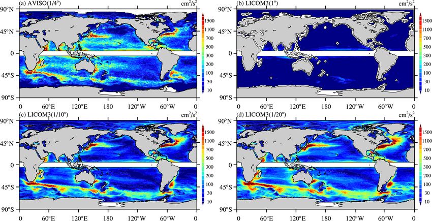
The GPU version’s sea surface temperature (SST) is than 1/10◦ to resolve the global ocean eddies but cannot re-
compared with the observed SST to evaluate the global solve the eddies in high-latitude and shallow waters (Hall-
1/20◦ simulation’s preliminary results from LICOM3-HIP berg, 2013). Therefore, a higher resolution is required to de-
(Fig. 14). Because the LICOM3-HIP experiments are forced termine the eddies globally. The EKE for the 1◦ version is
by the daily mean atmospheric variables in 2016, we also low, even in the areas with strong currents, while the 1/10◦
compare the outputs with the observation data in 2016. Here, version can reproduce most of the eddy-rich regions in the
the 1/4◦ Optimum Interpolation Sea Surface Temperature observation. The EKE increases when the resolution is fur-
(OISST) is employed for comparison, and the simulated SST ther enhanced to 1/20◦ , indicating that many more eddy ac-
is interpolated to the same resolution as the OISST. We find tivities are resolved.
that the global mean values of SST are close together but
with a slight warming bias of 18.49 ◦ C for observations vs.
18.96 ◦ C for the model. The spatial pattern of SST in 2016 is
well reproduced by LICOM3-HIP. The spatial standard de- 5 Discussion
viation (SD) of SST is 11.55 ◦ C for OISST and 10.98 ◦ C for
LICOM3-HIP. The RMSE of LICOM3-HIP against the ob- 5.1 Application of the ocean climate model beyond
servation is only 0.84 ◦ C. 10 000 GPUs
With an increasing horizontal resolution of the observa-
tions, we now know that mesoscale eddies are ubiquitous in Table 4 summarizes the detailed features of some published
the ocean at the 100–300 km spatial scale. Rigorous eddies GPU version models. We find that various programming
usually occur along significant ocean currents, such as the methods have been implemented for different models. A
Kuroshio and its extension, the Gulf Stream, and the Antarc- near-kilometer atmospheric model using 4888 GPUs was re-
tic Circumpolar Current (Fig. 15a). Eddies also capture more ported as a large-scale example of weather/climate studies.
than 80 % of the ocean’s kinetic energy, which was estimated With supercomputing development, the horizontal resolu-
using satellite data (e.g., Chelton et al., 2011). Therefore, tion of ocean circulation models will keep increasing, and
more sophisticated physical processes will also be devel-
https://doi.org/10.5194/gmd-14-2781-2021 Geosci. Model Dev., 14, 2781–2799, 20212794 P. Wang et al.: The GPU version of LICOM3 under the HIP framework and its large-scale application
Figure 14. (a) Observed annual mean sea surface temperature in
2016 from the Optimum Interpolation Sea Surface Temperature
(OISST); (b) simulated annual mean SST for LICOM3-HIP at
1/20◦ during model years 0005–0014. Units: ◦ C.
in 100 000 h). As the MPI (GPU) scale increases, the total
error rate increases, and once a hardware error occurs, the
model simulation will fail.
When 384 GPUs are applied, the success rate within 1 h
Figure 13. Daily mean simulated sea surface height for (a) CPU can be expressed as (1 − 384 × 10−5 )3 = 98.85 %, and the
and (b) HIP versions of LICOM3 at 1/20◦ on 1 March of the fourth failure rate is then 1 − (1 − 384 × 10−5 )3 = 1.15 %. Apply-
model year. (c) The difference between the two versions (HIP minus ing this formula, we can obtain the failure rate correspond-
CPU). Units: cm. ing to 1000, 10 000, and 26 200 GPUs. The results are listed
in Table 5. As shown in Table 5, on the medium scale
(i.e., 1000 GPUs are used), three failures will occur through
oped. LICOM3-HIP has a larger scale, not only in terms of 100 runs; when the scale increases to 10 000 GPUs, one-
grid size but also in final GPU numbers. quarter of them will fail. The 10−5 error probability also indi-
We successfully performed a quasi-whole-machine cates that 10 000 GPU tasks cannot run 10 continuous hours
(26 200 GPUs) test, and the results indicate that the model on average. If the success time restriction decreases, the
obtained an increasing SYPD (2.72). The application of model success rate will increase. For example, within 6 min,
an ocean climate model beyond 10 000 GPUs is not easy the 26 200 GPU task success rate is (1 − 26 200 × 10−6 )3 =
because running the multi-nodes plus multi-GPUs requires 9234 %, and its failure rate is 1 − (1 − 26 200 × 10−6 )3 =
that the network connection, PCI-e and memory speed, 7.66 %.
and input/output storage systems all work to their best
performances. Gupta et al. (2017) investigated 23 types 5.2 Energy to solution
of system failures to improve the reliability of the HPC
We also measured the energy to solution here. A simulation-
(high-performance computing) system. Unlike in Gupta’s
normalized energy (E) is employed here as a metric. The
study, only the three most common types of failures we
formula is as follows:
encountered are discussed here. The three most common
errors when running LICOM3-HIP are MPI hardware errors, E = TDP × N × 24/SYPD,
CPU memory access errors, and GPU hardware errors. Let
us suppose that the probability of an individual hardware (or where TDP is the thermal design power, N is the computer
software) error occurring is 10−5 (which means one failure nodes used, and SYPD/24 equals the simulated years per
Geosci. Model Dev., 14, 2781–2799, 2021 https://doi.org/10.5194/gmd-14-2781-2021P. Wang et al.: The GPU version of LICOM3 under the HIP framework and its large-scale application 2795
Figure 15. (a) Observed annual mean eddy kinetic energy (EKE) in 2016 from AVISO (Archiving, Validation and Interpretation of Satellite
Oceanographic). Simulated annual mean SST in 2016 for LICOM3-HIP at (b) 1◦ , (c) 1/10◦ , and (d) 1/20◦ . Units: cm2 s−2 .
Table 4. Some GPU versions of weather/climate models.
Model Language Max. grids Max GPUs Year and references
POM.gpu CUDA-C 1922 × 1442 × 51 4 (K20X) 2015 (Xu et al., 2015)
LICOM2 OpenACC 360 × 218 × 30 4 (K80) 2019 (Jiang et al., 2019)
FUNWAVE CUDA-Fortran 3200 × 2400 2 (V100) 2020 (Yuan et al., 2020)
NICAM OpenACC 56 × 56 km×160 2560 (K20X) 2016 (Yashiro et al., 2016)
COSMO OpenACC 346 × 340 × 60 4888 (P100) 2018 (Fuhrer et al., 2018)
LICOM3 HIP 7200 × 3920 × 55 26 200 (gfx906) 2020 (This paper)
Table 5. Success and failure rates of different scales for 1 wall clock simulation year (MWh SY−1 ). The energy costs for the
hour simulation. 1/20◦ LICOM3 simulations running on CPUs and GPUs
are comparable when the numbers of MPI processors are
GPUs Success Failure within 1000. The energy costs of LICOM3 at 1/20◦ run-
384 98.85 % 1.15 % ning on 384 (768) GPUs and CPUs are approximately 6.234
1000 97.02 % 2.98 % (7.661) MWh SY−1 and 6.845 (6.280) MWh SY−1 , respec-
10 000 72.90 % 27.10 % tively. However, the simulation speed of LICOM3 on a GPU
26 200 40.19 % 59.81 % is much faster than that on a CPU: approximately 42 times
faster for 384 processors and 31 times faster for 768 proces-
sors. When the number of MPI processors is beyond 1000,
hour. Therefore, the smaller the E value is, the better, which the value of E for the GPU becomes much larger than that
means that we can obtain more simulated years within a lim- for the CPU. This result indicates that the GPU is not fully
ited power supply. To calculate E’s value, we estimated the loaded at this scale.
TDP of 1380 W for a node on the present platform (one AMD
CPU and four GPUs) and 290 W for a reference node (two
Intel 16-core CPUs). We only include the TDP of CPUs and 6 Conclusions
GPUs here.
Based on the above power measurements, the simu- The GPU version of LICOM3 under the HIP framework was
lations’ energy cost is calculated in megawatt-hours per developed in the present study. Seven kernels within the time
https://doi.org/10.5194/gmd-14-2781-2021 Geosci. Model Dev., 14, 2781–2799, 20212796 P. Wang et al.: The GPU version of LICOM3 under the HIP framework and its large-scale application
integration of the mode are all ported to the GPU, and 3-D the original in the spin-up simulation, the performance will
parallelization (also partitioned in the vertical direction) is achieve 1–2.5 SYPD for 384–1536 GPUs. This performance
applied. The new model was implemented and gained an ex- will satisfy 10–50-year-scale climate studies. In addition, this
cellent acceleration rate on a Linux cluster with AMD GPU version can be used for short-term ocean prediction in the fu-
cards. This is also the first time an ocean general circulation ture.
model has been fully applied on a heterogeneous supercom- Additionally, the block size of 36 × 30 × 55 (1/20◦ setup,
puter using the HIP framework. In total, it took 19 months, 26 200 GPUs) is not an enormous computational task for
five PhD students and five part-time staff to finish the porting one GPU. Since one GPU has 64 cores and a total of
and testing work. 2560 threads, if a subroutine computation is 2-D, each
Based on our test using the 1/20◦ configuration, LICOM3- thread’s operation is too small. Even for the 3-D loops, it is
HIP is 42 times faster than the CPU when 384 AMD GPUs still not large enough to load the entire GPU. This indicates
and CPU cores are used. LICOM3-HIP has good scalability, that it will gain more speedup when the LICOM resolution
and can obtain a speedup of more than 4 on 9216 GPUs com- is increased to the kilometer level. The LICOM3-HIP codes
pared to 384 GPUs. The SYPD, which is in equilibrium with are now written for 1/20◦ , but they are kilometer-ready GPU
the speedup, continues to increase as the number of GPUs in- codes.
creases. We successfully performed a quasi-whole-machine The optimization strategies here are mostly at the program
test, which was 6550 nodes and 26 200 GPUs, using 1/20◦ level and do not treat the dynamic or physics parts separately.
LICOM3-HIP on the supercomputer, and at the grand scale, We only ported all seven core subroutines to the GPU to-
the model can obtain an increasing SYPD of 2.72. The mod- gether, i.e., including both the dynamic and physics parts,
ification or optimization of the model also improves the 10 within the time integration loops. Unlike atmospheric mod-
and 100 km performances, although we did not analyze their els, there are a few time-consuming physical processes in
performances in this article. ocean models, such as radiative transportation, clouds, pre-
The efficiency of the model decreases with the increas- cipitation, and convection processes. Therefore, the two parts
ing number of GPUs. At 9216 GPUs, the model efficiency are usually not separated in the ocean model, particularly in
starts under 20 % against 384 GPUs, and when the number the early stage of model development. This is also the case
of GPUs reaches or exceeds 20 000, the efficiency is only ap- for LICOM. Further optimization to explicitly separate the
proximately 10 %. Based on our kernel function test, the de- dynamic core and the physical package is necessary in the
creasing efficiency was mainly caused by the latency of data future.
copy in and out to the GPU memory in solving the barotropic There is still potential to further increase the speedup of
equations, particularly for the number of GPUs larger than LICOM3-HIP. The bottleneck is in the high-frequency data
10 000. copy in and out to the GPU memory in the barotropic part
Using the 1/20◦ configuration of LICOM3-HIP, we con- of LICOM3. Unless HIP-aware MPI is supported, the data
ducted a 14-year spin-up integration. Because the hardware transfer latency between the CPU and GPU cannot be over-
is different and the GPU codes’ mathematical operation se- come. Thus far, we can only reduce the time consumed by
quence is not always the same as that of the Fortran version, decreasing the frequency or magnitude of the data copy and
the GPU and CPU versions cannot be identical byte by byte. even modifying the method to solve the barotropic equations.
The comparison between the GPU and CPU versions of LI- Additionally, using single precision within the time integra-
COM3 shows that the differences are minimal in most places, tion of LICOM3 might be another solution. The mixing-
indicating that the results from LICOM3-HIP can be used precision method has already been tested using an atmo-
for practical research. Further comparison with the observa- spheric model, and the average gain in computational effi-
tion and the lower-resolution results suggests that the 1/20◦ ciency is approximately 40 % (Váňa et al., 2017). We would
configuration of LICOM3-HIP can reproduce the observed like to try these methods in the future.
large-scale features and produce much smaller-scale activi-
ties than that of lower-resolution results.
The eddy-resolving ocean circulation model, which is a Code availability. The model code (LICOM3-HIP V1.0) along
virtual platform for oceanography research, ocean forecast- with the dataset and a 100 km case can be downloaded from
ing, and climate prediction and projection, can simulate the the website https://zenodo.org/record/4302813# (last access: 3 De-
variations in circulations, temperature, salinity, and sea level cember 2020). X8 mGWcsvNb8 has the following digital object
identifier (doi): https://doi.org/10.5281/zenodo.4302813 (Liu et al.,
with a spatial scale larger than 15 km and a temporal scale
2020).
from the diurnal cycle to decadal variability. As mentioned
above, 1–2 SYPD is a good start for a realistic climate re-
search model. The more practical GPU scale range for a re- Data availability. The data for figures in this paper can be
alistic simulation is approximately 384–1536 GPUs. At these downloaded from https://zenodo.org/record/4542544# (last ac-
scales, the model still has 0.5–1.22 SYPD. Even if we de-
crease the loops in the barotr procedure to one-third of
Geosci. Model Dev., 14, 2781–2799, 2021 https://doi.org/10.5194/gmd-14-2781-2021You can also read