GTS v1.0: a macrophysics scheme for climate models based on a probability density function
←
→
Page content transcription
If your browser does not render page correctly, please read the page content below
Geosci. Model Dev., 14, 177–204, 2021
https://doi.org/10.5194/gmd-14-177-2021
© Author(s) 2021. This work is distributed under
the Creative Commons Attribution 4.0 License.

GTS v1.0: a macrophysics scheme for climate models based on a
probability density function
Chein-Jung Shiu1 , Yi-Chi Wang1 , Huang-Hsiung Hsu1 , Wei-Ting Chen2 , Hua-Lu Pan3 , Ruiyu Sun4 , Yi-Hsuan Chen5 ,
and Cheng-An Chen1
1 Research Center for Environmental Changes, Academia Sinica, Taipei, Taiwan
2 Department  of Atmospheric Sciences, National Taiwan University, Taipei, Taiwan
3 Retired Senior Scientist, National Centers for Environmental Prediction, NOAA, College Park, Maryland, USA
4 National Centers for Environmental Prediction, NOAA, College Park, Maryland, USA
5 Department of Climate and Space Sciences and Engineering, University of Michigan, Ann Arbor, Michigan, USA

Correspondence: Chein-Jung Shiu (cjshiu@rcec.sinica.edu.tw)

Received: 15 May 2020 – Discussion started: 7 July 2020
Revised: 16 November 2020 – Accepted: 17 November 2020 – Published: 12 January 2021

Abstract. Cloud macrophysics schemes are unique param-           variables are improved compared with the default scheme,
eterizations for general circulation models. We propose an       particularly with respect to water vapor and RH fields. Dif-
approach based on a probability density function (PDF) that      ferent PDF shapes in the GTS scheme also significantly af-
utilizes cloud condensates and saturation ratios to replace      fect global simulations.
the assumption of critical relative humidity (RH). We test
this approach, called the Global Forecast System (GFS) –
Taiwan Earth System Model (TaiESM) – Sundqvist (GTS)
scheme, using the macrophysics scheme within the Commu-          1   Introduction
nity Atmosphere Model version 5.3 (CAM5.3) framework.
Via single-column model results, the new approach simu-          Global weather and climate models commonly use cloud
lates the cloud fraction (CF)–RH distributions closer to those   macrophysics parameterization to calculate the subgrid cloud
of the observations when compared to those of the default        fraction (CF) and/or large-scale cloud condensate, as well as
CAM5.3 scheme. We also validate the impact of the GTS            cloud overlap, which is required in cloud microphysics and
scheme on global climate simulations with satellite observa-     radiation schemes (Slingo, 1987; Sundqvist, 1988; Sundqvist
tions. The simulated CF is comparable to CloudSat/Cloud-         et al., 1989; Smith, 1990; Tiedtke, 1993; Xu and Randall,
Aerosol Lidar and Infrared Pathfinder Satellite Observation      1996; Rasch and Kristjansson, 1998; Jakob and Klein, 2000;
(CALIPSO) data. Comparisons of the vertical distributions        Tompkins, 2002; Zhang et al., 2003; Wilson et al., 2008a,
of CF and cloud water content (CWC), as functions of             b; Chabourea and Bechtold, 2002; Park et al., 2014, 2016).
large-scale dynamic and thermodynamic parameters, with           The largest uncertainty in climate prediction is associated
the CloudSat/CALIPSO data suggest that the GTS scheme            with clouds and aerosols (Boucher et al., 2013). The large
can closely simulate observations. This is particularly no-      number of cloud-related parameterizations in general circu-
ticeable for thermodynamic parameters, such as RH, upper-        lation models (GCMs) contributes to this uncertainty. In re-
tropospheric temperature, and total precipitable water, im-      cent years, an increasing amount of research has been de-
plying that our scheme can simulate variation in CF associ-      voted to unifying cloud-related parameterizations, for exam-
ated with RH more reliably than the default scheme. Changes      ple, by incorporating the planetary boundary layer, shallow
in CF and CWC would affect climatic fields and large-scale       and/or deep convection, and stratiform cloud (cloud macro-
circulation via cloud–radiation interaction. Both climatolog-    physics and/or microphysics) parameterizations, to improve
ical means and annual cycles of many of the GTS-simulated        cloud simulations in large-scale global models (Bogenschutz
                                                                 et al., 2013; Park et al., 2014a, b; Storer et al., 2015).

Published by Copernicus Publications on behalf of the European Geosciences Union.
178                                                                        C.-J. Shiu et al.: Macrophysics for climate models

   Some of these parameterizations use prognostic ap-              Academia Sinica. Park et al. (2014) discussed a similar ap-
proaches to parameterize the CF (Tiedtke, 1993; Tompkins,          proach wherein a triangular PDF was used to diagnose cloud
2002; Wilson et al., 2008a, b; Park et al., 2016), while oth-      liquid water as well as the liquid cloud fraction, and sug-
ers use diagnostic approaches (Sundqvist et al., 1989; Smith,      gested that the PDF width could be computed internally
1990; Xu and Randall, 1996; Zhang et al., 2003; Park et            rather than specified, to consistently diagnose both CF and
al., 2014). Most of the diagnostic approaches used in GCM          cloud liquid water as in macrophysics. These authors also
cloud macrophysical schemes use the critical relative humid-       mentioned that such stratus cloud macrophysics could be ap-
ity threshold (RHc ) to calculate CF (Slingo, 1987; Sundqvist      plied across any horizontal and vertical resolution of a GCM
et al., 1989; Roeckner et al., 1996). In this type of parame-      grid, although they did not formally implement and test this
terization, GCMs frequently use the RHc value as a tunable         idea using their scheme. Building upon their ideas, we im-
parameter (Mauritsen et al., 2012; Golaz et al., 2013; Hour-       plemented and tested this assumption with a triangular PDF
din et al., 2017). There are some studies on the verification      in the GTS scheme.
of global simulations focused on the cloud macrophysical              In summary, this GTS scheme adopts Sundqvist’s assump-
parameterization (Hogan et al., 2009; Franklin et al., 2012;       tion regarding the partition of cloudy and clear regions within
Qian et al., 2012; Sotiropoulou et al., 2015). In addition,        a model grid box but uses a variable PDF width once clouds
many model development studies show the impact of total            are formed. It introduces a self-consistent diagnostic calcu-
water used in CF schemes on global simulations after modi-         lation of CF. Due to their use of an internally computed PDF
fying the RHc and/or the probability density function (PDF)        width, GTS schemes are expected to be able to better repre-
(Donner et al., 2011; Neale et al., 2013; Schmidt et al., 2014).   sent the relative variation of CF with RH in GCM grids.
Some recent studies have attempted to constrain RHc from              A variety of assumptions regarding PDF shape can be
regional sounding observations and/or satellite retrievals to      adopted in diagnostic approaches (Sommeria and Deardorff,
improve regional and/or global simulations (Quaas, 2012;           1977; Bougeault, 1982; Smith, 1990; Tompkins, 2002).
Molod, 2012; Lin, 2014).                                           Some studies have investigated representing cloud conden-
   While many variations of the diagnostic Sundqvist CF            sate and water vapor in a more statistically accurate way
scheme have been proposed, most numerical weather predic-          by using more complex types of PDF to represent param-
tion models and GCMs use the basic principle proposed by           eters such as total water, CF, and updraft vertical velocity
Sundqvist et al. (1989): the changes in cloud condensate in        (Larson, 2002; Golaz et al., 2002; Firl, 2013; Bogenschutz
a grid box are derived from the budget equation for RH. In         et al., 2012; Bogenschutz and Krueger, 2013; Firl and Ran-
the meantime, the amount of additional moisture from other         dall, 2015). In this study, we apply and investigate two simple
processes is divided between the cloudy portion and the clear      and commonly used PDF shapes – uniform and triangular –
portion according to the proportion of clouds determined us-       in our parameterization of the GTS macrophysics scheme.
ing an assumed RHc . While changes have been made to other         Other complex types of PDF assumptions can also be used
parts of the Sundqvist scheme, the CF–RHc relationship still       if analytical solutions regarding the width of the PDF can be
applies in most Sundqvist-based schemes. As highlighted by         derived.
Tompkins (2005), the RHc value in the Sundqvist scheme                Most of the studies mentioned above estimate the CF via
can be related to the assumption of uniform distribution for       cloud liquid or total cloud water. Earlier versions of GCMs
the total water in an unsaturated grid box such that the dis-      used a Slingo-type approach to resolve the ice cloud frac-
tribution width (δc ) of the situation when a cloud is about to    tion (Slingo, 1987; Tompkins et al., 2007; Park et al., 2014).
form is given by                                                   On the other hand, the current generation of global models
                                                                   participating in the Coupled Model Intercomparison Project
δc = qs (1 − RHc ) ,                                        (1)
                                                                   phase 6 (CMIP6) have alternative approaches for the han-
where qs is the saturated mixing ratio.                            dling of CFs associated with ice clouds. In the GTS scheme,
   We re-derived this equation by describing the change in         the approach to cloud liquid water fraction parameterization
the distribution width δ with grid-mean cloud condensates          is extended to the ice cloud fraction as well, wherein the sat-
and saturation ratio using the basic assumption of uniform         uration mixing ratio (qs ) with respect to water is replaced by
distribution from Sundqvist et al. (1989) rather than using        qs with respect to ice. This provides a consistent treatment for
the RHc -derived δc , thereby eliminating unnecessary use of       the liquid cloud and ice cloud fractions. Many studies have
the RHc while retaining the PDF assumption for the entire          argued that the assumption of rapid adjustment between wa-
scheme. This modified macrophysics scheme is named the             ter vapor and cloud liquid water applied in GCM CF schemes
GFS–TaiESM–Sundqvist (GTS) scheme version 1.0 (GTS                 cannot be applied to ice clouds (Tompkins et al., 2007; Salz-
v1.0). It was first developed for the Global Forecast Sys-         mann et al., 2010; Chosson et al., 2014). In addition, it would
tem (GFS) model at the National Centers for Environmen-            be difficult to represent the CF of mixed-phase clouds using
tal Prediction (NCEP) and has been further improved for the        such an assumption (McCoy et al., 2016). Applying a diag-
Taiwan Earth System Model (TaiESM; Lee et al., 2020a)              nostic approach to the ice cloud fraction similar to that used
at the Research Center for Environmental Changes (RCEC),           for the liquid cloud fraction is indeed challenging and may

Geosci. Model Dev., 14, 177–204, 2021                                                https://doi.org/10.5194/gmd-14-177-2021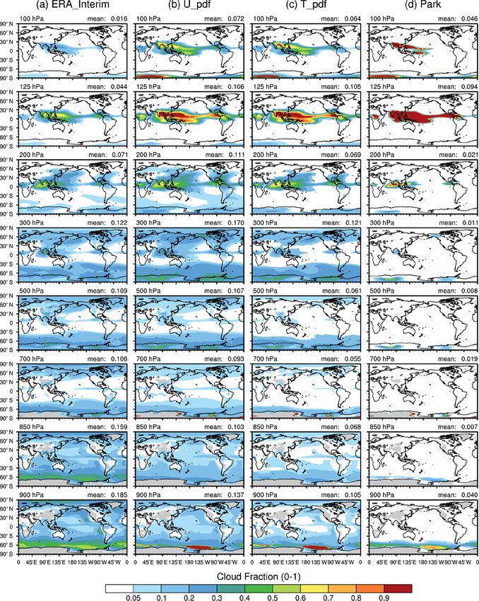
C.-J. Shiu et al.: Macrophysics for climate models                                                                                 179

                                                                       P (qt ) with information about qv and ql provided by the base
                                                                       model. Please note that uniform temperature is assumed over
                                                                       the grid for the GTS scheme.
                                                                          With uniform PDF as denoted in Fig. 1a, the liquid cloud
                                                                       fraction (bl ) and grid-mean cloud liquid mixing ratio (ql ) can
                                                                       be integrated as follows:
                                                                           Z∞
                                                                                          1
                                                                       bl = P (qt ) dqt =    (ql + qv + δ − qs ) ,                 (4)
                                                                                          2δ
                                                                              qs

                                                                       and
Figure 1. Illustration of subgrid PDF of total water substance qt          Z∞
                                                                                                    1
with (a) uniform distribution and (b) triangular distribution. The     ql = (qt − qs )P (qt ) dqt =    q t + δ − qs .              (5)
shaded part shows the saturated cloud fraction, δ represents the                                    4δ
                                                                              qs
width of the PDF, qt denotes the grid-mean value of total water
substance, and qs represents the saturation mixing ratio as the tem-   Given ql , qv , and qs , the width of uniform PDF can be deter-
perature is assumed to be uniform within the grid. Please note that    mined as follows:
uniform temperature assumption is used for the GTS cloud macro-            p        p           2
physics.                                                               δ=     ql + qs − qv .                                       (6)

                                                                       Therefore, we can calculate the liquid cloud fraction from
result in a high level of uncertainty. To investigate this is-         Eq. (4).
sue, we also conduct a series of sensitivity tests related to             In addition to the application of a PDF-based approach for
the supersaturation ratio assumption, which is applied when            liquid CF parameterization, the GTS scheme also uses the
calculating the ice cloud fraction in the GTS scheme.                  same concept for parameterizing the ice CF (bi ) as follows:
                                                                              1
                                                                       bi =      (q + q v + δ − sup · qsi ),                       (7)
2     Descriptions of scheme, model, and simulation setup                    2δ i
                                                                       where q i , q v , and qsi denote the grid-mean cloud ice mixing
2.1    Scheme descriptions
                                                                       ratio, water vapor mixing ratio, and saturation mixing ratio
Figure 1 illustrates the PDF-based scheme with a uniform               over ice, respectively. In Eq. (7), qsi is multiplied by a su-
PDF and a triangular PDF of total water substance qt . By as-          persaturation factor (“sup”) to account for the situation in
suming that the clear region is free of condensates and that           which rapid saturation adjustment is not reached for cloud
the cloudy region is fully saturated, the cloudy region (b) be-        ice. In the present version of the GTS scheme, sup is tem-
comes the area where qt is larger than the saturation value qs         porarily assumed to be 1.0. Sensitivity tests regarding sup
(shaded area). The PDF-based scheme automatically retains              will be discussed in Sect. 5.6. Values of qi and qv used to
consistency between CF and condensates because it is de-               calculate Eq. (7) are the updated state variables before call-
rived from the same PDF. Here, we used the uniform PDF to              ing the cloud macrophysics process.
demonstrate the relationship between RHc and the width of                 A more complex PDF can be used for P (qt ) instead
the PDF. Using a derivation extended from Tompkins (2005),             of the uniform distribution in our derivation. For example,
                                                                       the Community Atmosphere Model version 5.3 (CAM5.3)
      1                                                                macrophysics model adopts a triangular PDF instead of a
b=       (qt + δ − qs ).                                        (2)
      2δ                                                               uniform PDF to represent the subgrid distribution of the to-
It is evident that, with the uniform PDF,                              tal water substance (Park et al., 2014). Mathematically, the
                                                                       triangular distribution is a more accurate approximation of
δc = qs (1 − RHc ) .                                            (3)    the Gaussian distribution than the uniform distribution and it
                                                                       may also be more realistic. Therefore, we followed the same
Therefore, RHc = 1 − qδcs . Thus, if the width δ of the uni-
                                                                       procedure to diagnose the CF by forming a triangular PDF
form PDF is determined, then RHc can be determined ac-
                                                                       with ql , qv , and qs provided. Moreover, by using a triangular
cordingly. This relation reveals that the RHc assumption of
                                                                       PDF, we can obtain results that are more comparable to the
the RH-based scheme actually assumes the width of the uni-
                                                                       CAM5.3 macrophysics scheme because the same PDF was
form PDF to be δc from the PDF-based scheme. As noticed
                                                                       used. By considering the PDF width, the CF (b) and liquid
by Tompkins (2005), the RHc used by Sundqvist et al. (1989)
                                                                       water content (ql ) can be written as follows:
for cloud generation can be linked to the statistical cloud                  1
scheme with a uniform distribution. Building upon this find-                      (1 − s )2        if ss > 0
                                                                       b= 2 1 s                2              ,                    (8)
ing, we eliminated the assumption of RHc by determining the                     1 − 2 (1 + ss ) if ss < 0

https://doi.org/10.5194/gmd-14-177-2021                                                     Geosci. Model Dev., 14, 177–204, 2021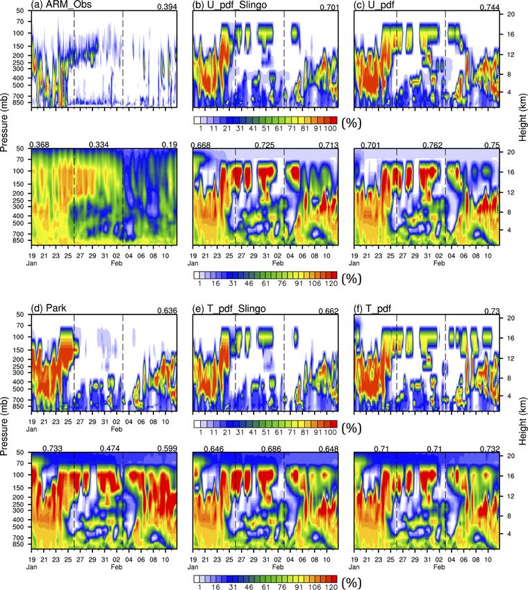
180                                                                       C.-J. Shiu et al.: Macrophysics for climate models

and                                                              the responses of physical schemes under environmental forc-
       (                                                         ing of different regimes of interest. Here, we adopt the case
ql         1       ss2       ss3
               −         − ss b
                         +                if   ss > 0 ,          of Tropical Warm Pool – International Cloud Experiment
   =       6        6         6                            (9)
δ          − 61 − 16 3ss2 − 2ss3 − ss b   if   ss < 0            (TWP-ICE), which was supported by the ARM program of
                                                                 the Department of Energy and the Bureau of Meteorology
respectively, where ss = qs −q  t                                of Australia from January to February 2006 over Darwin in
                              δ . From these two equations,
we can derive the width of the triangular PDF and calcu-         northern Australia. Based on the meteorological conditions,
late the CF (b) based on qs , qt , and qv instead of RHc . De-   the TWP-ICE period can be divided into four shorter periods:
tailed derivations of Eqs. (8) and (9) can be seen in Ap-        the active monsoon period (19–25 January), the suppressed
pendix A. Notably, the PDF width for the total water sub-        monsoon period (26 January to 2 February), the monsoon
stance can only be constrained when the cloud exists. There-     clear-sky period (3–5 February), and the monsoon break pe-
fore, the RHc is still required when clouds start to form from   riod (6–13 February; May et al., 2008; Xie et al., 2010). To
a clear region. To simplify the cloud macrophysics param-        take advantage of previous studies of cloud-resolving models
eterization, value of RHc in the GTS scheme is assumed           and single-column models, we followed the setup of Franklin
to be 0.8 instead of RHc varying with height in the default      et al. (2012) to initiate the single-column runs starting on
Park scheme. The GTS scheme still uses the default prog-         19 January 2006 and running for 25 d.
nostic scheme for calculating cloud condensates (Park et al.,       Stand-alone CAM5.3 simulations of the CESM model,
2014), and it has effects only on the stratiform CFs. Although   forced by climatological sea surface temperature for the
the GTS scheme is presumed to have good consistency be-          year 2000 (i.e., CESM compset: F_2000_CAM5), are con-
tween CF and condensates, the consistency check subrou-          ducted to demonstrate global results. The horizontal resolu-
tines of the Park scheme are still kept in the GTS scheme to     tion of the CESM global runs is set at 2◦ . Individual global
avoid “empty” and “dense” clouds due to the usage of the         simulations are integrated for 12 years, and the output for the
Park scheme for calculating cloud condensates, and the GTS       last 10 years is used to calculate climatological means and
schemes still need RHc when clouds start to form.                annual cycles in global means. Because we made changes
   In this study, GTS schemes utilizing two different PDF        largely with respect to CF, we also conducted correspond-
shape assumptions are evaluated: uniform (hereafter, U_pdf)      ing simulations using the satellite-simulator approach to pro-
and triangular (hereafter, T_pdf). These two PDF types are       vide CF for a fair comparison with satellite CF products and
specifically formulated to evaluate the effects of the choice    typical CESM model output. This was done using the Cloud
of PDF shape. A triangular PDF is the default shape used         Feedback Model Intercomparison Project (CFMIP) Observa-
for cloud macrophysics by CAM5.3 (hereafter, the Park            tion Simulator Package (COSP) built into CESM 1.2.2 (Kay
scheme). The T_pdf of the GTS scheme is numerically sim-         et al., 2012). In addition to the default monthly outputs, daily
ilar to that of the Park scheme except for using a variable      outputs of several selected variables are also written out for
width for the triangular PDF once clouds are formed.             more in-depth analysis.

2.2    Model description and simulation setup
                                                                 3     Observational datasets and offline calculations
The GTS schemes described in this study were implemented
into CAM5.3 in the Community Earth System Model ver-             3.1    Observational data
sion 1.2.2 (CESM 1.2.2), which is developed and main-
tained by Department of Energy (DOE) University Corpo-           Cloud field comparisons are critical for modifications to our
ration for Atmospheric Research/National Center for At-          system with respect to cloud macrophysical schemes. There-
mospheric Research (UCAR/NCAR). Physical parameteri-             fore, we use the products from CloudSat/Cloud-Aerosol Li-
zations of CAM5.3 include deep convection, shallow con-          dar and Infrared Pathfinder Satellite Observation (CALIPSO)
vection, macrophysics, aerosol activation, stratiform micro-     to provide CF data for evaluating the modeling capabilities of
physics, wet deposition of aerosols, radiation, a chemistry      the default and modified GTS cloud macrophysical schemes.
and aerosol module, moist turbulence, dry deposition of          This dataset (provided by the AMWG diagnostics package of
aerosols, and dynamics. References for the individual phys-      NCAR) is used to compare with CF simulated by the COSP
ical parameterizations can be found in the NCAR technical        satellite simulator of CESM 1.2.2. Notably, this dataset is
notes (Neale et al., 2010). The master equations are solved on   different from the one below which also includes cloud wa-
a vertical hybrid pressure–sigma coordinate system (30 ver-      ter content (CWC).
tical levels) using the finite-volume dynamical core option of      In addition to cloud observations, observational radiation
CAM5.3.                                                          fluxes from the Clouds and the Earth’s Radiant Energy
   We conducted both the single-column tests and stand-          System – Energy Balanced and Filled (EBAF) product
alone global-domain simulations with CAM5.3 physics. The         (CERES-EBAF) are also used to investigate whether simu-
single-column setup provides the benefit of understanding        lations using our system will improve radiation calculations

Geosci. Model Dev., 14, 177–204, 2021                                              https://doi.org/10.5194/gmd-14-177-2021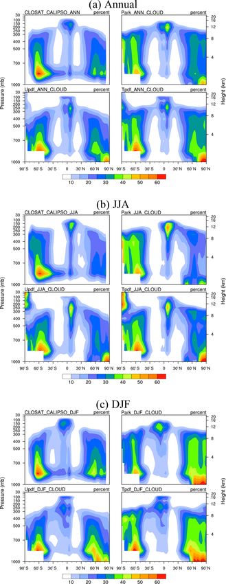
C.-J. Shiu et al.: Macrophysics for climate models                                                                             181

for both shortwave and longwave radiation flux, as well as         ing Eqs. (6) and (4) when ql is greater than 10−10 (kg kg−1 ).
their corresponding cloud radiative forcings. Precipitation        When ql is smaller than 10−10 (kg kg−1 ) and if RH > RHc ,
data are compared with Global Precipitation Climatology            CFs are calculated based on Eq. (3) and the liquid CF param-
Project data and several other climatic parameters, e.g.,          eterization of Sundqvist et al. (1989), and if RH < RHc , CFs
air temperature, RH, precipitable water, and zonal wind,           are equal to zero. Ice CFs are calculated similarly to those of
are evaluated against the reanalysis data (ERA-Interim).           liquid CFs but using Eq. (7), q i , q si , and sup of 1.0. Proce-
All these observational data are also obtained from the            dures for calculating CFs diagnosed by the T_pdf of the GTS
AMWG diagnostics package provided by NCAR and their                scheme are similar to those of U_pdf but using the equation
corresponding datasets can be found in the NCAR Climate            set of the triangular PDF. Values of RHc used in the U_pdf
Data Guide (https://climatedataguide.ucar.edu/collections/         and T_pdf of GTS schemes are assumed to be 0.8 and height
diagnostic-data-sets/ncar-doe-cesm/atmosdiagnostics, last          independent. The maximum overlapping assumption is used
access: 8 January 2021). The time periods used to calculate        to calculate the horizontal overlap between the liquid CF and
the climatological means are simply following the default          ice CF.
setup of the AMWG diagnostics package.                                Overall, the geographical distributions from the two GTS
   We further evaluate the performance of the three macro-         schemes are similar to that of the ERA-Interim reanalysis
physics schemes by using the approach of Su et al. (2013),         shown in Fig. 2. In July, high clouds corresponding to deep
which compares CF and CWC sorted by large-scale dynam-             convection are shown over south and east Asia where mon-
ical and thermodynamic parameters. The CF products are             soons prevail. The diagnosed clouds of the GTS scheme have
based on the 2B-GEOPROF R04 dataset (Marchand et al.,              a maximum level of 125 hPa, which is consistent with those
2008), while the CWC data are based on the 2B-CWC-RO               of the ERA-Interim reanalysis but also have a more extensive
R04 dataset (Austin et al., 2009). The methodology from Li         cloud coverage of up to 90 %. Below the freezing level at ap-
et al. (2012) is used to generate gridded data. Two indepen-       proximately 500 hPa, the CF diagnosed by the GTS scheme
dent approaches (i.e., FLAG and PSD methods) are used in           is comparable to that diagnosed by ERA-Interim reanaly-
Li et al. (2012) to distinguish ice mass associated with clouds    sis. The most substantial differences in CF between the GTS
from ice mass associated with precipitation and convection.        scheme and ERA-Interim are observed in the mixed-phase
The PSD method is used in this study (Chen et al., 2011).          clouds, such as the low clouds over the Southern and Arc-
In total, 4 years of CloudSat/CALIPSO data, from 2007 to           tic oceans. Such differences suggest that more complexity
2010, are used to carry out the statistical analyses. These data   in microphysics assumptions may be needed to describe the
are used to obtain overall climatological means to compare to      large-scale balance of mixed-phase clouds. It is interesting
those obtained from model simulations instead of undergoing        to note that the U_pdf simulates CFs at the lower levels in
rigorous year-to-year comparisons between observations and         closer agreement with those of ERA-Interim and the U_pdf
simulations. Monthly data from ERA-Interim for the same            obtains similar magnitude of CFs to those of the T_pdf at the
4 years are used to obtain the dynamical and thermodynamic         upper levels. The potential reason for such differences could
parameters used in Su et al.’s approach. These parameters          be related to the nature of the two PDFs. The U_pdf is likely
include large-scale vertical velocity at 500 mbar and RH at        to calculate more CFs compared to T_pdf given similar RH
several vertical levels.                                           and cloud liquid mixing ratio in the lower atmospheric lev-
                                                                   els. The diagnosed CF for the Park macrophysics scheme is
3.2   Offline calculation of cloud fraction                        also shown in the right column of Fig. 2. We found that the
                                                                   cloud field diagnosed by the Park macrophysics scheme was
To evaluate the impact of assumptions of CF distributions          considerably different from that diagnosed by ERA-Interim
for the RH- and PDF-based schemes, we conducted offline            reanalysis and the GTS schemes. The Park scheme diagnosed
calculations of the CF by using the reanalyzed temperature,        overcast high clouds of 100–125 hPa with coverage of up
humidity, and condensate data from ERA-Interim. As the dif-        to 100 % over the warm pool and Intertropical Convergence
ferences in CF characteristics do not change from month to         Zone, but very little cloud coverage below 200 hPa, suggest-
month, the results for July are shown in Fig. 2 as an example.     ing that the assumptions of the Park scheme are probably not
The ERA-Interim reanalysis performed by Dee et al. (2011)          suitable for large-scale states of the ERA-Interim reanalysis.
using a 0.75◦ resolution from 1979 to 2012 is used in the             However, such a calculation does not account for the feed-
calculation. With this offline approach, we can observe the        back of the clouds to the atmospheric states through conden-
impacts of these macrophysics assumptions with a balanced          sation or evaporation and cloud radiative heating. Therefore,
atmospheric state provided by the reanalysis.                      we further extended our single-column CAM5.3 experiments
   Using the U_pdf of GTS scheme as an example to elabo-           to examine the impact of the cloud PDF assumption.
rate on the details of calculation procedures, we simply ob-
tain the cloud liquid mixing ratio (ql ), water vapor mixing ra-
tio (qv ), and air temperature (to calculate qsl ) from the ERA-
Interim as input variables to calculate the liquid CF via us-

https://doi.org/10.5194/gmd-14-177-2021                                                 Geosci. Model Dev., 14, 177–204, 2021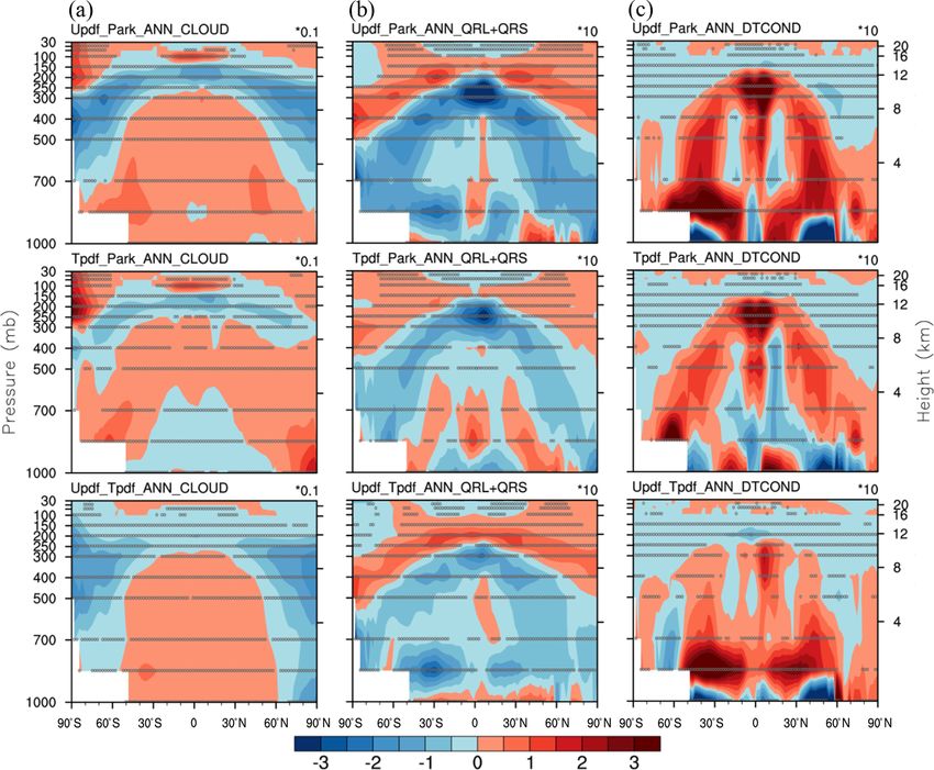
182                                                                             C.-J. Shiu et al.: Macrophysics for climate models

Figure 2. Mean cloud fraction in July (a) from the ERA-Interim reanalysis dataset and (b, c, d) diagnosed from cloud fraction schemes,
with temperature, moisture, and condensates from the ERA-Interim reanalysis provided. From left to right, these schemes are the (b) U_pdf,
(c) T_pdf, and (d) Park macrophysics schemes. Cloud distributions from 100 to 900 hPa are plotted from top to bottom. Also shown are
values of global annual means.

Geosci. Model Dev., 14, 177–204, 2021                                                     https://doi.org/10.5194/gmd-14-177-2021
C.-J. Shiu et al.: Macrophysics for climate models 183
4 Single-column results lated with changes in RH of the GCM grids when compared
to that of the default cloud macrophysics scheme. In fact,
This section presents the analysis of single-column simula- such high correlations between CF and RH seen in the GTS
tions using the TWP-ICE field campaign. We focused on the and Park schemes are not consistent with those of observa-
CF fields and humidity fields to see how the RHc assump- tions as shown in Fig. 3a, suggesting that, in nature, CF and
tion affects these features through humidity partitioning. Five RH are likely to be non-linear.
sets of model experiments were conducted. In addition to the Admittedly, it is not easy to directly use the observational
T_pdf and U_pdf of the GTS and Park schemes, we also CF of the TWP-ICE field campaign to evaluate the per-
include the T_pdf and U_pdf of the GTS scheme with the formance of stratiform cloud macrophysics schemes in the
Slingo ice CF parameterization. These experiments can help SCAM simulations due to the coexistence of other CF types
us to interpret the impacts of RHc on liquid and ice CFs sep- determined by the deep and shallow convective schemes as
arately. well as cloud overlapping treatments in both horizontal and
Figure 3 shows the correlation between CF and RH for vertical directions. As expected, correlation coefficients be-
the three time periods during the TWP-ICE. As expected, tween the simulated and observed CFs are not high and their
the correlation coefficients are quite similar for the individ- values do not differ a lot among the five cloud macrophysics
ual schemes during the active monsoon period when con- schemes (Table S1 in the Supplement).
vective clouds dominated (R = 0.73, Park, vs. 0.71, T_pdf, To minimize possible interference from deep and shal-
vs. 0.70, U_pdf). In contrast, the correlation coefficient be- low convective CFs, we picked up the stratiform-cloud-
tween CF and RH differs during the suppressed monsoon dominated levels and time period to examine the CF–RH
period when stratiform clouds dominated (R = 0.47, Park, distributions. Figure 4 shows scatter plots of RH and CF be-
vs. 0.71, T_pdf, vs. 0.76, U_pdf). The correlation coeffi- tween 50 and 300 hPa determined from observations (Xie et
cient between CF and RH is approximately 20 % higher for al., 2010) and simulated by models run for the suppressed
the stratiform-cloud-dominated period when using T_pdf or monsoon period from the TWP-ICE case. It turns out that the
U_pdf in the GTS scheme. It is also worth mentioning that, CF–RH distributions simulated by the GTS schemes (Fig. 4c
during the monsoon break period when both convective and and f) are closer to those of the observational results (Fig. 4a)
stratiform clouds coexist, the usage of the GTS scheme can except under more overcast conditions (i.e., RH > 70 % and
also increase the correlation between CF and RH by 10 % RH > 110 %). In contrast, the CF–RH distributions simu-
compared to the default Park scheme. Notably, the higher lated by the Park scheme are much less consistent with those
correlation coefficient for stratiform-cloud-dominated areas of observations (Fig. 4d vs. 4a). On the other hand, by ex-
only suggests that the GTS scheme can somehow better sim- cluding PDF-based treatment for the ice cloud fraction in the
ulate the variation of CF associated with RH, for which strat- GTS scheme, a more obvious spread in the CF–RH distribu-
iform cloud macrophysics parameterization normally takes tion is produced (comparing Fig. 4b and c or 4e and f). In
effect in CAM5.3. other words, the comparisons shown in Fig. 4 suggest that
Comparisons between T_pdf with the Slingo ice CF and applying a PDF-based treatment for both liquid and ice CF
the Park scheme can be used to examine the role of apply- parameterizations can simulate the CF–RH distributions in
ing a PDF-based approach in simulating the liquid CF in the better agreement with the observational results.
GTS scheme. The use of a PDF-based approach for calcu-
lating the liquid CF can increase the correlation between CF
and RH by approximately 12 % during the suppressed mon- 5 Global-domain results
soon period (R = 0.69, T_pdf with Slingo, vs. 0.47, Park).
Such an outcome also suggests that implementing a PDF- 5.1 Impacts on cloud fields
based approach for liquid clouds can lead to more reasonable
fluctuations between CF and RH in GCM grids. 5.1.1 Cloud fraction
It turns out that using the PDF-based approach for ice
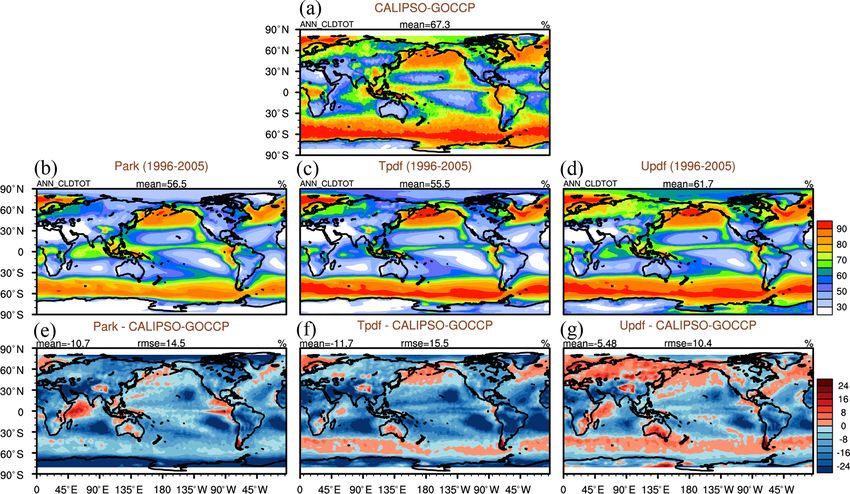
clouds slightly contributes to the increased correlation be- In Fig. 5, total CF simulated by the GTS schemes and the
tween CF and RH, as shown in Fig. 3 with the T_pdf scheme CESM default cloud macrophysics scheme, obtained from
(R = 0.69, T_pdf with Slingo, vs. 0.71, T_pdf) or U_pdf the COSP satellite simulator of the AMWG package of
scheme (R = 0.73, U_pdf with Slingo, vs. 0.76, U_pdf). NCAR CESM, is compared with the total CF in CALIPSO-
Such results also suggest that extending this PDF-based ap- GOCCP. Notably, the following comparisons for the CF and
proach for ice clouds can better simulate changes in the ice associated variables are not only affected by the changes
cloud fraction using an RH-based approach rather than an in the cloud macrophysics but also contributed by the deep
RHc -based approach. Notably, such pair comparisons (i.e., and shallow convective schemes as well as cloud overlap-
T_pdf with Slingo ice cloud fraction scheme vs. T_pdf and ping assumptions in the horizontal and vertical directions.
vs. Park) only reveal the important features of the GTS Both global mean and RMSE values are improved by ap-
scheme, such as how variations in liquid CF are better corre- plying U_pdf in the GTS scheme. The CF simulation result-
https://doi.org/10.5194/gmd-14-177-2021 Geosci. Model Dev., 14, 177–204, 2021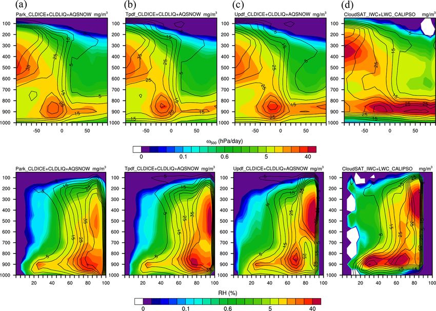
184                                                                                C.-J. Shiu et al.: Macrophysics for climate models

Figure 3. Pressure–time cross-sections of cloud fraction (upper panel) and relative humidity (lower panel) observed by (a) Xie et al. (2010)
and simulated by SCAM with the (b) U_pdf with Slingo ice CF scheme, (c) U_pdf, (d) Park of CAM5.3, (e) T_pdf with Slingo ice CF
scheme, and (f) T_pdf cloud macrophysics schemes. Values shown in the upper sections of panels (a)–(f) represent pressure–time pattern
correlation coefficients between cloud fraction and relative humidity during the whole time period. Similarly, values shown in the lower
sections of panels (a)–(f) represent pattern correlation coefficients between cloud fraction and relative humidity during the first, second, and
third time periods as separated by the dashed lines.

Geosci. Model Dev., 14, 177–204, 2021                                                         https://doi.org/10.5194/gmd-14-177-2021
C.-J. Shiu et al.: Macrophysics for climate models                                                                                                185

Figure 4. Scatter plots of high-level (50–300 hPa) relative humidities and cloud fractions during the suppressed monsoon period of the TWP-
ICE field campaign (26 January to 3 February 2006) observed by (a) Xie et al. (2010) and simulated by SCAM with the (b) U_pdf with
Slingo ice CF scheme, (c) U_pdf, (d) Park of CAM5.3, (e) T_pdf with Slingo ice CF scheme, and (f) T_pdf cloud macrophysics schemes.
Two dashed blue lines are also shown in the figure to enclose the observational RH–CF distributions.

Table 1. Root-mean-square errors (RMSEs) for comparisons of latitude–height cross-sections of CF among the three macrophysical schemes
(Park: default scheme; T_pdf: triangular PDF in the GTS scheme; U_pdf: uniform PDF in the GTS scheme) and observational data from
CloudSat/CALIPSO (Fig. 6). Comparisons are made of the means for five latitudinal ranges and three periods (JJA: June, July, August; DJF:
December, January, February). The smallest RMSE value of the three schemes in each case is bold.

                   Global                   60◦ N–60◦ S                 30◦ N–30◦ S                  30◦ N–90◦ N                  30◦ S–90◦ S
           Park    T_pdf    U_pdf    Park     T_pdf   U_pdf      Park     T_pdf   U_pdf      Park      T_pdf    U_pdf      Park    T_pdf    U_pdf
 Annual    7.15     8.27     6.75    5.25      4.53       4.85   5.84      5.37       5.05    8.78      10.40       8.52   6.46      8.29        6.18
 JJA       7.40    11.30     9.50    6.27      5.64       5.61   6.03      5.96       5.56    8.91      10.60       9.13   6.93     15.50       12.70
 DJF       9.04     9.37     6.99    5.62      5.24       5.38   6.29      5.53       5.36   12.80      13.00      10.00   6.33      7.85        3.82

ing from the use of U_pdf in the GTS scheme is qualita-                    simulation using U_pdf and T_pdf in the GTS scheme agrees
tively similar to that of CloudSat/CALIPSO, especially over                better with that of CloudSat/CALIPSO than that produced by
the mid- and high-latitude regions and for the annual and                  Park under most scenarios (globally, within 60◦ N–60◦ S, and
December–January–February (DJF) simulations (Fig. 6). On                   within 30◦ N–30◦ S), especially for the annual and DJF sim-
the other hand, the results of the Park scheme show clouds                 ulations (Table 1). In contrast, some scenarios show lower
at higher altitudes in the tropics in closer agreement with                RMSEs when the Park scheme is used, e.g., for the June–
CloudSat/CALIPSO than those of U_pdf or T_pdf. Cross-                      July–August (JJA) season globally, within 30–90◦ N, and
section comparison of the zonal height shows that the CF                   within 30–90◦ S. Interestingly, when high latitudes are in-

https://doi.org/10.5194/gmd-14-177-2021                                                              Geosci. Model Dev., 14, 177–204, 2021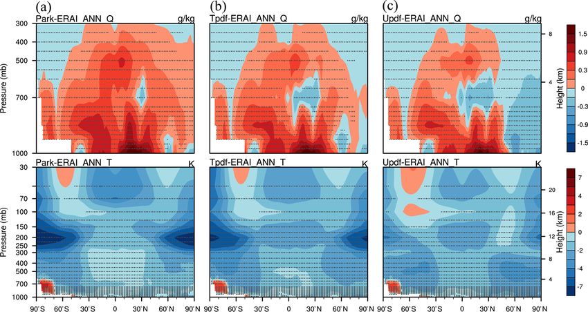
186                                                                          C.-J. Shiu et al.: Macrophysics for climate models

Figure 5. Total CF from (a) CALIPSO-GOCCP and simulated by the three schemes: (b) the default Park, (c) T_pdf, and (d) U_pdf, using
the COSP satellite simulator of the NCAR CESM model. Differences between the simulated and observed total CFs derived from (e) the
default Park, (f) T_pdf, and (g) U_pdf schemes. Also shown are values of global annual means (mean) and root mean square error (rmse)
evaluated against CALIPSO-GOCCP.

cluded (i.e., 30–90◦ N and 30–90◦ S), U_pdf still results in         for the three schemes and CloudSat/CALIPSO for the an-
the smallest RMSE values, except for during the JJA season.          nual, JJA, and DJF means. For the annual mean, U_pdf re-
It is evident that some CFs are existing at the upper level in       sults in the smallest RMSE at all levels except at 125 mbar,
the Antarctic in JJA when U_pdf or T_pdf of GTS is used.             for which the Park scheme yields the smallest RMSE (Ta-
However, such high CFs are not seen in CloudSat/CALIPSO              ble 2). For JJA, the Park scheme is closer to the observations
observations, suggesting that the usage of GTS schemes               aloft (100–200 mbar) and nearest the surface (900 mbar). For
could cause significant biases in CFs under such environmen-         DJF, U_pdf again performs best at most levels except 100 and
tal conditions. This is of course highly related to the ice CF       125 mbar, for which T_pdf is slightly better, while for JJA,
schemes of GTS. More observation-constrained adjustments             U_pdf is only best for most of the levels below 300 mbar.
or tuning of the ice CF schemes of GTS are needed to reduce          Overall, U_pdf in the GTS scheme results in better latitude–
the biases in CFs in similar atmospheric environments like           longitude CF distributions for 300–900 mbar for the annual,
the upper level of the Antarctic winter. Potential tuning pa-        DJF, and JJA means, suggesting improvements in CF simu-
rameters of ice CF scheme of GTS are sup and RHc which               lation for middle and low clouds.
are discussed in Sect. 5.6.3.                                           When annual, DJF, and JJA mean vertical CF profiles are
   We also compared the annual latitude–longitude distribu-          averaged over the entire globe and between 30◦ N and 30◦ S,
tions of CF at different specific pressure levels (Fig. 7). The      U_pdf in the GTS scheme can produce a global simula-
use of U_pdf resulted in a CF simulation relatively simi-            tion close to that of CloudSat/CALIPSO for 200–850 mbar
lar to that of CloudSat/CALIPSO for mid-level clouds, i.e.,          (Fig. S1 in the Supplement). In contrast, there is a large dis-
300–700 mbar, particularly for the mid- and high latitudes.          crepancy between the simulated and observed CFs over the
However, none of the CF parameterizations are able to sim-           tropics. Although the GTS schemes can simulate CF profiles
ulate stratocumulus clouds effectively, as revealed at the 850       above 100 mbar, the height of the maximum CF is lower than
and 900 mbar levels. For high clouds, the GTS and Park               that of CloudSat/CALIPSO. In contrast, the height of the
schemes exhibit observable differences regarding the maxi-           maximum CF simulated by the Park scheme is similar to that
mum CF level. Table 2 summarizes the RMSE values for the             of CloudSat/CALIPSO but overestimated in CF. As before,
latitude–longitude distribution of CFs at nine specific levels       when compared with CloudSat/CALIPSO, U_pdf in the GTS

Geosci. Model Dev., 14, 177–204, 2021                                                  https://doi.org/10.5194/gmd-14-177-2021
C.-J. Shiu et al.: Macrophysics for climate models                                                                                187

Table 2. RMSEs for comparisons between CF at nine pressure levels, as simulated by the three macrophysical schemes (Park, T_pdf,
U_pdf) and observational data from CloudSat/CALIPSO (Fig. 7). The comparisons are made for three periods (JJA: June, July, August; DJF:
December, January, February). The smallest RMSE value of the three schemes in each case is bold.

                                            Annual                      JJA                        DJF
                                    Park    T_pdf    U_pdf      Park   T_pdf     U_pdf    Park    T_pdf   U_pdf
                      100 mbar      6.07     5.40      4.71     4.85   12.70      10.10    7.88    3.94     4.20
                      125 mbar      4.70     5.56      4.80     6.13   12.60      10.10    5.96    4.56     4.81
                      200 mbar      7.23     8.34      6.78     9.80   14.90      11.90    8.64    6.57     6.46
                      300 mbar     10.80     9.63      7.98    11.60   12.90      10.80   12.40   11.70     9.06
                      400 mbar     11.80    10.50      6.93    12.40   10.50       9.55   12.70   13.90     8.06
                      500 mbar     11.00    11.50      7.65    11.90   10.60       9.28   11.70   13.40     8.50
                      700 mbar      8.64     9.47      8.19     9.63   10.80       9.46   10.70   11.10     9.41
                      850 mbar     14.30    14.20     12.00    14.80   15.40      12.80   16.10   15.30    13.20
                      900 mbar     12.50    15.10     12.30    13.30   16.60      13.60   15.10   16.40    12.90

scheme results in the smallest RMSE and the largest correla-           are plotted against ω500, although for CWC plotted against
tion coefficient of the three schemes, whether or not the lower        RH300–1000, the Park scheme yields the smallest RMSE
levels are included except in JJA at 125 mbar, for which Park          (Table 3). Overall, these comparisons yield results that are
yields the smallest RMSE (Table S2). The reason for exclud-            consistent with the general characteristics of most CMIP5
ing the lower levels from the statistical results is that there        models, as found by Su et al. (2013). GCMs in general sim-
may be a bias for low clouds retrieved by CloudSat due to              ulate the distribution of cloud fields better with respect to a
radar-signal blocking by deep convective clouds.                       dynamical parameter as opposed to a thermodynamic param-
   The different degrees of changes for the global and trop-           eter.
ical CFs can be attributed to the relative roles of cumulus               It is also worth noting that the use of U_pdf yields a 20 %–
parameterizations (both deep and shallow) and stratus cloud            30 % improvement in R when plotted against RH300–1000
macrophysics and/or microphysics for the different latitudi-           for the two latitudinal ranges, 30◦ N–30◦ S and 60◦ N–60◦ S.
nal regions. It is expected that the GTS scheme can alter CF           The observable improvement in a thermodynamic parame-
simulations in the mid- and high-latitude areas more than in           ter is an indication of the uniqueness of this GTS scheme, in
the tropics because more stratiform clouds occur in those ar-          that it is capable of simulating the variation in cloud fields
eas. It is also interesting to note that, although it is known that    relative to that in RH fields. There are also slight improve-
more convective clouds exist in the tropics (i.e., the cumulus         ments in cloud fields with respect to large-scale dynamical
parameterization contributes more to the grid CF), the GTS             parameters. On the other hand, the Park scheme results in an
scheme can also affect the CF simulation over the tropics to           approximately 20 % improvement in R when plotted against
some extent.                                                           RH300–1000 for the global domain, suggesting that the de-
                                                                       fault Park scheme still simulates cloud fields better over the
5.1.2   Cloud fraction and cloud water content                         high latitudinal regions. It is thus worth addressing the like-
                                                                       lihood that the different CF and CWC results for the differ-
In Figs. 8 and 9, the distributions of CWC and CF as func-             ent latitudinal ranges simulated using the GTS scheme in-
tions of large-scale vertical velocity at 500 mbar (ω500) or           duce cloud–radiation interaction distinct from that simulated
mean RH averaged between 300 and 1000 mbar (RH300–                     in the Park scheme. Such changes in cloud–radiation inter-
1000) are evaluated against CloudSat/CALIPSO observa-                  action would modify not only the thermodynamic fields but
tions for 30◦ N–30◦ S and 60◦ N–60◦ S. Figures 8 and 9 show            also the dynamic fields in the GCMs. These changes are in
that the model simulations are all qualitatively more sim-             turn likely to affect the climate mean state and variability.
ilar to each other than to the observations. Further statis-           We assess and compare these potential effects in the follow-
tical comparisons are shown in Table 3. It is encouraging              ing subsection.
to note that, in addition to the slight improvements in CF
for both of these latitudinal ranges, the use of U_pdf in              5.2     Effects on annual mean climatology
the GTS scheme results in a CWC simulation that is more
consistent with CloudSat/CALIPSO, whether it is plotted                GTS schemes tend to produce smaller RMSE values for most
against ω500 or RH300–1000. The RMSE and correlation                   of the global mean values of the radiation flux, cloud radia-
coefficient (R) values in Table 3 confirm this. For global             tive forcing, and CF parameters shown in Table 4, suggesting
simulations, using U_pdf also results in better agreement              that the GTS scheme is capable of simulating the variability
with CloudSat/CALIPSO for both CF and CWC when they                    of these variables. Furthermore, the assumed U_pdf shape

https://doi.org/10.5194/gmd-14-177-2021                                                     Geosci. Model Dev., 14, 177–204, 2021
188 C.-J. Shiu et al.: Macrophysics for climate models
Table 3. RMSE and R values for comparisons between CF and CWC simulated by the three macrophysical schemes (Park, T_pdf, and
U_pdf) and plotted against vertical velocity at 500 mbar (ω500) or averaged RH for 300–1000 mbar (RH300–1000, obtained from the ERA-
Interim reanalysis) and observational data from CloudSat/CALIPSO (Figs. 9 and 10). The comparisons are made for three latitudinal ranges.
The smallest RMSE or largest R value of the three schemes in each case is bold.
RMSE Global 60◦ N–60◦ S 30◦ N–30◦ S
Park T_pdf U_pdf Park T_pdf U_pdf Park T_pdf U_pdf
CWC 11.10 10.90 9.83 11.40 11.20 10.10 14.10 13.80 12.50
OMEGA at 500 mbar
CF 7.65 7.26 6.13 7.55 7.23 6.24 8.13 8.07 7.21
CWC 8.73 9.69 11.60 13.50 15.10 11.80 19.10 18.00 12.00
RH at 300–1000 mbar
CF 17.90 18.30 13.90 15.40 17.30 12.70 18.80 18.30 12.90
R Global 60◦ N–60◦ S 30◦ N–30◦ S
Park T_pdf U_pdf Park T_pdf U_pdf Park T_pdf U_pdf
CWC 0.73 0.77 0.80 0.74 0.77 0.80 0.60 0.66 0.74
OMEGA at 500 mbar
CF 0.84 0.85 0.89 0.85 0.85 0.88 0.83 0.82 0.84
CWC 0.64 0.54 0.45 0.44 0.34 0.62 0.22 0.25 0.55
RH at 300–1000 mbar
CF 0.31 0.40 0.59 0.51 0.46 0.68 0.45 0.45 0.66
Table 4. Global annual means (mean) and RMSE values for comparisons with the observed values (obs) for a selection of climatic parameters
simulated by the three cloud macrophysical schemes (Park, T_pdf, and U_pdf). The smallest RMSE value or closest global mean of the three
schemes in each case is bold.
Parameter Obs Mean RMSE
Park T_pdf U_pdf Park T_pdf U_pdf
RESTOA_CERES-EBAF 0.81 4.18 3.25 − 1.06 12.39 10.43 11.11
FLUT_CERES-EBAF 239.67 234.97 237.88 238.14 8.78 6.73 6.50
FLUTC_CERES-EBAF 265.73 259.06 259.65 260.45 7.55 7.12 6.48
FSNTOA_CERES-EBAF 240.48 239.15 241.14 237.08 13.97 11.64 12.79
FSNTOAC_CERES-EBAF 287.62 291.26 291.31 291.70 7.08 7.09 7.58
LWCF_CERES-EBAF 26.06 24.10 21.77 22.31 6.78 6.77 6.21
SWCF_CERES-EBAF −47.15 −52.11 − 50.18 −54.61 15.98 12.90 15.43
PRECT_GPCP 2.67 2.97 3.04 3.14 1.09 1.10 1.15
PREH20_ERAI 24.25 25.64 24.90 24.45 2.56 2.05 2.03
CLDTOT_CloudSat + CALIPSO 66.82 64.11 70.77 70.09 9.87 11.38 9.76
CLDHGH_CloudSat + CALIPSO 40.33 38.17 44.79 40.22 9.37 9.28 8.17
CLDMED_CloudSat + CALIPSO 32.16 27.22 30.41 31.26 8.03 6.95 6.28
CLDLOW_CloudSat + CALIPSO 43.01 43.63 43.67 46.19 12.78 18.06 16.17
CLDTOT_CALIPSO-GOCCP 67.25 56.43 55.45 61.72 14.38 15.37 10.28
CLDHGH_CALIPSO-GOCCP 32.04 25.57 22.48 24.46 9.04 11.30 10.16
CLDMED_CALIPSO-GOCCP 18.09 11.21 14.55 18.19 8.35 6.34 6.02
CLDLOW_CALIPSO-GOCCP 37.95 33.24 33.16 38.41 10.63 11.33 9.98
TGCLDLWP (ocean) 79.87 42.55 40.68 48.74 40.92 42.37 35.16
U_200_MERRA 15.45 16.18 15.87 15.66 2.52 2.11 1.94
T_200_ERAI 218.82 215.58 215.76 216.84 4.03 3.37 2.13
Geosci. Model Dev., 14, 177–204, 2021 https://doi.org/10.5194/gmd-14-177-2021C.-J. Shiu et al.: Macrophysics for climate models 189
appears to perform better for outgoing longwave radiation
flux, longwave cloud forcing (LWCF), and CF at various lev-
els, whereas the T_pdf assumption is better for simulating net
and shortwave radiation flux at the top of the atmosphere as
well as shortwave cloud forcing (SWCF) (Table 4). On the
other hand, the Park scheme is better for simulating clear-
sky net shortwave radiation flux and precipitation. Smaller
RMSE values can also be seen for parameters such as to-
tal precipitable water, total-column cloud liquid water, zonal
wind at 200 mbar (hereafter, U_200), and air temperature at
200 mbar (hereafter, T_200) when U_pdf of GTS is used. For
global annual means, U_pdf simulates net radiation flux at
the top of the atmosphere, all- and clear-sky outgoing long-
wave radiation flux, and precipitable water as well as U_200
and T_200 in closer agreement with observations. In con-
trast, the Park scheme is better for simulating global mean
variables such as net shortwave radiation flux at the top of
the atmosphere, longwave cloud forcing, and precipitation.
T_pdf simulates SWCF closest to the observational mean.
Overall, the averaged RMSE values of the 10 parame-
ters are 0.97 and 0.96 for U_pdf and T_pdf, respectively, in
the GTS schemes (Fig. 10), suggesting that using the GTS
schemes would result in global simulation performance more
or less similar to that of the Park scheme. It is also worth
noting that the biases in RH are smallest when U_pdf in the
GTS scheme is used (Table S3 in the Supplement). In con-
trast, T_pdf results in the smallest biases for SWCF, sea level
pressure, and ocean rainfall within 30◦ N–30◦ S. On the other
hand, the Park scheme produces the smallest biases regard-
ing mean fields such as LWCF, land rainfall within 30◦ N–
30◦ S, Pacific surface stress within 5◦ N–5◦ S, zonal wind at
300 mbar, and temperature.
Comparisons of latitude–height cross-sections of RH and
ERA-Interim show that the GTS schemes tend to simulate
RH values smaller than the default scheme does, especially
for high-latitude regions (> 60◦ N and 60◦ S), as shown in
Fig. 11. In general, in terms of RH, using T_pdf in the GTS
scheme results in better agreement with ERA-Interim (Ta-
ble S4). Figure 12 shows that the Park and T_pdf schemes
are wetter than ERA-Interim almost everywhere and that the
uniform scheme is sometimes drier. Table S5a further sug-
gests that specific humidity simulated by the GTS schemes
is slightly more consistent with ERA-Interim than the Park
scheme. Comparisons of air temperature show that the three
schemes tend to have cold biases almost everywhere. How-
ever, it is interesting to note that the cold biases are reduced
to some extent when using the GTS schemes compared to the
default scheme, as is evident in the smaller values of RMSE
shown in Table S5b. These effects on moisture and temper-
ature are likely to result in changes in the annual cycle and
seasonality of climatic parameters. Such observable changes
Figure 6. Latitude–height cross-sections of (a) annual, (b) June–
in RH, clouds (both CF and CWC), and cloud forcing suggest
July–August (JJA), and (c) December–January–February (DJF)
mean CFs from CloudSat/CALIPSO data (upper left) and the Park that the GTS scheme will simulate cloud macrophysics pro-
(upper right), U_pdf (lower left), and T_pdf (lower right) schemes. cesses in GCMs quite differently from the Park scheme, due
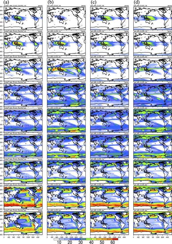
https://doi.org/10.5194/gmd-14-177-2021 Geosci. Model Dev., 14, 177–204, 2021190 C.-J. Shiu et al.: Macrophysics for climate models Figure 7. CFs at nine pressure levels (one pressure level per row; top to bottom: 100, 125, 200, 300, 400, 500, 700, 850, and 900 mbar) from (a) CloudSat/CALIPSO observational data and simulated by (b) the default Park, (c) U_pdf, and (d) T_pdf schemes. Geosci. Model Dev., 14, 177–204, 2021 https://doi.org/10.5194/gmd-14-177-2021
C.-J. Shiu et al.: Macrophysics for climate models                                                                                 191

Figure 8. Vertical distribution of CF (contour lines) and CWC (colors) as functions of two large-scale parameters: vertical velocity at
500 mbar (ω500, upper four panels) and relative humidity averaged between 300 and 1000 mbar (RH300–1000, lower four panels) for the
latitudinal range 30◦ N–30◦ S. Columns present simulations by the (a) Park, (b) T_pdf, and (c) U_pdf schemes, and (d) observational data
from CloudSat/CALIPSO.

to the use of a variable-width PDF that is determined based           GTS schemes is closer to that of ERA-Interim than that simu-
on grid-mean information.                                             lated by the Park scheme (Table S6). Furthermore, the U_pdf
                                                                      assumption results in a better annual U_200 cycle than the
5.3   Changes in the annual cycle of climatic variables               T_pdf assumption, especially for 60◦ N–60◦ S. This further
                                                                      supports the argument that this GTS scheme can effectively
Figure 13 shows the annual cycle of precipitable water sim-           modulate global simulations, with respect to both thermody-
ulated by the three schemes. The magnitude of precipitable            namic and dynamical climatic variables.
water simulated by the GTS schemes is closer to the ERA-                 Figure 15 displays the global mean annual cycles of sev-
Interim data than the Park simulation is (Table S6). Interest-        eral parameters simulated by the three schemes and the cor-
ingly, U_pdf results in slightly better agreement with ERA-           responding parameters from observational data. The GTS
Interim than T_pdf for the region 60◦ N–60◦ S. This implies           scheme simulations of total precipitable water (TMQ) are
that the GTS scheme would alter the moisture field for both           close to that of ERA-Interim; indeed, U_pdf almost exactly
RH and precipitable water in GCMs. These results are rela-            reproduces the ERA-Interim TMQ. However, we must ad-
tively more realistic with respect to both the moisture field         mit that such good agreement of the global mean is partly
and CF and CWC (Figs. 8 and 9), and are likely to yield a             due to offsetting wet and dry differences from ERA-Interim.
more reasonable cloud–radiation interaction in the GCMs. It           The GTS schemes also produce a more reasonable global
is therefore also worth examining any differences in dynamic          mean annual cycle for outgoing longwave radiation (FLUT).
fields, for example, in the annual U_200 cycle, between the           It is probably due to the reduced CF simulated by the GTS
three schemes and the ERA-Interim data (Fig. 14). Like the            scheme compared to the Park scheme even though the cloud
annual cycle of precipitable water, U_200 simulated by the

https://doi.org/10.5194/gmd-14-177-2021                                                     Geosci. Model Dev., 14, 177–204, 2021
192 C.-J. Shiu et al.: Macrophysics for climate models
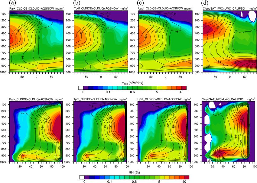
Figure 9. Vertical distribution of CF (contour lines) and CWC (colors) as functions of two large-scale parameters: ω500 (upper four panels)
and RH300–1000 (lower four panels) for the latitudinal range 60◦ N–60◦ S. Columns present simulations by the (a) Park, (b) T_pdf, and
(c) U_pdf, and (d) observational data from CloudSat/CALIPSO.
top heights simulated by GTS are lower than observations in each pair-wise combination of the three schemes. Qualita-
the tropics. Interestingly, for SWCF, T_pdf yields a simula- tively consistent changes in CF are apparent for the GTS
tion closer to the observations than the other two schemes, schemes, e.g., an increase in the highest clouds over the trop-
which is consistent with the features of the global annual ics and a decrease below them, a decrease in 150–400 mbar
mean of SWCF shown in Fig. 10 and Table S3. However, clouds over the midlatitudes, a decrease in 300–700 mbar
for LWCF, the annual cycle simulated by Park is closest to clouds over the high latitudes, an increase in 300–700 mbar
the observations. The U_pdf of the GTS scheme also results clouds over the tropics to midlatitudes, and an increase in low
in improvements in U_200 and T_200 (Fig. 15). The RMSEs clouds over the high-latitude regions. The GTS schemes also
for all of these comparisons confirm these results (Table S7). yield a significant increase in CF at atmospheric levels higher
than 300 mbar over the high-latitude regions (Fig. 16). These
5.4 Changes in cloud–radiation interaction changes affect the radiation calculations to some extent. In
addition, CWC is also affected by the GTS schemes (Figs. 8
As mentioned in Sect. 5.1, usage of the GTS cloud macro- and 9). The combined effects of the changes in CF and CWC
physics schemes would affect the cloud fields, i.e., CF and are likely to result in changes in cloud–radiation interaction.
CWC. This, in turn, is likely to affect global simulations with In addition, although there are significant changes in CF at
respect to both mean climatology and the annual cycles of high atmospheric levels in the high-latitude regions, the com-
many climatic parameters (as discussed in Sect. 5.2 and 5.3) bined effect of CF and CWC on QRL + QRS is quite small,
through cloud–radiation interaction. Figure 16 compares CF, due to the low CWC values over this region. The changes
radiation heating rate (i.e., longwave heating rate plus short- in moisture processes, i.e., DTCOND (Fig. 16), also sug-
wave heating rate, hereafter QRL + QRS), and temperature gest that the combined effects of the changes in the thermo-
tendencies due to moist processes (hereafter, DTCOND) for
Geosci. Model Dev., 14, 177–204, 2021 https://doi.org/10.5194/gmd-14-177-2021You can also read