Modelling the future evolution of glaciers in the European Alps under the EURO-CORDEX RCM ensemble - The Cryosphere
←
→
Page content transcription
If your browser does not render page correctly, please read the page content below
The Cryosphere, 13, 1125–1146, 2019
https://doi.org/10.5194/tc-13-1125-2019
© Author(s) 2019. This work is distributed under
the Creative Commons Attribution 4.0 License.

Modelling the future evolution of glaciers in the European Alps
under the EURO-CORDEX RCM ensemble
Harry Zekollari1,2,a , Matthias Huss1,3 , and Daniel Farinotti1,2
1 Laboratory of Hydraulics, Hydrology and Glaciology (VAW), ETH Zürich, Zurich, Switzerland
2 Swiss Federal Institute for Forest, Snow and Landscape Research (WSL), Birmensdorf, Switzerland
3 Department of Geosciences, University of Fribourg, Fribourg, Switzerland
a now at: Department of Geoscience and Remote Sensing, Delft University of Technology, Delft, the Netherlands

Correspondence: Harry Zekollari (zharry@ethz.ch)

Received: 1 December 2018 – Discussion started: 19 December 2018
Revised: 1 March 2019 – Accepted: 27 March 2019 – Published: 9 April 2019

Abstract. Glaciers in the European Alps play an important           ited warming, the inclusion of ice dynamics reduces the pro-
role in the hydrological cycle, act as a source for hydroelec-      jected mass loss and that this effect increases with the glacier
tricity and have a large touristic importance. The future evo-      elevation range, implying that the inclusion of ice dynamics
lution of these glaciers is driven by surface mass balance and      is likely to be important for global glacier evolution projec-
ice flow processes, of which the latter is to date not included     tions.
explicitly in regional glacier projections for the Alps. Here,
we model the future evolution of glaciers in the European
Alps with GloGEMflow, an extended version of the Global
Glacier Evolution Model (GloGEM), in which both sur-                1   Introduction
face mass balance and ice flow are explicitly accounted for.
The mass balance model is calibrated with glacier-specific          In the coming century, glaciers are projected to lose a sub-
geodetic mass balances and forced with high-resolution re-          stantial part of their volume, maintaining their position as
gional climate model (RCM) simulations from the EURO-               one of the main contributors to sea-level rise (Slangen et al.,
CORDEX ensemble. The evolution of the total glacier vol-            2017; Bamber et al., 2018; Marzeion et al., 2018; Moon et al.,
ume in the coming decades is relatively similar under the           2018; Parkes and Marzeion, 2018). In the European Alps the
various representative concentrations pathways (RCP2.6, 4.5         retreat of glaciers will have a large impact, as glaciers play
and 8.5), with volume losses of about 47 %–52 % in 2050             an important role in river runoff (e.g. Hanzer et al., 2018;
with respect to 2017. We find that under RCP2.6, the ice            Huss and Hock, 2018; Brunner et al., 2019), hydroelectricity
loss in the second part of the 21st century is relatively lim-      production (e.g. Milner et al., 2017; Patro et al., 2018) and
ited and that about one-third (36.8 % ± 11.1 %, multi-model         touristic purposes (e.g. Fischer et al., 2011; Welling et al.,
mean ±1σ ) of the present-day (2017) ice volume will still          2015; Stewart et al., 2016).
be present in 2100. Under a strong warming (RCP8.5) the                In order to understand how the ca. 3500 glaciers of the
future evolution of the glaciers is dictated by a substantial in-   European Alps (Pfeffer et al., 2014) (Fig. 1a) will react to
crease in surface melt, and glaciers are projected to largely       changing 21st century climatic conditions (e.g. Gobiet et al.,
disappear by 2100 (94.4 ± 4.4 % volume loss vs. 2017). For          2014; Christidis et al., 2015; Frei et al., 2018; Stoffel and
a given RCP, differences in future changes are mainly de-           Corona, 2018), to date, models of various complexity have
termined by the driving global climate model (GCM), rather          been used. Regional glacier evolution studies in the Alps
than by the RCM, and these differences are larger than those        (Zemp et al., 2006; Huss, 2012; Salzmann et al., 2012; Lins-
arising from various model parameters (e.g. flow parameters         bauer et al., 2013) have focused on methods in which ice dy-
and cross-section parameterisation). We find that under a lim-      namics are not explicitly accounted for, and the glacier evo-
                                                                    lution is based on parameterisations. One of the first studies

Published by Copernicus Publications on behalf of the European Geosciences Union.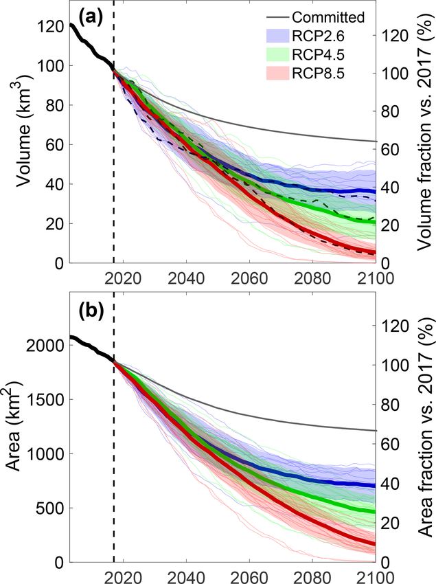
1126                                   H. Zekollari et al.: Modelling the future evolution of glaciers in the European Alps

to estimate the future evolution of all glaciers in the Euro-     1985–2015 climate. This model was recently also used by
pean Alps was performed by Haeberli and Hoelzle (1995),           Goosse et al. (2018) to simulate the transient evolution of
who used glacier inventory data and combined this with a pa-      71 Alpine glaciers over the past millennium.
rameterisation scheme to predict the future evolution of the         Here, we explore the potential of using a coupled SMB–
Alpine ice mass. In another study, Zemp et al. (2006) utilised    ice flow model for regional projections, by modelling the fu-
a statistical calibrated equilibrium-line altitude (ELA) model    ture evolution of glaciers in the European Alps with such
to estimate future area losses. More recently, Huss (2012)        a model. For this, we extend the Global Glacier Evolu-
modelled the future evolution of about 50 large glaciers          tion Model (GloGEM) of Huss and Hock (2015) by intro-
with a retreat parameterisation and extrapolated these find-      ducing an ice flow component. We refer to this model as
ings to the entire European Alps. The future evolution of         GloGEMflow in the following. Our approach is furthermore
glaciers in the European Alps was also modelled as a part of      novel, as glacier-specific geodetic mass balance estimates are
global studies, relying on methods that parameterise glacier      used for model calibration, and the future glacier evolution
changes through volume–area–length scaling (Marzeion et           relies directly on regional climate change projections from
al., 2012; Radić et al., 2014) and methods in which geom-        the EURO-CORDEX (COordinated Regional climate Down-
etry changes are imposed based on observed changes (Huss          scaling EXperiment applied over Europe) ensemble (Jacob
and Hock, 2015). These regional and global studies generally      et al., 2014; Kotlarski et al., 2014). This is, to the best of
suggest a glacier volume loss of about 65 %–80 % between          our knowledge, the first regional glacier modelling study in
the early 21st century and 2100 under a moderate warming          the Alps directly making use of this high-resolution regional
(RCP2.6 and RCP4.5) and an almost complete disappearance          climate model (RCM) output. In contrast to a forcing with a
of glaciers under warmer conditions (RCP8.5).                     general circulation model (GCM), an RCM driven by a GCM
   For certain well-studied Alpine glaciers, 3-D high-            can provide information on much smaller scales, support-
resolution ice flow models have been used to simulate their       ing a more in-depth impact assessment and providing pro-
future evolution (e.g. Le Meur and Vincent, 2003; Le Meur         jections with much detail and more accurate representation
et al., 2004, 2007; Jouvet et al., 2009, 2011; Zekollari et       of localised events.
al., 2014). These studies are of large interest to better un-        Through novel approaches in terms of (i) climate forcing,
derstand the glacier dynamics and the driving mechanisms          (ii) inclusion of ice dynamics, (iii) the use of glacier-specific
behind their future evolution, but individual glacier charac-     geodetic mass balance estimates for model calibration and by
teristics hamper extrapolations of these findings to the re-      (iv) relying on a vast and diverse dataset on ground-truth data
gional scale (Beniston et al., 2018). Given the computational     for model calibration and validation, we aim at improving
expenses related to running such complex models, and due          future glacier change projections in the European Alps. As
to the lack of field measurements needed for model calibra-       part of our analysis, we explore how the new methods and
tion and validation (e.g. mass balance, ice thickness and sur-    data utilised could affect other regional and global glacier
face velocity measurements), these models cannot be applied       evolution studies.
for every individual glacier in the European Alps. A possi-
ble alternative consists of using a regional glaciation model
(RGM), in which a surface mass balance (SMB) component            2     Data
and an ice dynamics component are coupled and applied
                                                                  2.1    Glacier geometry
over an entire mountain range, i.e. not for every glacier in-
dividually (Clarke et al., 2015). However, running a RGM          For every individual glacier in the European Alps, the
at a high spatial resolution remains computationally expen-       outlines are taken from the Randolph Glacier Inven-
sive, and the discrepancy between the model complexity and        tory (RGI v6.0) (RGI Consortium, 2017) (Fig. 1). These
the uncertainty in the various boundary conditions persists.      glacier outlines are mostly from an inventory derived by Paul
In an RGM study for western Canada, Clarke et al. (2015)          et al. (2011) using Landsat Thematic Mapper scenes from
showed that relative area and volume changes are well rep-        August and September 2003 (for 96.7 % of all glaciers in-
resented by such a model but that large, local present-day        cluded in the RGI). The surface hypsometry is derived from
differences between observed and modelled glacier geome-          the Shuttle Radar Topography Mission (SRTM) version 4
tries can exist after a transient simulation. To date, the most   (Jarvis et al., 2008) digital elevation model (DEM) from 2000
adequate and sophisticated method to model the evolution of       (RGI Consortium, 2017).
all glaciers in the European Alps thus consists of modelling         The ice thicknesses of the individual glaciers is calculated
every glacier individually with a coupled ice flow–surface        according to the method of Huss and Farinotti (2012) in 10 m
mass balance model. A pilot study in this direction was un-       elevation bands, which relies on ice volume flux estimates.
dertaken by Maussion et al. (2019), with the newly released       The horizontal distance (1x) between the elevation bands is
Open Global Glacier Model (OGGM), in which steady-state           determined from the elevation difference (1y) and the band-
simulations are performed for every glacier worldwide based       average local surface slope (s):
on standard (i.e. non-calibrated) model parameters under the

The Cryosphere, 13, 1125–1146, 2019                                                   www.the-cryosphere.net/13/1125/2019/
H. Zekollari et al.: Modelling the future evolution of glaciers in the European Alps                                                     1127

Figure 1. Distribution of glaciers (red areas) in the European Alps. Outlines correspond to the glacier geometries at the Randolph Glacier
Inventory (RGI v6.0) date (typically 2003) (Paul et al., 2011; RGI Consortium, 2017). The hill shade in the background is from the Shuttle
Radar Topography (SRTM) DEM (Jarvis et al., 2008). Glaciers discussed in this paper and the Supplement are highlighted in yellow: (I) Mer
de Glace and Argentière, (II) Grosser Aletsch, Unteraar and Rhone, (III) Morteratsch, (IV) Careser, (V) Hintereisferner, Kesselwandferner,
Taschachferner, Gepatschferner and Langtaler Ferner. The inset shows the cumulative glacier area and volume, sorted by decreasing glacier
length. The dotted line is the division between glaciers longer (left) and shorter (right) than 1 km. Glacier area is from the Randolph Glacier
Inventory (RGI v6.0) (RGI Consortium, 2017); volume and length are as derived from an updated version of Huss and Farinotti (2012).

                                                                          of 45◦ is taken for α, the effect of which is assessed in the
      1y                                                                  uncertainty analysis (Sect. 6.3).
1x =       .                                                     (1)
     tan s
To determine the band-average slope s, all values below the               2.2   Climate data
5 % quantile are discarded, as well as all values above a
threshold (typically around the 80 % to 90 % quantile) deter-             The 2 m air temperature and precipitation are used to repre-
mined based on the skewness of the slope distribution func-               sent the climatic conditions at the glacier surface for SMB
tion. Subsequently, the glacier geometry is interpolated to a             calculations (Sect. 3.1). For the past (1951–2017), we rely
regular, horizontal grid along-flow. Through this approach,               on the ENSEMBLES daily gridded observational dataset (E-
possible glacier branches and tributaries are not explicitly ac-          OBS v.17.0) on a 0.22◦ grid (Haylock et al., 2008). This
counted for, avoiding complications and potential problems                E-OBS product represents past events closely (for example,
related to solving the little-known mass transfer in these con-           the heat wave of the summer of 2003; Fig. 2b), allowing for
nections. As such, this approach is less sensitive to uncertain-          detailed comparisons between observed and modelled sur-
ties in glacier outlines and topography compared to meth-                 face mass balances (Sect. 4.1). We prefer using an observa-
ods in which glacier branches are explicitly accounted for                tional dataset compared to a reanalysis product (e.g. ERA-
(e.g. Maussion et al., 2019) but may in some cases oversim-               INTERIM, as used in Huss and Hock, 2015), as the for-
plify the mass flow for complex glacier geometries (e.g. with             mer has a higher resolution and goes further back in time.
several branches). Glacier cross sections are represented as              Additionally, relying on higher-resolution RCM simulations
symmetrical trapezoids. The bedrock elevation is determined               forced with reanalysis data is not possible, as for several fu-
in order to ensure local volume and area conservation. These              ture simulations (see next section), a related simulation is not
symmetrical trapezoids deviate from a rectangular cross sec-              available. This would furthermore complicate the model val-
tion by an angle α (see Fig. S1 in the Supplement). A value               idation for the past, as the past climatic conditions would be

www.the-cryosphere.net/13/1125/2019/                                                             The Cryosphere, 13, 1125–1146, 2019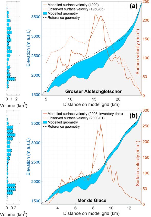
1128                                   H. Zekollari et al.: Modelling the future evolution of glaciers in the European Alps

different for every model RCM simulation, while the obser-        relevant at the annual scale. Furthermore, variability in pre-
vational data provide a single past temperature and precipi-      cipitation does not have a direct effect on the calibrated SMB
tation forcing.                                                   parameters (as is the case for temperatures via the degree-day
   For the future, we use climate change projections from the     factors; see Sect. 3.1.).
EURO-CORDEX ensemble (Jacob et al., 2014; Kotlarski et
al., 2014), from which all available simulations at 0.11◦ reso-   2.3    Mass balance
lution (ca. 12 km horizontal resolution) are considered. This
corresponds to a total of 51 simulations, consisting of differ-   The SMB model component is calibrated (Sect. 3.1) with
ent combinations of nine RCMs, six GCMs and various real-         glacier-specific geodetic mass balances taken from the World
isations (r1i1p1, r12i1p1, r2i1p1, r3i1p1), forced with three     Glacier Monitoring Service (WMGS) database (WGMS,
representative concentration pathways (RCPs; Fig. 2 and Ta-       2018). Most of these geodetic mass balances were derived
ble S1 in the Supplement) (van Vuuren et al., 2011; IPCC,         by Fischer (2011) (Austria), Berthier et al. (2014) (France,
2013). The three considered RCPs are (i) a peak-and-decline       Italy and Switzerland) and M. Fischer et al. (2015) (Switzer-
scenario with a rapid stabilisation of atmospheric CO2 lev-       land). About 1500 glaciers (ca. 38 % by number) have a
els (RCP2.6), (ii) a medium mitigation scenario (RCP4.5)          glacier-specific geodetic mass balance observation. Since
and (iii) a high-emission scenario (RCP8.5). Note that while      larger glaciers are overrepresented in this sample, however,
country-specific projections such as the ones recently re-        this corresponds to about 60 % of the total Alpine glacier
leased with CH2018 report for Switzerland (CH2018, 2018)          area. For glaciers for which several geodetic SMB obser-
exist, which rely on simulations from the EURO-CORDEX             vations are available, the one closest to the reference pe-
ensemble, these cannot be applied in a uniform way over the       riod 1981–2010 is selected for model calibration. In the case
entire Alps.                                                      no geodetic mass balance observation for the specific glacier
   For modelling the future SMB, debiased RCM trends from         is available, an observation from a nearby glacier is chosen.
the EURO-CORDEX ensemble are imposed on the E-OBS                 The respective observation is selected based on (i) the hor-
grid based on the nearest grid cell. To ensure a consistency      izontal distance (in km) and (ii) the relative difference in
between the observational (E-OBS, used for past) and RCM          area (unitless). We multiply these two values and consider
(EURO-CORDEX, used for future) climatic data, a debias-           the minimum as the most suitable glacier to supply a mass
ing procedure is applied (Huss and Hock, 2015). Here, addi-       balance observation for the unmeasured glacier. The replace-
tive (temperature) and multiplicative (precipitation) monthly     ment thus represents a nearby glacier that is relatively similar
biases are calculated to ensure a consistency in the magni-       in size. The effect of this approach is evaluated in Sect. 4.1.
tude of the signal over the common time period. These bi-            For model validation (Sect. 4.1), we rely on in situ
ases are assumed to be constant in time and are superimposed      SMB observations provided by the WGMS Fluctuations
on the RCM series. Furthermore, RCM temperature series            of Glaciers Database (WGMS, 2018), consisting of 1672
are adjusted to account for differences in year-to-year vari-     glacier-wide annual balances and 12 097 annual balances for
ability between the observational and the RCM time series.        specific glacier elevation bands. Note that we prefer using
Accounting for the differences in interannual variability is      geodetic mass balance over SMB observations for calibra-
crucial to ensure the validity of the calibrated model param-     tion, as we argue that it is more important to have a good
eters for the future RCM projections (Hock, 2003; Farinotti,      coverage for model calibration than for its validation. Fur-
2013). For each month m, the standard deviation of tempera-       thermore, geodetic mass balances are becoming increasingly
tures over the common time period is calculated for both the      available at the regional scale (e.g. Brun et al., 2017; Braun
observational (σobs,m ) and the RCM data (σRCM,m ). For each      et al., 2019) and outgrow the availability of in situ measure-
month m and year y of the projection period, the interannual      ments, making the adopted strategy applicable to other re-
variability of the RCM air temperatures Tm,y is corrected as      gions.

Tm,y,corrected = Tm,25 + Tm,y − Tm,25 φm .                 (2)
                                                                  3     Methods
Here Tm,25 is the average temperature in a 25-year period         GloGEMflow consists of a surface mass balance component
centred around y, and φm corresponds to σobs,m /σRCM,m .          (Sect. 3.1), which is taken from GloGEM (Huss and Hock,
This correction is applied over the period 1970–2017, which       2015), and an ice flow component (Sect. 3.2). These two
is the overlap period for which all RCM simulations and E-        components are combined to calculate the temporal evolu-
OBS data are available. This procedure ensures consistency        tion of the glacier (Sect. 3.3).
in interannual variability while allowing for future changes
in the temperature variability given by the RCMs (Fig. 2).        3.1    Surface mass balance modelling
For precipitation, which enters the SMB calculations as a cu-
mulative quantity, no correction for interannual variability is   Here, we briefly describe the SMB model component, with
applied, as the monthly differences in variability are not that   an emphasis on the settings specific to this study. For a more

The Cryosphere, 13, 1125–1146, 2019                                                   www.the-cryosphere.net/13/1125/2019/
H. Zekollari et al.: Modelling the future evolution of glaciers in the European Alps                                                  1129

Figure 2. Debiased temperature anomaly (a: annual b: June–July–August) and debiased precipitation anomaly (c: annual and d: October–
March) between 1950 and 2100 relative to 1961–1990 (horizontal dotted line). All values correspond to the mean over all grid cells used
in this study, weighed by the glacier area (at inventory date) in every cell. The thick black line represents the evolution of the variables
for observational period (E-OBS dataset). The coloured thin lines represent the evolution for individual RCM simulations from the EURO-
CORDEX ensemble (51 in total; see Table S1), and the thick lines are the RCM simulation means (one per RCP).

elaborate description, we refer to the description in Huss and          relying on monthly temperature lapse rates derived from the
Hock (2015).                                                            RCMs. Subsequently, model calibration parameters (degree-
   For every glacier, the model is forced with monthly tem-             day factors, precipitation scaling factor) are adapted as a
perature and precipitation series (Sect. 2.2) from the E-OBS            part of a glacier-specific three-step calibration procedure that
(past) or RCM (future) grid cell closest to the glacier’s cen-          aims at reproducing the observed geodetic mass balance. In
tre point. Accumulation is computed from precipitation, and             the first step, overall precipitation is multiplied by a scaling
a threshold is used to differentiate between liquid and solid           factor varying between 0.8 and 2.0. This initial step focuses
precipitation. This threshold is defined as an interval from            on the precipitation, as this is the variable that is expected
0.5 to 2.5 ◦ C, within which the snow / rain ratio is linearly in-      to be the most poorly reproduced due to resolution issues,
terpolated. The melt is calculated for every grid cell from a           spatial variability and local effects (e.g. snow redistribution)
classic temperature-index melt model (Hock, 2003), in which             (e.g. Jarosch et al., 2012; Hannesdóttir et al., 2015; Huss and
a distinction between snow, firn and ice melt is made based             Hock, 2015). If this step does not allow the observed geodetic
on different degree-day factors. Refreezing of rain and melt            SMB to be reproduced within a 10 % bound, in a second step
water is also accounted for and calculated from snow and                the degree-day factors for snow and ice are modified. Here,
firn temperatures based on heat conduction (see Huss and                the degree-day factor of snow is allowed to vary between
Hock, 2015). Huss and Hock (2015) showed that the added                 1.75 and 4.5 mm d−1 K−1 (default value is 3 mm d−1 K−1 ;
value of using a simplified energy balance model (Oerle-                see Hock, 2003), and the degree-day factor of ice is adjusted
mans, 2001) was limited and that it did not perform bet-                to ensure a 2 : 1 ratio between both degree-day factors. In an
ter than the temperature-index melt model when validated                eventual third and final step, the air temperature is modified
against SMB measurements.                                               through a systematic shift over the entire glacier (see Fig. 2a
   For every individual glacier the climatic data are scaled            in Huss and Hock, 2015, for more details).
from the gridded product to the individual glacier at a rate
of 2.5 % per 100 m elevation change for precipitation and by

www.the-cryosphere.net/13/1125/2019/                                                           The Cryosphere, 13, 1125–1146, 2019
1130                                     H. Zekollari et al.: Modelling the future evolution of glaciers in the European Alps

3.2    Ice flow modelling

The ice flow is modelled explicitly with a flowline model
for all glaciers longer than 1 km at the RGI inventory date.
These 795 glaciers represent ca. 95 % of the total volume
and 86% of the total area of all glaciers in the European Alps
(Fig. 1, inset). For glaciers shorter than 1 km, mass transfer
within the glacier is limited, and the time evolution is mod-
elled through the 1h parameterisation (Huss et al., 2010b), in
line with the original GloGEM setup (Huss and Hock, 2015).
   The dynamics of the ice flow component are solved
through the Shallow-Ice Approximation (SIA) (Hutter,
1983), in which basal shear (τ ) is proportional to the local
                                            ∂s
ice thickness (H ) and the surface slope ( ∂x  ):

            ∂s
τ = −ρgH       ,                                             (3)
            ∂x
where g = 9.81 m s−2 is gravitational acceleration, while the
ice density ρ is set to 900 kg m−3 . In our model, mass trans-
port is expressed through a Glen (1955) type of flow law, in
which the depth-averaged velocity u (m a−1 ) is defined as          Figure 3. Model initialisation for creating a glacier with the refer-
                                                                    ence length and volume at the inventory date.
       2A n
u=        τ H.                                               (4)
      n+2
                                                                    where D is the diffusivity factor (m2 a−1 ):
Here n = 3 is Glen’s flow law exponent, and A is the                                      −1
deformation-sliding factor (Pa−3 a−1 ) that accounts for the                  2              ∂s
                                                                    D=A           τ nH 2             .                               (7)
effects of the ice rheology on its deformation, sliding and var-            n+2              ∂x
ious others effects (e.g. lateral drag). Basal sliding is implic-   The continuity equation is solved using a semi-implicit
itly accounted for through this approach and not treated sep-       forward scheme by relying on an intermediate time step
arately from internal deformation, given the relatively large       (i.e. sub-time-step update) in which the geometry is updated.
uncertainties associated with it. Basal sliding and internal de-       The initialisation consists of closely reproducing the
formation are both linked to the surface slope and the local        glacier geometry at the inventory date. At first, constant cli-
ice thickness and have been shown to have similar spatial           matic conditions are imposed, until a steady state is obtained,
patterns on Alpine glaciers (e.g. Zekollari et al., 2013), jus-     which represents the glacier in 1990 (Fig. 3). These con-
tifying an approach in which both are combined (e.g. Gud-           stant climate conditions correspond to the mean SMB un-
mundsson, 1999; Clarke et al., 2015).                               der the 1961–1990 climate, to which a SMB perturbation is
                                                                    applied (detailed below). Subsequently, the glacier is forced
3.3    Time evolution and initialisation                            with E-OBS data and evolves transiently from 1990 until the
                                                                    glacier-specific inventory date (typically 2003). We opt for
The glacier geometry is updated at every time step through
                                                                    a 1990 steady-state glacier, as the glaciers in the European
the continuity equation:
                                                                    Alps were generally not too far off equilibrium around this
∂H                                                                  period, with SMBs for many glaciers being close to zero
    = ∇ · f + b,                                             (5)    (Huss et al., 2010a; WGMS, 2018). By imposing a steady
 ∂t
                                                                    state in 1990, the glacier length at the inventory date can be
where b is the surface mass balance (m w.e. a−1 ), and ∇ ·f is      influenced. Methodologically, choosing an initial steady state
                                            ∂s
the local divergence of the ice flux (f = D ∂x ). For a transect    before 1990 would be problematic, as in this case the glacier
with a trapezoidal shape, with a basal width wb and a surface       geometry would not determine the glacier length at the in-
width ws (Fig. S1), this becomes (see Oerlemans, 1997)              ventory date anymore, as the period between the steady state
              "                                                    and the inventory date exceeds the typical Alpine glacier re-
                                   ∂h

∂H         1     wb + ws ∂ D ∂x                                     sponse time of several years to a few decades (e.g. Oerle-
     =−
 ∂t       ws         2          ∂x                                  mans, 2007; Zekollari and Huybrechts, 2015).
               wb +ws  #                                            The glacier volume and length at the inventory date are
            ∂h ∂       2                                            matched by calibrating two variables (Fig. 3). The first cal-
     + D                      + b,                           (6)
            ∂x       ∂x                                             ibration variable is the deformation-sliding factor A, which

The Cryosphere, 13, 1125–1146, 2019                                                       www.the-cryosphere.net/13/1125/2019/
H. Zekollari et al.: Modelling the future evolution of glaciers in the European Alps                                                   1131

Figure 4. Evaluation of modelled SMB against observations from the WGMS (2018) database. All observations are included, except those
that do temporally overlap with the geodetic mass balance observations (used for calibration). Scatterplots (a, c) and frequency of mis-
fits (b, d) of modelled vs. measured glacier-wide annual balances (a, b) and annual mass balances per elevation band (c, d). Dashed red lines
in (b) and (d) represent the zero misfit. In (a) and (c), n corresponds to the number of observations, RMSE is the root-mean-square error,
MAD is the median absolute deviation and r 2 is the coefficient of determination.

mainly determines the volume of the glacier at the inventory             geodetic mass balance observations. As the aim is to evaluate
date. The reason for this resides in the role that A has on the          the performance of the SMB model (rather than the coupled
local ice flux, which in turn affects the local ice thickness and        SMB–ice flow model) and to incorporate as many valida-
thus the ice volume; see Eqs. (4)–(7). The second calibration            tion points as possible (which is only possible after 1990 for
variable is an SMB offset in the 1961–1990 climatic con-                 the dynamic simulations), these calculations are based on the
ditions used to construct a 1990 steady-state glacier, which             glacier geometry at the inventory date. The observed glacier-
mainly determines the length of the steady-state glacier (as             wide annual mass balances are in general well reproduced,
the geometry is such that the integrated SMB equals zero).               with a root-mean-square error (RMSE) of 0.74 m w.e. a−1 , a
Note that a change in steady-state length causes the glacier             median absolute deviation (MAD) of 0.67 m w.e. a−1 and a
length to change at the inventory date as well. An opti-                 systematic error (mean misfit) of −0.09 m w.e. a−1 (Fig. 4a
misation procedure is used, in which at each iteration the               and b). Furthermore, the good agreement between observed
deformation-sliding factor and the SMB offset are informed               and modelled balances for glacier elevation bands (r 2 =
from previous iterations (see Appendix A for details). This              0.60; Fig. 4b and d) suggests that, despite not being cal-
results in a fast convergence to the desired state, i.e. a glacier       ibrated to this, the modelled and observed SMB gradient
with the same length and volume as the reference geome-                  are in reasonably good agreement. When only considering
try (from Huss and Farinotti, 2012) at the inventory date. It            SMB measurements on glaciers that have no observed geode-
should be noticed that the reference volume is itself a model            tic mass balance (i.e. glaciers for which the geodetic mass
result (Huss and Farinotti, 2012) and thus also holds uncer-             balance used to calibrate the model was extrapolated from
tainties. The choice for the 1990 steady state and the effect            other, nearby glaciers), the misfit between modelled and ob-
this has on the calibration procedure are assessed in the un-            served values increases only little (RMSE = 0.79 m w.e. a−1 ;
certainty analysis (Sect. 6.3).                                          MAD = 0.72 m w.e. a−1 ; mean misfit = −0.19 w.e. a−1 ), in-
                                                                         dicating that the method used to extrapolate the geodetic
                                                                         mass balances to unmeasured glaciers performs well. Finally,
4     Model validation                                                   sensitivity tests were performed with the SMB model being
                                                                         forced with historical RCM output (instead of E-OBS). The
4.1    Surface mass balance                                              tests indicate that the RCMs, despite not being forced with
                                                                         reanalysis data, are producing general SMB tendencies that
The modelled SMB is evaluated by using independent, ob-                  are relatively close to those obtained when forcing the model
served glacier-wide annual balances and annual balances for              with E-OBS data (similar mean values; see Fig. S2; similar
glacier elevation bands (Fig. 4). In order to ensure that the            interannual variability: σSMB,EOBS = 0.66 m w.e. a−1 ; mean
validation procedure is independent from the calibration, val-           σSMB,RCM = 0.58 m w.e. a−1 ).
idation is only performed with observations that do not tem-
porally overlap with the geodetic mass balances used for
calibration (see Sects. 2.3 and 3.1) and for glaciers without

www.the-cryosphere.net/13/1125/2019/                                                            The Cryosphere, 13, 1125–1146, 2019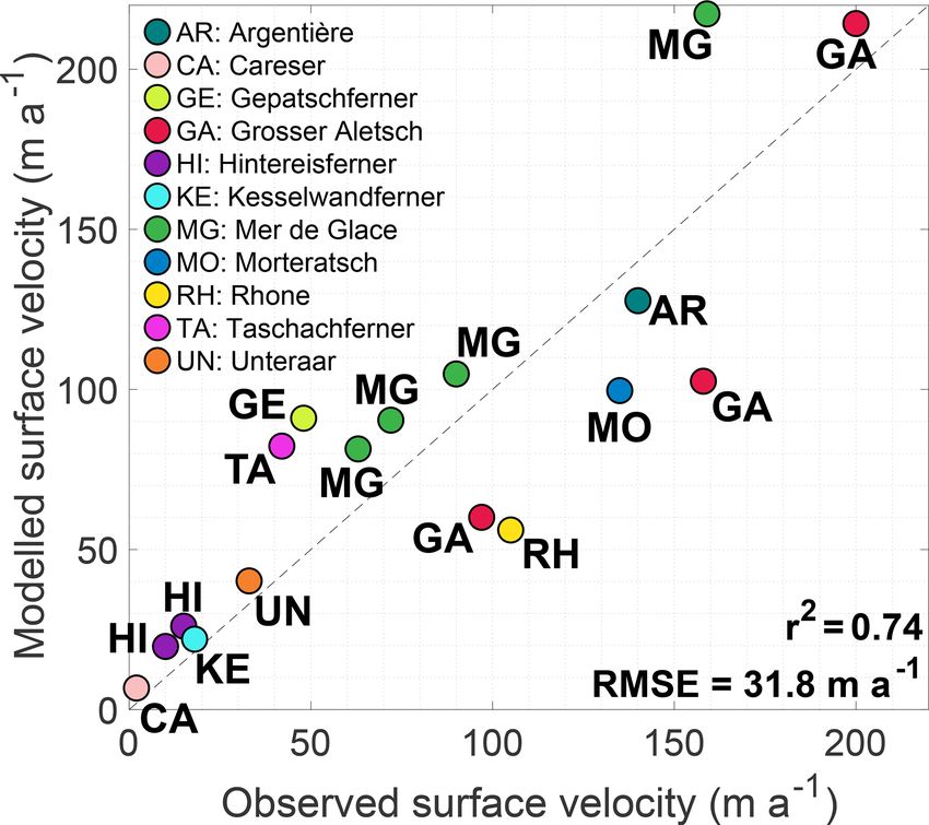
1132                                    H. Zekollari et al.: Modelling the future evolution of glaciers in the European Alps

4.2    Glacier geometry

The glaciers are calibrated to match the length and volume
at inventory date within 1 % (σ between reference and mod-
elled volume or length of 0.6 % or 0.5 % of the reference
value, respectively). Despite not being calibrated to it, the
observed glacier area is also closely reproduced (σ of 0.7 %).
In the calibration procedure the distribution of ice with eleva-
tion is unconstrained, but nonetheless the reference volume–
elevation distribution of various glaciers, based on Huss and
Farinotti (2012), updated to RGI v6.0, is well reproduced.
We use two well-studied glaciers to illustrate this (Fig. 5),
namely the Grosser Aletschgletscher (Valais, Switzerland)
and the Mer de Glace (Mont-Blanc massif, France). Also for
the other 793 glaciers longer than 1 km, a good match is ob-
tained (see Supplement).

4.3    Glacier dynamics

In our approach the mass transport between grid cells is lin-
early dependent on the deformation-sliding factor A, which
is thus important for ice dynamics. The calibrated values
of A for every individual glacier do not have a distinct
spatial pattern, nor do they correlate with glacier length or
glacier elevation (Fig. S3). It is not straightforward to com-
pare the values of the deformation-sliding factor to other
values from literature used to describe ice deformation and
mass transport (such as rate factors), as different formula-
tions and approaches are utilised, e.g. the inclusion/exclusion
of a shape factor, explicit/implicit treatment of basal slid-      Figure 5. Comparison between reference and modelled (i) glacier
ing and different geometry representations. However, it ap-        geometry, (ii) volume–elevation distribution and (iii) surface veloc-
pears that the spread in the modelled deformation-sliding          ities for Grosser Aletschgletscher (a) and Mer de Glace (b). Refer-
factors, which results from the fact that this value repre-        ence geometries and volume–elevation distribution are at inventory
sents several physical processes and uncertainties in our ap-      date (2003) and based on Huss and Farinotti (2012). Observed sur-
proach, largely falls within the literature range values of        face velocities for Grosser Aletschgletscher are from Zoller (2010)
rate/creep factors (Fig. S3). Furthermore, the calibrated me-      and correspond to 1950/1985 point averages, while observed ve-
dian (1.1×10⁻¹⁶ Pa−3 a−1 ) and mean (1.3×10⁻¹⁶ Pa−3 a−1 )          locities for the Mer de Glace are derived from 2000/2001 SPOT
values are relatively close to the widely used rate/creep factor   imagery (Berthier and Vincent, 2012).
from Cuffey and Paterson (2010) based on several modelling
studies (0.8 × 10⁻¹⁶ Pa−3 a−1 ).
   In the lower parts, where many glaciers have a distinct         for Grosser Aletschgletscher and the Mer de Glace (Fig. 5).
tongue, a comparison between observed and modelled sur-            Some discrepancies are likely linked to the simplicity of our
face velocities is possible (surface velocities correspond to      model and uncertainties in various boundary conditions, but
1.25 times the depth-integrated velocities, since we treat         they may in part also be related to the different time periods
basal sliding implicitly; see, e.g. Cuffey and Paterson, 2010,     between the observations and the modelled state.
p. 310). This is more complicated for the higher parts of
the glaciers, where glaciers may be broad and have various         4.4   Past glacier evolution
branches, which we do not explicitly account for in our ap-
proach. In general, our model is able to reproduce the ob-         Modelled past glacier length and area changes are compared
served surface velocities for the lower glacier parts despite      to observations for the time period between the inventory
its simplicity. Based on a set of surface velocity observations    date (typically 2003) and present day (2017). Periods be-
from the literature (see Fig. 6 and Table S2), a large range       fore 2003 are not considered, as the effect from the im-
of surface velocities, from 1 to > 200 m a−1 , is well repro-      posed 1990 steady state may still be pronounced on the ini-
duced (r 2 = 0.76; RMSE = 31.8 m a−1 ), without a tendency         tial glacier evolution (1990–2003). Furthermore, before the
for consistent under- or overestimation. This is illustrated       inventory date, length and area changes from the 1h parame-

The Cryosphere, 13, 1125–1146, 2019                                                      www.the-cryosphere.net/13/1125/2019/

H. Zekollari et al.: Modelling the future evolution of glaciers in the European Alps                                              1133

                                                                       8 km the root-mean-square error (RMSE) between the ob-
                                                                       served and modelled 2003–2017 retreat is only 155 m, corre-
                                                                       sponding to approx. 30 % of the mean observed (490 m) and
                                                                       modelled (540 m) retreat over this time period.

                                                                       4.4.2   Glacier area

                                                                       Glacier area changes in the European Alps have been de-
                                                                       rived in various studies. Depending on the time period
                                                                       considered and the ensemble of glaciers studied, estimated
                                                                       glacier area changes vary broadly from −1.5 % a−1 to
                                                                       −0.5 % a−1 . Paul et al. (2004) derived area changes for
                                                                       938 Swiss glaciers and used these to extrapolate a loss of
                                                                       675 km2 for all glaciers in the European Alps over the pe-
                                                                       riod 1973–1998/1999 (corresponding to a 22 % mass loss, or
                                                                       about −0.85 % a−1 /26 km2 a−1 ). For Austria, area changes
Figure 6. Observed vs. modelled surface velocities for selected        of −1.2 % a−1 were observed for the period 1998–2004/2012
glaciers in the European Alps. For some glaciers several data points   (A. Fischer et al., 2015). On longer timescales, Fischer et
exist, consisting of different locations on the glacier. More infor-   al. (2014) derived a relative area loss of 0.75 % a−1 for
mation concerning the surface velocities and corresponding refer-
                                                                       the period 1973–2010 over Switzerland, while for the pe-
ences is given in the Supplement (Table S2). For glacier location,
see Fig. 1.
                                                                       riod 2003–2009 an area loss of 1.3 % a−1 was obtained
                                                                       for glaciers in the eastern Swiss Alps. French glaciers
                                                                       lost about one-quarter of their area between 1967/1971
terisation (which we apply for glaciers < 1 km) are not avail-         and 2006/2009, corresponding to a change of −0.7 % a−1
able, as here the starting point is the observed geometry at           (Gardent et al., 2014), while Italian glaciers lost about 30 %
the inventory date. Note that past glacier volume changes are          of their area over the 1959/1962–2005/2011 period (i.e. av-
available (e.g. M. Fischer et al., 2015) but that these are not        erage of −0.6 % a−1 ) (Smiraglia et al., 2015).
used for validation, as they were utilised for calibrating the            Between 2003 and 2017, we model a glacier area loss of
SMB model component.                                                   223 km2 (16 km2 a−1 ), corresponding to a relative area loss
                                                                       of 11.3 % (vs. mean area over this time period), or 0.8 % a−1 .
4.4.1   Glacier length                                                 These numbers are difficult to directly compare with values
                                                                       from the literature, as different time periods are considered
The modelled length changes between the inventory                      (implying also a different reference area), and as the area
date (2003) and 2017 are compared to observations for all              losses strongly depend on size of the considered glaciers
52 Swiss glaciers longer than 3 km that are included in                (e.g. Paul et al., 2004; Fischer et al., 2014), which also varies
the Swiss glacier monitoring network (GLAMOS) (Glacio-                 between studies. However, a qualitative comparison suggests
logical Reports, 1881–2017) (Fig. 7). Note that other                  that the modelled area changes are in general slightly lower
length records are also available for non-Swiss glaciers               than the observations. This discrepancy is mostly related to
(e.g. Leclercq et al., 2014) but that these were not consid-           the fact that many present-day glaciers have frontal regions
ered to ensure a consistency in derived length records. De-            and ablation areas with almost stagnant ice and in some cases
spite the model’s simplicity, the general trends in glacier re-        also consist of disconnected ice patches, which our model is
treat are relatively well reproduced and there is no general           not able to capture with a simple cross-section parameteri-
tendency for over- or underestimation. A few outliers exist            sation. By modifying the cross section through increasing λ,
(highlighted in Fig. 7), of which the underestimations can be          a higher modelled area loss is obtained, in closer agreement
attributed to a detachment of the lower and upper parts of             with observations. However, a higher value of λ may be un-
the glacier, which cannot be captured in our modelling setup.          realistic (i.e. produce an area change close to observations
Overestimated retreat rates (Ferpècle, Montminé and Stein)             for the wrong reasons), and the effect of a different λ value
occur for glaciers where the modelled ice thickness in the             is found to have a very limited effect on the future modelled
frontal region at the inventory date is likely to be lower than        volume and area changes (this is addressed in Sect. 6.3).
the reference state and/or where the ice thickness is underes-
timated in the reference case. When the three glaciers with
underestimations due to a disconnection are omitted, the cor-          5   Future glacier evolution
relation between the observed and modelled glacier retreat is
r 2 = 0.37 (p value < 1×10⁻³ ). For large glaciers, the retreat        Our projections suggest that from 2017 to 2050 a total vol-
is particularly well reproduced: e.g. for glaciers longer than         ume loss of about 50 % and area loss of about 45 % will occur

www.the-cryosphere.net/13/1125/2019/                                                          The Cryosphere, 13, 1125–1146, 2019
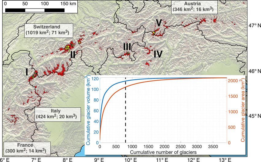
1134                                     H. Zekollari et al.: Modelling the future evolution of glaciers in the European Alps

Figure 7. Observed vs. modelled glacier retreat (length change) between 2003 and 2017 for all 52 glaciers longer than 3 km monitored by
GLAMOS (Glaciological Reports, 1881–2017). Point size is proportional to glacier area (as is the case for the colour bar).

and that this evolution is independent of the RCP (Fig. 8 and         loss (−25 km2 a−1 ) are relatively constant until 2070 (Fig. 8),
Table 1). This evolution is related to the fact that the annual       after which they decrease to ca. −0.5 and −15 km2 a−1 ,
and summer temperature differences between the RCPs in-               respectively. By 2100, the Alps are largely ice-free under
crease with time and are thus relatively limited in the coming        RCP8.5, with volume losses of −94.4±4.4 % and area losses
decades (see Fig. 2a and b). Furthermore, a part of the future        of −91.1 ± 5.4 % with respect to 2017 (see Table 1).
evolution is committed, i.e. being a reaction to the present-            An analysis in which the relative volume loss is compared
day glacier geometry, which is too large for the present-day          to present-day glacier characteristics (volume, area, length,
climatic conditions for most glaciers in the European Alps            median elevation, mean elevation, minimum elevation, max-
(e.g. Zekollari and Huybrechts, 2015; Gabbud et al., 2016;            imum elevation, centre of mass and elevation range) reveals
Marzeion et al., 2018; see discussion in Sect. 6.1.1).                that under RCP2.6, the relative volume loss has the highest
   By the end of the century the modelled glacier volume              correlation with the glacier elevation range (Fig. 9 and Ta-
and area are largely determined by the RCP that was used              ble S3; r 2 = 0.57). The maximum glacier elevation, which is
to force the climate model (Fig. 8). Under RCP2.6, in 2100            strongly related to the glacier elevation range, also describes
about 65 % of the present-day (2017) volume and area are              the volume changes well (Table S3, r 2 = 0.38). This is also
lost (−63.2 ± 11.1 % and −62.1 ± 8.4 % respectively; multi-           evident from the spatial distribution of the relative volume
model mean ±1σ ; Table 1, Fig. 8a). Most of the ice loss              loss, which shows the losses are the lowest for mountain
occurs in the next three decades, corresponding to about              ranges that reach above 3600–3700 m (from west to east): the
70 %–75 % of the total changes for the period 2017–2100               Écrin massif, the Mont Blanc Massif, the Monte Rosa Mas-
(Table 1), after which the ice loss clearly reduces (Fig. 8).         sif, the Bernese Alps, the Bernina Range, in the Dolomites,
For an intermediate warming scenario (RCP4.5), about three-           in the Ötzal Alps and the High Tauern (Fig. 9a). The ice loss
quarters of the present-day volume (−78.8 ± 8.8 %) and area           is particularly strong below 3200 m a.s.l., where (for a given
(−74.9 ± 8.3 %) are lost by the end of the century (Fig. 8,           elevation band) more than half of the present-day volume
Table 1). In contrast to the glacier evolution under RCP2.6,          disappears by 2100 under RCP2.6 (Fig. 10). The remaining
under RCP4.5 a substantial part of the loss takes place in the        ice at these lower elevations is typically from medium-sized
second part of the 21st century. However, the largest changes         and large glaciers, which maintain a relatively large accumu-
still occur in the coming three decades, with about 60 % of           lation area that supplies mass to the lower glacier regions.
the total changes for the period 2017–2100 (see Table 1). For         This is for instance the case for the Mer de Glace (France)
RCP8.5, the rates of volume loss (−1.5 km3 a−1 ) and area             and Grosser Aletschgletscher (Switzerland), where ice is still

The Cryosphere, 13, 1125–1146, 2019                                                        www.the-cryosphere.net/13/1125/2019/
H. Zekollari et al.: Modelling the future evolution of glaciers in the European Alps                                            1135

Table 1. Overview of multi-model mean future glacier evolution based on RCM simulations from the EURO-CORDEX ensemble. The
evolution under the mean SMB obtained from the 1988–2017 climatic conditions represents the committed loss.

                                               Volume in km3                                  Area in km2
                                       (and relative change vs. 2017)                (and relative change vs. 2017)
                                               2050                 2100                     2050                2100
                                               71.4                60.8                   1277.9             1091.2
                    1988–2017
                                    (−25.9 ± 7.4 %)     (−36.9 ± 6.3 %)           (−23.3 ± 7.7 %)    (−34.5 ± 6.5 %)
                                               51.7                35.9                   1037.6               701.7
                    RCP2.6
                                   (−47.0 ± 10.3 %)    (−63.2 ± 11.1 %)           (−43.9 ± 9.7 %)    (−62.1 ± 8.4 %)
                                               50.0                20.7                   1006.9               464.2
                    RCP4.5
                                    (−48.8 ± 9.2 %)     (−78.8 ± 8.8 %)           (−45.6 ± 8.0 %)    (−74.9 ± 8.3 %)
                                               47.1                 5.4                     948.2              165.4
                    RCP8.5
                                   (−51.8 ± 11.5 %)     (−94.4 ± 4.4 %)           (−48.8 ± 9.2 %)    (−91.1 ± 5.4 %)

present below 2500 m a.s.l. by the end of the century un-               6     Discussion
der most EURO-CORDEX RCP2.6 simulations (Fig. 11a
and b). However, both glaciers lose a considerable part of              6.1     Drivers of future evolution
their length throughout the century, but whereas Grosser
Aletschgletscher (Fig. 11a) will likely still be retreating by          6.1.1    Committed loss
the end of the century, the Mer de Glace will be relatively
stable in 2100 under most EURO-CORDEX simulations                       Part of the future mass loss is committed and related to the
and under certain simulations even experience readvance                 present-day glacier distribution of ice. Many glaciers have
episodes after 2080 (Fig. 11b). Glaciers that spread over a             a present-day mass excess at low elevation, where locally
higher elevation range are likely to suffer even fewer changes          the flux divergence cannot compensate for the very negative
and in some cases only lose their low-lying tongues (Fig. 9b).          SMB, resulting in a negative thickness change (see Eq. 5 )
In contrast, glaciers at low elevation mostly disappear by the          (e.g. Johannesson et al., 1989; Adhikari et al., 2011; Zekol-
end of the century, even under the moderate RCP2.6 scenario.            lari and Huybrechts, 2015; Marzeion et al., 2018). To assess
This is illustrated for Langtaler Ferner (Austria), which is sit-       the importance of this committed effect, we investigate the
uated below 3300 m a.s.l. and is projected to (almost) entirely         glacier evolution under present-day climatic conditions. For
disappear somewhere between 2050 and 2100 depending on                  this, the model is constantly forced with the mean 1988–
the specific RCM simulation (Fig. 11c).                                 2017 SMB (Fig. 8). Under these conditions, the committed
   The glacier elevation range is also the variable with the            loss is particularly strong for small glaciers at lower eleva-
highest correlation with respect to the future relative volume          tions (e.g. Langtaler Ferner, with a committed volume loss
changes under RCP4.5 (r 2 = 0.63) and RCP8.5 (r 2 = 0.51)               of ca. 90 % by 2100), while for larger glaciers this effect is
(Table S3). Under these RCPs, except for the related max-               more limited. Overall, the Alpine glaciers are projected to
imum elevation, also the present-day glacier length corre-              lose about 35 % of their present-day volume and area by the
lates significantly (p < 10−3 ) with the 2017–2100 volume               end of the century. Simulations with other recent reference
loss (r 2 = 0.23 and r 2 = 0.20 respectively). This indicates           periods (e.g. 2008–2017) resulted in similar committed ice
that under more extreme scenarios the ice loss is very pro-             losses. This suggests that under RCP2.6, about 60 % of the
nounced at all elevations (see also Fig. 11d and e), and the            ice losses for the period 2017–2100 are committed losses,
remaining ice in 2100 is mainly a relict of the present-day             while the remaining 40 % are related to additional warming.
ice distribution; i.e. ice at the end of the century is only re-           The committed losses are in agreement with simulations
maining where there is much ice at present at relatively high           performed by Maussion et al. (2019). In steady-state exper-
elevation.                                                              iments with the Open Global Glacier Model in which all
                                                                        glaciers, starting from their geometry at the inventory date
                                                                        (typically 2003), are subjected to the 1985–2015 randomised
                                                                        climate, Maussion et al. (2019) project ice volume losses of
                                                                        around 55 % over a 100-year time period for the European
                                                                        Alps. In our simulations, over the period 2000–2100, about
                                                                        50 % of the ice mass is lost for an experiment in which the
                                                                        model is forced with the E-OBS product until 2017 and sub-

www.the-cryosphere.net/13/1125/2019/                                                           The Cryosphere, 13, 1125–1146, 2019
1136 H. Zekollari et al.: Modelling the future evolution of glaciers in the European Alps
glacier characteristics reveals that the effect of including ice
dynamics is particularly linked to the glacier elevation range
(r 2 = 0.27; p < 10−3 ) and to a lesser extent to other (related)
glacier characteristics, such as glacier length (r 2 = 0.08),
mean slope (r 2 = 0.04), minimum elevation (r 2 = 0.07) and
the maximum elevation (r 2 = 0.20) (all values based on
multi-model mean for RCP2.6). Under RCP2.6, glaciers with
a large elevation range (typically > 1000 m) experience less
loss in the dynamic model on average compared to when be-
ing forced with the 1h parameterisation (Fig. 12). The mech-
anism behind this is the following:
i. At the inventory date, the glacier geometry is very sim-
ilar in both approaches, as the dynamically modelled
glacier is as close as possible to the observed geome-
try (see Sect. 4.2), which is the starting point for the 1h
parameterisation.
ii. Initially, the total glacier volume evolution is largely
similar in both approaches, as the glaciers are subject to
the same climatic conditions, and their geometry does
barely differ.
iii. However, for glaciers with a large elevation range, rela-
tively more ice is removed at middle and high elevations
in the 1h parameterisation, while in the dynamic model
the ice loss at the lowest glacier elevations is more pro-
nounced.
Figure 8. Ensemble (a) volume and (b) area evolution for vari- iv. As a consequence, the geometry starts evolving differ-
ous EURO-CORDEX RCM simulations and committed loss (mean
ently between both approaches, and the larger ice mass
1988–2017 conditions). Thin lines are individual RCM simulations
at lower elevation in the 1h parameterisation (and lower
(51 in total, see Table S1). The thick line is the RCP mean and the
transparent bands correspond to one standard deviation. In (a), the ice mass at high elevation) translates into a more nega-
coloured dotted lines correspond to the model simulations that are tive specific glacier mass balance for the 1h parame-
closest to the multi-model mean. The vertical dotted line represents terisation (vs. the dynamic model), resulting in a higher
the year 2017 and marks the transition between E-OBS and EURO- mass loss.
CORDEX forcing.
v. In the second half of the 21st century, most glaciers
stabilise under a limited to moderate warming (their
glacier-wide mass balance evolves towards zero). Given
sequently with a constant 1988–2017 mean SMB (grey line
the lower mass and area at middle to high elevations
in Fig. 8a).
(i.e. around the ELA and higher) for the glaciers mod-
elled with the 1h parameterisation, these glaciers will
6.1.2 Role of ice dynamics be slightly smaller to ensure a near-zero SMB.
Our model setup allows us to analyse the effect of includ- As glaciers with a large elevation-range are typically the
ing ice dynamics, compared to the classic GloGEM setup largest glaciers, which make up for a substantial fraction
(Huss and Hock, 2015), in which glacier changes are im- of the total volume, the overall mass loss is thus attenuated
posed based on the 1h parameterisation (Huss et al., 2010b) when ice dynamics are considered compared to simulations
at the regional scale. Comparisons are performed for the pe- with the 1h parameterisation (Fig. 13, Table S4). The same
riod 2003–2100, as the simulations with the 1h parameteri- holds under RCP4.5 (Fig. S4a and b), though being less pro-
sation start from the geometry at the inventory date (2003 for nounced due to the more intense melting, which also causes
> 96 % of all glaciers). glacier changes to occur at higher elevation. Under RCP8.5,
All dynamically modelled glaciers (GloGEMflow) are also the difference between the dynamically modelled glaciers
run with the 1h parameterisation (GloGEM). A comparison and those modelled with the 1h parameterisation is almost
between the (i) difference in the 2003–2100 relative volume inexistent (Figs. S4c, d and 13).
loss (between GloGEMflow and GloGEM) and (ii) various
The Cryosphere, 13, 1125–1146, 2019 www.the-cryosphere.net/13/1125/2019/H. Zekollari et al.: Modelling the future evolution of glaciers in the European Alps 1137
Figure 9. Relative volume changes between 2017 and 2100 under RCP2.6 (multi-model mean, a and b) and a RCP8.5 (multi-model mean, c
and d). Results are shown for all 795 glaciers for which the future evolution is simulated with the dynamic model. Panels (b) and (d) represent
the volume change as a function of the present-day glacier elevation range.
the SMB calibration source, we perform additional simula-
tions in which the model is forced with a region-wide aver-
age geodetic mass balance estimate. In order to allow for a
direct comparability, we use a region-wide estimate based on
the same geodetic mass balance data as used for our glacier-
specific calibration. A value of −0.54 m w.e. a−1 is obtained
for the period 1981–2010.
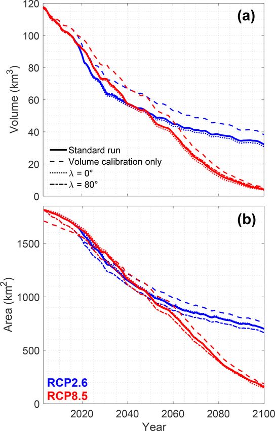
Compared to the reference simulations (with the SMB
model calibrated using glacier-specific geodetic mass bal-
ances), the simulations in which a region-wide SMB esti-
mate is used for model calibration result in a lower future
mass loss (Fig. 13, Table S4). The difference is the largest
under RCP2.6, in which the glacier volume change for the
2003–2100 period is −65 % (vs. −70 % in the standard sim-
Figure 10. Modelled volume elevation distribution in 2017 ulation). The lower mass loss results likely from the fact that
and in 2100 under various representative concentration path-
for larger glaciers the region-wide SMB estimate is typically
ways (RCPs). The values in 2100 correspond to the multi-model
mean under a specific RCP.
higher than their mass balance. By utilising region-wide esti-
mates, the mass balance is thus overestimated in general for
these glaciers that make up for a large fraction of the total
volume, resulting in a lower mass loss.
6.1.3 Role of glacier-specific geodetic mass balance
estimation
6.1.4 Simulated future climate
In this study we use direct geodetic mass balance observa-
tions from individual glaciers to calibrate the SMB model To assess the role of climate in the modelled future glacier
component. This contrasts with the original GloGEM setup state, we performed a multilinear regression analysis for cat-
(Huss and Hock, 2015), in which the calibration is based egorical data between the RCM simulation characteristics
on regional mass balance estimates. To assess the effect of (RCP, RCM, GCM and realisation) and the glacier volume
www.the-cryosphere.net/13/1125/2019/ The Cryosphere, 13, 1125–1146, 20191138 H. Zekollari et al.: Modelling the future evolution of glaciers in the European Alps Figure 11. Future evolution of the Grosser Aletschgletscher (a, b), Mer de Glace (c, d) and Langtaler Ferner (e, f) under RCP2.6 (a, c, e) and RCP8.5 (b, d, f). The 2017–2100 evolution corresponds to the multi-model mean surface evolution, while the blue area is the multi-model mean glacier geometry at the end of the century. The dotted lines represent the 2100 glacier geometries for individual RCM simulations (see Table S1). The insets represent length changes over the 2017–2100 time period for every individual RCM simulation. in 2100. In such an analysis, all independent variables are re- and finally the realisation (p = 0.13) (Table S5). This indi- placed by dummy variables, which have a value of 1 when cates that modelled future glacier evolution depends more the variable is considered, and are equal to zero otherwise strongly on the driving GCM than the RCM and that the (e.g. Liang et al., 1992; Tutz, 2012). An analysis in which realisation has a non-significant effect. The importance of all possible linear combinations are considered explains most the GCM forcing also appears from additional simulations of the variations in the 2100 volume, as the degrees of free- in which the original, low-resolution GCM output was used dom are relatively low (Table S5). An analysis of variance as model forcing. When comparing these GCM-forced sim- suggests that most of the variance is described by the RCP ulations with the corresponding GCM–RCM-forced simula- (Table S5; p value of F test < 10−3 ), as expected, and is de- tions, the rate of volume loss is slightly higher in the GCM- scribed earlier (see Fig. 8). The only other term that is sig- forced simulations in the early second part of the 21st cen- nificant at the 1 % level is the GCM (p < 10−3 ), followed by tury, but in 2100 a relatively similar glacier volume is ob- the RCM, which is significant at the 5 % level (p = 0.04), The Cryosphere, 13, 1125–1146, 2019 www.the-cryosphere.net/13/1125/2019/
You can also read