Case study of a humidity layer above Arctic stratocumulus and potential turbulent coupling with the cloud top
←
→
Page content transcription
If your browser does not render page correctly, please read the page content below
Atmos. Chem. Phys., 21, 6347–6364, 2021
https://doi.org/10.5194/acp-21-6347-2021
© Author(s) 2021. This work is distributed under
the Creative Commons Attribution 4.0 License.

Case study of a humidity layer above Arctic stratocumulus
and potential turbulent coupling with the cloud top
Ulrike Egerer1 , André Ehrlich2 , Matthias Gottschalk2,a , Hannes Griesche1 , Roel A. J. Neggers3 , Holger Siebert1 , and
Manfred Wendisch2
1 Leibniz  Institute for Tropospheric Research, Permoserstr. 15, 04318 Leipzig, Germany
2 Leipzig  Institute for Meteorology, University of Leipzig, Stephanstr. 3, 04103 Leipzig, Germany
3 Institute for Geophysics and Meteorology, University of Cologne, Pohligstr. 3, 50969 Cologne, Germany
a now at: Deutscher Wetterdienst, Frankfurter Str. 135, 63067 Offenbach, Germany

Correspondence: Ulrike Egerer (egerer@tropos.de)

Received: 11 June 2020 – Discussion started: 25 June 2020
Revised: 10 March 2021 – Accepted: 22 March 2021 – Published: 27 April 2021

Abstract. Specific humidity inversions (SHIs) above low-         ulations (LESs) complement the observations by modeling a
level cloud layers have been frequently observed in the Arc-     case of the first scenario. The simulations reproduce the ob-
tic. The formation of these SHIs is usually associated with      served downward turbulent fluxes of heat and moisture at the
large-scale advection of humid air masses. However, the po-      cloud top. The LES realizations suggest that in the presence
tential coupling of SHIs with cloud layers by turbulent pro-     of a SHI, the cloud layer remains thicker and the temperature
cesses is not fully understood. In this study, we analyze a      inversion height is elevated.
3 d period of a persistent layer of increased specific humid-
ity above a stratocumulus cloud observed during an Arctic
field campaign in June 2017. The tethered balloon system
BELUGA (Balloon-bornE moduLar Utility for profilinG the          1   Introduction
lower Atmosphere) recorded vertical profile data of meteo-
rological, turbulence, and radiation parameters in the atmo-     The Arctic atmospheric boundary layer (ABL) exhibits nu-
spheric boundary layer. An in-depth discussion of the prob-      merous particular features compared to lower latitudes, such
lems associated with humidity measurements in cloudy en-         as persistent mixed-phase clouds, multiple cloud layers de-
vironments leads to the conclusion that the observed SHIs        coupled from the surface, and ubiquitous temperature inver-
do not result from measurement artifacts. We analyze two         sions close to the surface. Local ABL and cloud processes are
different scenarios for the SHI in relation to the cloud top     complex and not completely understood, but they are con-
capped by a temperature inversion: (i) the SHI coincides         sidered an important component to explain the rapid warm-
with the cloud top, and (ii) the SHI is vertically separated     ing of the Arctic region (Wendisch et al., 2019). One of the
from the lowered cloud top. In the first case, the SHI and the   special features frequently observed in the Arctic are spe-
cloud layer are coupled by turbulence that extends over the      cific humidity inversions (SHIs), although specific humidity
cloud top and connects the two layers by turbulent mixing.       is generally expected to decrease with height (Nicholls and
Several profiles reveal downward virtual sensible and latent     Leighton, 1986; Wood, 2012). The relative frequency of oc-
heat fluxes at the cloud top, indicating entrainment of humid    currence of low-level SHIs in summer is estimated to be in
air supplied by the SHI into the cloud layer. For the second     the range of 70 %–90 % over the Arctic ocean (Naakka et al.,
case, a downward moisture transport at the base of the SHI       2018).
and an upward moisture flux at the cloud top is observed.           Arctic SHIs have been observed during past field cam-
Therefore, the area between the cloud top and SHI is sup-        paigns (Sedlar et al., 2012; Pleavin, 2013), e.g., the Surface
plied with moisture from both sides. Finally, large-eddy sim-    Heat Budget of the Arctic Ocean (SHEBA; Uttal et al., 2002)
                                                                 in 1997–1998, or the Arctic Summer Cloud Ocean Study

Published by Copernicus Publications on behalf of the European Geosciences Union.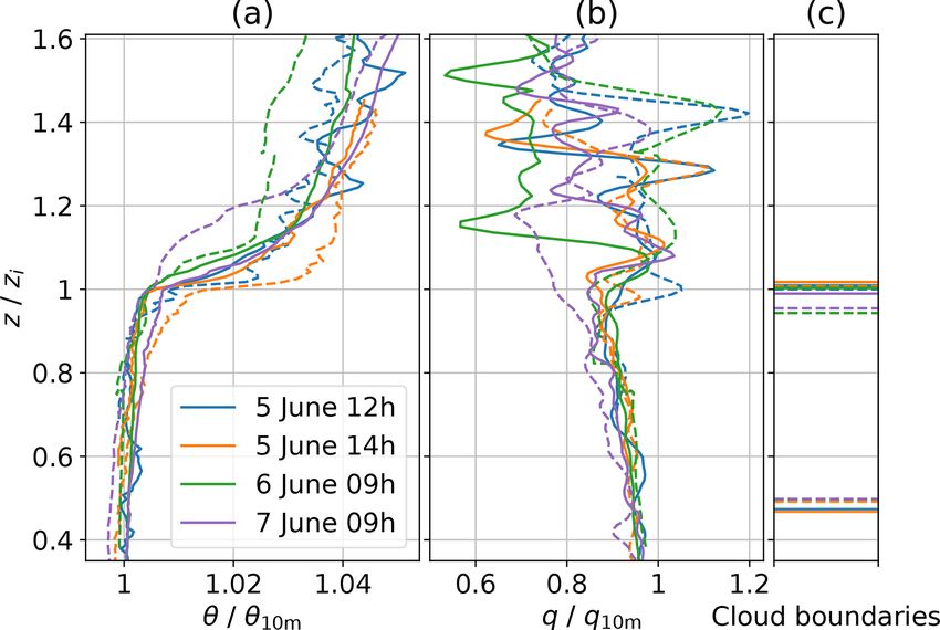
6348                                           U. Egerer et al.: Case study of a humidity layer above Arctic stratocumulus

(ASCOS; Tjernström et al., 2014) in 2008. Furthermore,               To investigate the exchange processes between the cloud
a number of studies on the climatology of SHIs have been          layer and the SHI, we performed tethered balloon-borne
published (e.g., Naakka et al., 2018; Brunke et al., 2015;        high-resolution vertical profile measurements of turbulence
Devasthale et al., 2011). SHIs occur most frequently over the     and radiation during a 3 d period in the framework of the
Arctic ocean and are strongest in summer. In the lower tro-       campaign Physical Feedbacks of Arctic Boundary Layer, Sea
posphere, they often occur in conjunction with temperature        Ice, Cloud and Aerosol (PASCAL) (Wendisch et al., 2019).
inversions and high relative humidity but are also linked to      The observations are supplemented by LES for the same pe-
the surface energy budget (Naakka et al., 2018). Formation        riod. We focus on a detailed case study with a persistent SHI
processes and interactions of SHIs with clouds have been          above a stratocumulus deck to answer the following research
investigated in large-eddy simulations (LESs). For example,       question: how are the SHI and the cloud top connected by
Solomon et al. (2014) showed that a specific humidity layer       turbulent mixing?
becomes important as a moisture source for the cloud when            The paper is structured as follows: Sect. 2 describes the ob-
moisture supply from the surface is limited. Pleavin (2013)       servations. In Sect. 3, we discuss humidity measurements in
studied how the SHIs support the mixed-phase clouds to ex-        cloudy and cold conditions and potential error sources. For
tend into the temperature and humidity inversion.                 the case study, Sect. 4 analyzes the vertical ABL structure
   Mostly, the formation of the summertime SHIs is at-            around the SHI and the relation of SHI, cloud top, and tem-
tributed to large-scale advection of humid air masses. In         perature inversion. In Sect. 5, we investigate the turbulent
the Arctic, especially over sea ice, moisture advection is        coupling between SHI and the cloud layer, and the turbulent
the critical factor for cloud formation and development           transport of heat and moisture. We close with a discussion
(Sotiropoulou et al., 2018). SHIs form when warm, moist           of the impact of the SHI on the cloud by means of LES in
air is advected over the cold sea ice surface and moisture        Sect. 6.
is removed through condensation and precipitation from the
lowest ABL part. This and further simplified formation pro-
cesses are discussed by Naakka et al. (2018).                     2     Observations
   SHIs can contribute to the longevity of Arctic mixed-phase
                                                                  2.1    The PASCAL expedition
clouds (Morrison et al., 2012; Sedlar and Tjernström, 2009),
which dominate the near-surface radiation heat budget in the      The observations analyzed in this study were performed dur-
Arctic (Intrieri et al., 2002). When a SHI is located closely     ing PASCAL (Wendisch et al., 2019), which took place in
above an Arctic stratocumulus, it can provide moisture that       the sea-ice-covered area north of Svalbard in summer 2017.
may drive the cloud evolution due to cloud top entrainment.       The RV Polarstern (Knust, 2017) carried a suite of remote
In contrast, in the typical marine sub-tropical or mid-latitude   sensing and in situ instrumentation. Additionally, an ice floe
cloud-topped ABL, dry air from above is entrained into the        camp was erected in the vicinity of the ship (Macke and Flo-
cloud (Albrecht et al., 1985; Nicholls and Leighton, 1986;        res, 2018). Knudsen et al. (2018) describe the synoptic sit-
Katzwinkel et al., 2012). However, SHIs are not well repre-       uation during the operation of the ice floe camp as climato-
sented in global atmospheric models, where the SHI strength       logically warm with prevailing warm and moist maritime air
is typically underestimated (Naakka et al., 2018), or the SHIs    masses advected from the south and east. The meteorological
are not reproduced (Sotiropoulou et al., 2016).                   conditions were influenced by a high-pressure ridge east of
   Previous studies on SHIs have been based on radiosound-        Svalbard. The present study is based on measurements with
ings, remote sensing observations, reanalysis data, or LESs.      instruments carried by the tethered balloon system BELUGA
Most observational studies rely on profiles of mean thermo-       (Balloon-bornE moduLar Utility for profilinG the lower At-
dynamic parameters from radiosoundings, which might be            mosphere; Egerer et al., 2019a). BELUGA was launched
influenced by sensor wetting after cloud penetration in the       from the sea ice floe at around 82◦ N, 10◦ E in the period
SHI region. A systematic bias in radiosonde humidity mea-         of 5–14 June 2017. The balloon measurements are comple-
surements due to sensor wetting or other error sources is a se-   mented by radiosoundings launched every 6 h (Schmithüsen,
rious concern when studying SHIs, particularly under moist        2017) and by ship-based remote sensing observations from
and cold conditions. To exclude systematic biases, one aim of     a vertical-pointing, motion-stabilized cloud radar (Griesche
this work is to carefully assess the validity of the SHI obser-   et al., 2020c), a lidar (Griesche et al., 2020b), and a mi-
vations. Due to the limited time resolution of radiosondes,       crowave radiometer of the OCEANET platform (Griesche
those measurements do not allow for turbulence observa-           et al., 2020d), which were processed with the synergistic in-
tions to analyze the exchange processes between the SHI and       strument algorithm Cloudnet (Griesche et al., 2020a).
cloud top. To date, very few data are available to character-
ize and quantify the turbulent and radiative energy fluxes at     2.2    Observation period
SHIs. However, in particular the vertical turbulent exchange
of mass and energy is necessary to understand the importance      The observational basis for this study is a persistent layer
of SHIs for cloud evolution and lifetime.                         of increased specific humidity above a single-layer stratocu-

Atmos. Chem. Phys., 21, 6347–6364, 2021                                             https://doi.org/10.5194/acp-21-6347-2021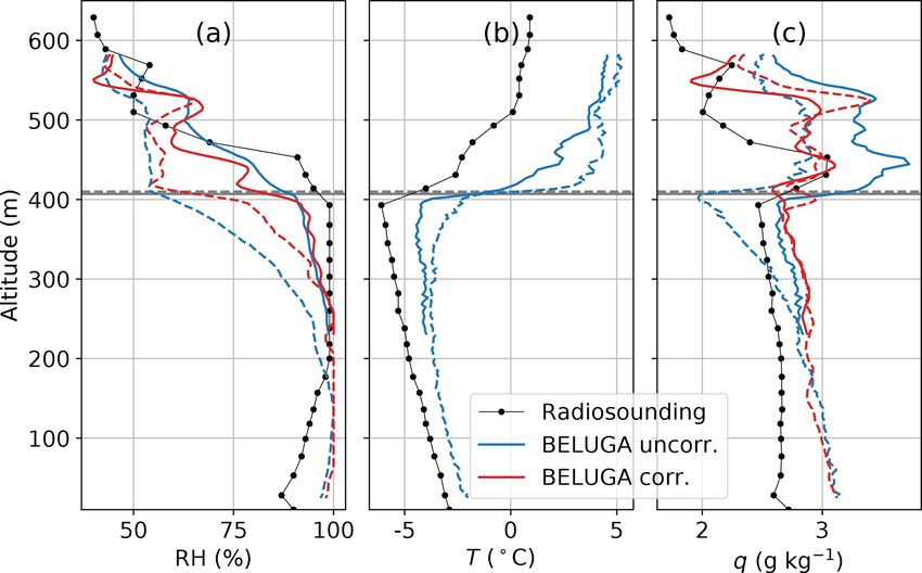
U. Egerer et al.: Case study of a humidity layer above Arctic stratocumulus 6349
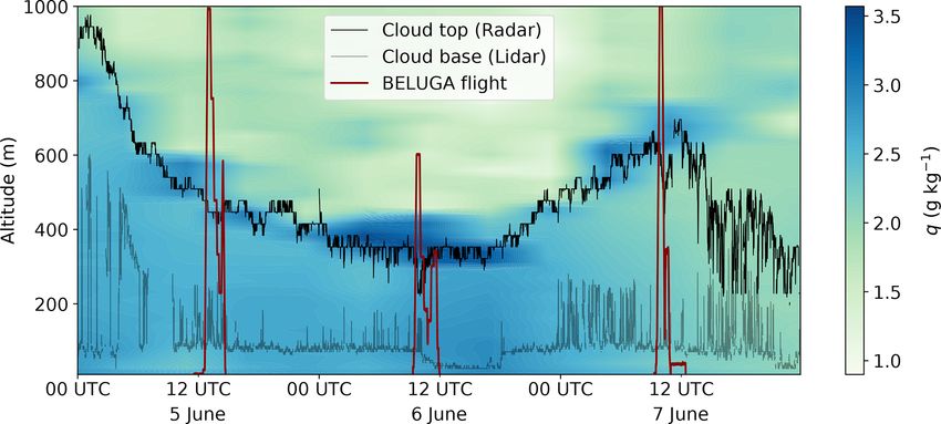
Figure 1. Temporal development of the specific humidity vertical profile observed by radiosondes. The radar-retrieved cloud top height is
depicted as a black line; the cloud base height derived from the lidar near-field channel is indicated as a grey line. The red lines represent the
BELUGA flight profiles.
mulus deck during the period between 5 and 7 June 2017. packages to explore the ABL between the surface and 1500 m
Figure 1 illustrates the temporal development of the vertical altitude. BELUGA can operate under cloudy and light icing
specific humidity profile derived from radiosonde measure- conditions in the Arctic. Fixed to the balloon tether, a fast
ments. Cloud top and bottom and the time–height curves of (50 Hz resolution) ultrasonic anemometer, supported by an
the corresponding BELUGA flights are added for the inves- inertial navigation system, measures the wind velocity vector
tigated period. The BELUGA flights were conducted around in an Earth-fixed coordinate system together with the sonic
noon on each of the three consecutive days. A local maxi- temperature. Especially at low specific humidity, the sonic
mum of specific humidity is observed above the cloud top temperature is close to the virtual temperature, which will be
throughout almost the entire period, with a slight diurnal cy- used in the following. Furthermore, barometric pressure, rel-
cle peaking at noon and a maximum specific humidity on ative humidity, and the static air temperature are measured
6 June. It is worth noting that the observations show a well- with lower resolution (1 Hz). Relative humidity (RH) is mea-
defined layer of increased specific humidity, hereafter re- sured with a capacitive humidity sensor. The housing of the
ferred to as the humidity layer, rather than a distinct and sharp RH sensor, which has a high diffusivity for water vapor, also
SHI with only a slight decrease above. accommodates a temperature sensor for the sensor-internal
The cloud top and base height in Fig. 1 are estimated from temperature. The air temperature is measured with a PT100
the cloud radar and lidar (near-field channel) data, averaged for reference and a thermocouple for temperature fluctua-
over 30 s and with a vertical resolution of 30 m. Through- tions (at 50 Hz). A second instrument payload is fixed simul-
out the 3 d period, cloud height and thickness decrease to a taneously to the tether, measuring broadband terrestrial and
minimum at noon of 6 June and thereafter increase again. solar net irradiances. Technical details on BELUGA, its in-
The cloud is almost permanently of mixed-phase type with strumentation, and operation during PASCAL as well as data
a maximum liquid water content (LWC) between 0.15 and processing methods are given by Egerer et al. (2019a).
0.6 g m−3 and an estimated ice water content (IWC) of about
0.03 g m−3 derived from Cloudnet data (not shown here).
Figure 1 depicts the high variability in cloud top and bot- 3 Specific humidity measurements in a moist
tom heights. To illustrate the cloud situation around the BEL- environment
UGA flights in more detail, Fig. 2 shows the radar reflectivity
A cold and moist environment poses considerable challenges
and cloud boundaries for the particular three balloon flights.
for the measurement of specific humidity. This can lead to
On 5 June, the cloud top height is approximately constant,
measurement artifacts in the region of the SHI. Therefore, in
whereas on 6 June the cloud top fluctuates between 350 and
this section we discuss the measurement of specific humidity
230 m in the course of the flight. During the 7 June flight, the
with BELUGA and radiosondes as well as possible sources
cloud layer thins by 110 m starting from the cloud top.
of error and their effects. Specific humidity q is derived from
air temperature T and RH using
2.3 BELUGA setup
Rd /Rv · es (T ) · RH
q= , (1)
The BELUGA system consists of a 90 m3
helium-filled teth- p − (1 − Rd /Rv ) · es (T ) · RH
ered balloon with a modular setup of different instrument
https://doi.org/10.5194/acp-21-6347-2021 Atmos. Chem. Phys., 21, 6347–6364, 2021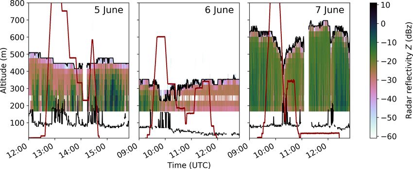
6350                                                U. Egerer et al.: Case study of a humidity layer above Arctic stratocumulus

Figure 2. BELUGA flight profiles for 5, 6, and 7 June (red lines) with the radar reflectivity Z and cloud boundaries (black lines, as in Fig. 1).

with the static pressure p, the ratio of specific gas con-                  iii. Furthermore, the time response for RH and T measure-
stants of dry air and water vapor Rd /Rv ≈ 0.622, and the                        ments is finite. Compared to the effects (i) and (ii), this
temperature-dependent saturation vapor pressure es (T ). In                      part of the sensor behavior can be quantified by the time
this study, the measurements of RH and T are obtained                            constant τ . Assuming a first-order sensor response, the
by regular radiosoundings (Vaisala RS92-SGP) and ob-                             time dependence of a measured signal xm (t) (RH or T
servations with the BELUGA system. Both methods use                              in our case) is given by
capacitive RH sensors, suffering from several limitations
(Wendisch and Brenguier, 2013).                                                  dxm
                                                                                     = 1/τ (xa − xm ) ,                                      (2)
                                                                                  dt
3.1    Error sources for humidity measurements
                                                                                 with the e−1 time constant τ and the ambient (“true”)
Several studies address the associated systematic errors of                      signal xa .
radiosonde RH and T measurements and identify three main                         The time-lag-corrected signal is
sources, (i) wet-bulbing, (ii) solar heating, and (iii) time re-
                                                                                       x̃m (t) − x̃m (t − 1t) · e−1t/τ

sponse errors:
                                                                                 xτ =                                    ,                   (3)
                                                                                                  1 − e−1t/τ
  i. Wet-bulbing occurs when a water film develops on the
     sensor during cloud penetration, with subsequent evapo-                     with 1t being the time step between two consecutive
     rative cooling under sub-saturated conditions above the                     measurement points (Miloshevich et al., 2004). Here,
     cloud. This effect leads to an overestimation of RH and                     we assume that the time-corrected value (index τ ) is
     underestimation of T in the sub-saturated environment                       equal to the ambient value xa . The tilde in Eq. (3) rep-
     until the water film has completely evaporated. Jensen                      resents the low-pass-filtered, measured time series.
     et al. (2016) show that wet-bulbing is an issue for the ra-
                                                                              Although radiosonde data processing routines consider the
     diosonde type used during PASCAL. However, the error
                                                                           time response error, fast humidity changes in cold conditions
     induced by wet-bulbing is difficult to quantify (Dirksen
                                                                           are still affected (Smit et al., 2013; Edwards et al., 2014). The
     et al., 2014).
                                                                           time constants for the BELUGA RH sensor were estimated
 ii. Exposure of an RH sensor to direct sunlight above a                   in a laboratory study (see Appendix A) and are τRH ≈ 50 s
     cloud causes a radiation dry bias (measured RH is too                 for RH and τTs ≈ 70 s for the internal temperature. The time
     low) of up to 5 % in the lower troposphere (Miloshevich               constant for the T measurements based on the thermocouple
     et al., 2009; Wang et al., 2013). The error is corrected in           on BELUGA was found to be below 1 s (Egerer et al., 2019a)
     the radiosonde data processing algorithm (Jensen et al.,              and, thus, has a minor influence on the vertical temperature
     2016). However, this correction is intended for cloud-                profile compared to the humidity observations.
     free conditions. Solar heating also influences tempera-
     ture measurements (Sun et al., 2013), but the effect on               3.2   Sensitivity of q to the RH and T profile
     radiosonde temperature is negligible at low altitudes.
                                                                           We perform sensitivity studies to analyze how the three error
     For BELUGA, the temperature and RH sensors are
                                                                           sources (cf. Sect. 3.1) for T and RH measurements combine
     shielded against direct solar radiation, but the sensor
                                                                           and influence the derivation of q. The errors are simulated as
     surroundings might warm and influence the measure-
                                                                           T and RH deviations from a synthetic reference case (grey
     ments.
                                                                           line in Fig. 3), which represents a simulated measurement

Atmos. Chem. Phys., 21, 6347–6364, 2021                                                       https://doi.org/10.5194/acp-21-6347-2021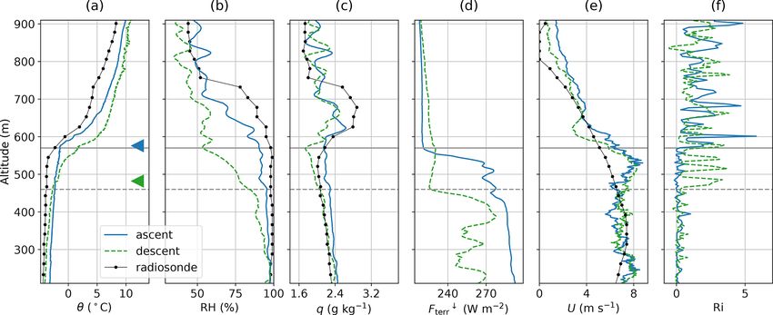
U. Egerer et al.: Case study of a humidity layer above Arctic stratocumulus                                                           6351

                                                                          vertical structure shifts upwards or downwards for an ascent
                                                                          or descent. With a slow-response RH sensor (τRH  τT ), the
                                                                          measured RH in the SHI region is overestimated on the as-
                                                                          cent and underestimated on the descent with the effects on q
                                                                          as shown in Fig. 3c and with an artificial SHI on the ascent.
                                                                             As a result of these sensitivity studies, the error in q is re-
                                                                          duced when both the temperature and humidity sensors are
                                                                          affected by the same error source (e.g., solar heating on both
                                                                          sensors), and when both sensors have comparable time con-
                                                                          stants. Under these conditions, a detected SHI can be consid-
                                                                          ered as most likely real and does not need to be interpreted
                                                                          as an artifact.

                                                                          3.3   SHIs measured with BELUGA and radiosondes:
Figure 3. Sensitivity of the vertical q profile to a deviation of T and         natural feature or artifact?
RH compared to a reference case (grey line). Only one parameter (T
or RH) experiences a deviation in the inversion region, the other pa-
                                                                          A simple and convincing test of the possible influence of the
rameter is unchanged. Underestimated temperature (blue) or over-
estimated RH (green) might result from wet-bulbing. Overestimated         error sources on the SHI observations is profiling in opposite
temperature (purple) or underestimated RH (orange) might result           direction, that is a descent from the free troposphere through
from solar heating. A slow-response RH sensor overestimates RH            the SHI into the cloud layer. This is commonly impossible
on the ascent (green) and underestimates RH on the descent (or-           in case of standard radiosoundings, but feasible for the BEL-
ange).                                                                    UGA observations. Figure 4 shows vertical profiles of RH,
                                                                          T , and q as measured by radiosounding and BELUGA on
                                                                          5 June 2017. Qualitatively, the measurements of both plat-
of a temperature inversion combined with a decrease in RH.                forms show a similar vertical structure with a sharp temper-
The temperature linearly increases by 6 K in the 200 m thick              ature inversion capping the cloud layer. The cloud top (es-
inversion layer, whereas RH linearly decreases from 100 %                 timated from the observed downward terrestrial irradiance)
to 40 % in the same height range, resulting in monotonically              is situated close to the temperature inversion base. How-
decreasing specific humidity without a SHI.                               ever, the cloud top height derived from radiation observa-
   First, we consider the influence of possible measurement               tions should be treated with caution due to the vertical sepa-
errors in the temperature inversion region for the T and RH               ration of the radiation and thermodynamic sensors by about
sensor separately. That is, only one sensor will be influenced            20 m, corresponding to a temporal shift between the obser-
by an increased or decreased signal while keeping the other               vations of about 20 s during profiling. In the course of the
sensor reading at the reference value.                                    measurement period of almost 2 h, the temperature inversion
   The magnitude of the simulated deviations (Fig. 3a and b)              base and the cloud top remain at almost constant altitude.
is arbitrary, but the qualitative profile of the affected signal is       The radiosonde observation shows a layer of increased q be-
according to the error sources, as discussed in Sect. 3.1.                tween 400 and 550 m altitude just above the temperature in-
   The effect of the four errors (T or RH too high or too low             version base. The increased specific humidity emerges from
in the temperature inversion region) on the specific humidity             RH remaining high within the temperature inversion, before
profile is shown in Fig. 3c. An artificial humidity layer above           decreasing to the free troposphere level well above the inver-
the cloud can emerge when the RH sensor overestimates the                 sion base.
moisture due to wet-bulbing (but keeping the temperature                     Before comparing the q measurements from the ra-
sensor unaffected), or when the temperature sensor is heated              diosonde to BELUGA observations, we illustrate the effect
in the inversion region but the humidity sensor is unaffected.            of the applied RH correction and the consequences for the q
Vice versa, q shows a deficit compared to the reference when              profile. Figure 4a shows the uncorrected and time-response-
one of the sensors indicates underestimated values compared               corrected RH for an ascent and descent. The uncorrected RH
to the reference scenario. If a single phenomenon affects both            ascent profile deviates strongly from the descent in the cloud
the temperature and RH sensor (e.g., solar heating results in             top region. While descending through the cloud, the sensor
underestimated RH and overestimated temperature), the er-                 requires a 150 m height difference for rising from 55 % to
rors in the determination of q have an opposite effect and,               95 % RH. The RH hysteresis around the cloud top is visi-
therefore, the overall error in q is reduced.                             ble as a systematic deviation in all observed flight data (not
   As a second step, we simulate the influence of different               shown). A comparison to Fig. 3 (orange lines) suggests that
time constants τRH and τT for the RH and temperature mea-                 the major part of the error is due to a slow RH sensor. Fur-
surements. If both time constants have similar values, the re-            thermore, the sensor underestimates RH in the cloud on the
sulting q does not change significantly in magnitude, but the             descent, which might indicate solar heating. After applying

https://doi.org/10.5194/acp-21-6347-2021                                                   Atmos. Chem. Phys., 21, 6347–6364, 2021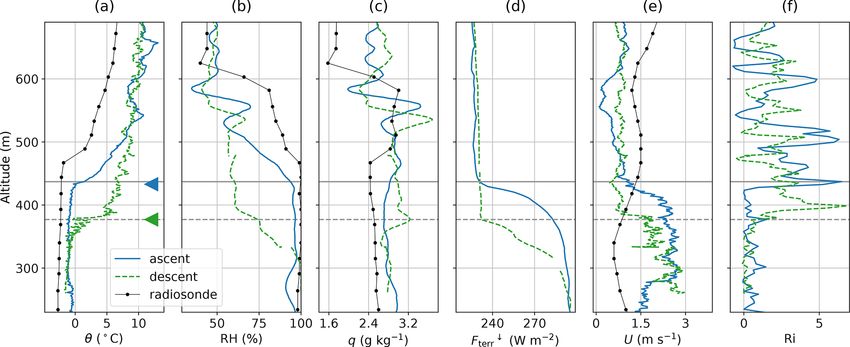
6352                                              U. Egerer et al.: Case study of a humidity layer above Arctic stratocumulus

Figure 4. Vertical profiles of (a) relative humidity RH, (b) tem-
perature T , and (c) specific humidity q measured by a radiosonde    Figure 5. Balloon-borne vertical profiles of (a) potential tempera-
and BELUGA on 5 June 2017 (second profile). RH and q for BEL-        ture θ, (b) specific humidity q, and (c) cloud boundaries for four
UGA are shown before and after the corrections. The radiosonde       ascents (solid lines) and descents (dashed lines) on 5, 6, and 7 June
was launched at 16:50 UTC; the balloon flew a continuous ascent      2017. The altitude z is normalized to the temperature inversion base
and descent from 14:15 to 14:40 UTC. The cloud top (from BEL-        height zi . Potential temperature θ and the specific humidity q are
UGA radiation data) is shown as horizontal lines. Solid and dashed   normalized to their near-surface values. The cloud top is derived
lines represent the BELUGA ascent and descent, respectively.         from the irradiance profile; the cloud base is derived from Cloudnet
                                                                     data. The profiles are named after the start time (cf. Fig. 2).

the time lag correction, the RH profile shows a significantly
                                                                     ence of solar heating and time-lag errors is minimized. Our
reduced difference between ascent and descent. The remain-
                                                                     conclusion also strengthens the confidence in SHIs as fre-
ing difference is qualitatively consistent with the temperature
                                                                     quently observed by radiosondes.
observations as shown in Fig. 4b. The temperature profiles
show a warming of the cloud top and inversion region be-
tween 300 and 500 m during the descent leading to a reduced          4     Vertical profiles of mean ABL parameters
RH.
   The “uncorrected” specific humidity in Fig. 4c is calcu-          4.1    Comparison of normalized temperature and
lated from the uncorrected RH and the temperature measured                  humidity profiles
with the fast-response thermocouple. The resulting q profiles
show a SHI on the ascent and the descent of the BELUGA               Throughout the observation period, we observe a persistent
flight with a similar structure and location compared to the         layer of increased specific humidity above the cloud layer.
radiosonde data. The q profile as observed during the descent        One of the governing questions of this analysis is to under-
is shifted to lower q values in the region of the hysteresis of      stand how observed SHIs relate to the general ABL structure
the uncorrected RH.                                                  and, in particular, to the temperature inversion. Figure 5a and
   The corrected q results from the RH and the sensor-               b shows vertical profiles of potential temperature θ and spe-
internal temperature Ts after correcting both signals for the        cific humidity q recorded in the period of 5–7 June 2017.
time lag error according to Eq. (3). We argue that using Ts          Both parameters are normalized to their near-surface values
should be preferred instead of the thermocouple readings be-         and plotted in relation to the base height of the temperature
cause RH and Ts have similar time constants, and RH is mea-          inversion zi . The cloud boundaries are shown in Fig. 5c for
sured at Ts instead of the temperature of the atmospheric en-        reference.
vironment. The ambient temperature and Ts differ slightly               All measurements show a similar vertical structure of θ
due to the thermal inertia of the sensor housing.                    within the ABL. Below the temperature inversion base zi ,
   After applying the corrections, the maximum value of the          the stratification is near-neutral to weakly stable. Above
SHI, as observed during the BELUGA ascent, is reduced by             the inversion, the thermodynamic stability is higher and ex-
about 0.6 g kg−1 compared to the uncorrected q maximum.              hibits more variability compared to below the inversion. No
After correction, all BELUGA profiles and the radiosonde             systematic difference between ascents and descents is visi-
data exhibit the SHI with similar structure and amplitude.           ble. The ABL is thermodynamically coupled to the surface,
This consistency suggests that the observed SHI is a natural         which makes normalizing to surface values meaningful.
feature instead of an instrumental artifact. We can exclude             Within the mixed layer below zi , specific humidity de-
wet-bulbing as the main reason for the observed SHIs be-             creases slightly with height but increases when reaching zi .
cause the SHI is also present during the descent. The influ-         Above zi , the normalized specific humidity exhibits more

Atmos. Chem. Phys., 21, 6347–6364, 2021                                                 https://doi.org/10.5194/acp-21-6347-2021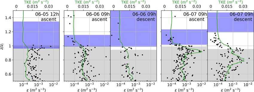
U. Egerer et al.: Case study of a humidity layer above Arctic stratocumulus                                                             6353

Figure 6. Boundary layer observations around the cloud top on 5 June 2017, first profile: vertical profiles of (a) potential temperature θ ,
                                                                       ↓
(b) RH, (c) specific humidity q, (d) downward terrestrial irradiance Fterr , (e) horizontal wind velocity U , and (f) Richardson number Ri for
BELUGA ascent and descent and the radiosonde launched at 11:00 UTC. The triangles indicate where zi is defined. The cloud top is shown
as horizontal lines (solid for ascents and dashed for descents).

variability compared to the normalized temperature. The de-              Richardson number Ri as measured during ascents and de-
scent of 7 June 09 h shows a temperature inversion with some             scents on 5, 6, and 7 June, respectively. We analyze only con-
internal structure in the form of two smaller “steps” in θ . We          tinuous profile data without longer breaks at certain heights
define zi at the lower step, with the SHI base being located             for the first profile of each day. The cloud top height is de-
                                                                                                              ↓
clearly above at the upper step at z ≈ 1.2 · zi . For this case,         fined by the discontinuity of the Fterr profile and marked with
a deficit in q is observed below the SHI, which is plausible             horizontal lines, whereas zi is indicated with triangles. The
because between ascent and descent cloud top had decreased               Richardson number is the ratio between thermodynamic sta-
to about 0.95 · zi .                                                     bility and wind shear and, therefore, a measure for the ability
   For most profiles, the cloud top coincides with zi , and the          of turbulence generation (Ri . 1) or dissipation (Ri & 1).
increased humidity is observed above the cloud layer. Only                  On 5 June (Fig. 6), zi lowers from 430 to 380 m in
for two profiles (both descents on 5 June), the lower bound of           the course of the BELUGA flight. The temperature differ-
the SHI is already located below the cloud top. We do not find           ence across the inversion of 1θ ≈ 9 K, which is also the
clouds penetrating into the temperature inversion, although              strongest observed during our flights, stays constant during
such situations have been frequently observed in previous                ascent and descent. The RH decreases within the tempera-
studies (e.g., Pleavin, 2013; Sedlar et al., 2012; Sedlar and            ture inversion, accompanied by an increase in q above zi of
Shupe, 2014; Shupe et al., 2013; Brooks et al., 2017). How-              about 0.25 g kg−1 (ascent) and 0.5 g kg−1 (descent). The ra-
ever, two of the descent profiles (6 June 09 h and 7 June 09 h)          diosonde, launched around 2 h prior to the BELUGA flight,
show situations where the cloud top had decreased between                shows a higher zi but qualitatively a similar vertical structure
ascent and descent, and the SHI is vertically separated from             of θ , RH, and q. The cloud top agrees well with zi for the as-
the cloud top.                                                           cent and descent. The horizontal wind velocity U is around
                                                                         2 m s−1 inside the cloud layer and decreases to 1 m s−1 in the
4.2   Cloud top variability versus SHI height                            free troposphere, resulting in horizontal wind shear. During
                                                                         the ascent, the wind shear zone is clearly located below zi
The cloud top variability, here defined as the cloud top height          with a sudden increase in Ri to values greater than 1 above
difference between ascent and subsequent descent for each                zi and cloud top. During the descent, the strongest wind
profile, is related to zi and the lower boundary of the SHI. For         shear is observed around zi , and the resulting increase in
all 3 d, a descending cloud top is observed between the ascent           Ri is slightly above zi . This vertical shift suggests a slightly
and subsequent descent with a cloud top height difference of             stronger turbulent coupling between cloud top and the SHI
50 to 100 m. This cloud top variability is indicated by in situ          above, as compared to the ascent.
irradiance and thermodynamic measurements and also con-                     The general ABL structure observed on 6 June (Fig. 7) in
firmed by radar reflectivity (cf. Fig. 2). In order to illustrate        terms of the profiles of θ , RH, and q is quite similar to the
the relation of cloud top height, SHI, and other ABL param-              5 June observations, showing a decreasing cloud top height
eters, Figs. 6–8 show profiles of mean θ , RH, q, downward               during the balloon operation. Here, zi decreases from 290 m
                           ↓
terrestrial irradiance Fterr , horizontal wind velocity U , and

https://doi.org/10.5194/acp-21-6347-2021                                                    Atmos. Chem. Phys., 21, 6347–6364, 2021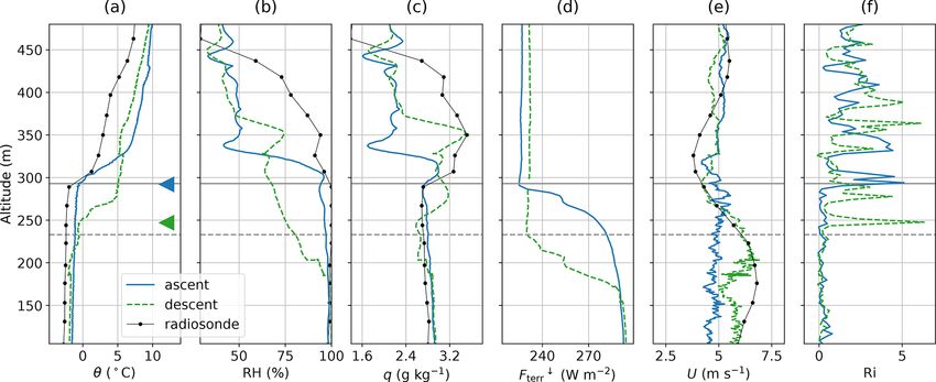
6354                                                 U. Egerer et al.: Case study of a humidity layer above Arctic stratocumulus

Figure 7. Same as Fig. 6, but for 6 June 2017 (first profile).

during the ascent to about 230 m during the descent. The ra-           the SHI base are separated by 110 m on the descent. The ter-
diosonde, launched 1.5 h after the BELUGA flight, shows a              restrial irradiance inside the cloud layer fluctuates strongly,
similar zi to the balloon ascent, indicating that zi and cloud         especially on the descent, which suggests a patchy cloud
top recover between BELUGA descent and radiosounding.                  with cloud holes. The horizontal wind velocity agrees quali-
This is in agreement with the radar observations in Fig. 2.            tatively for all three profiles. Inside the ABL, a higher wind
The lower bound of the SHI with 1q ≈ 0.3 g kg−1 on the as-             velocity of around 6 m s−1 is observed with the BELUGA
cent and 0.7 g kg−1 on the descent is coupled to zi in both            observations, showing a local maximum of 8 m s−1 slightly
cases. On the ascent, zi coincides with the cloud top. Dur-            below zi . Above this maximum, U gradually decreases to
ing the descent, the cloud top is almost 20 m below zi , which         2 m s−1 in the free troposphere. According to the Richardson
could possibly result from cloud top heterogeneity. However,           number, wind shear limits turbulence above the cloud top for
the temperature gradient is smoother compared to the ascent,           both ascent and descent.
which leads to a less clear determination of zi . The humidity            To resume, we observed mean profiles of several cases
structure above the cloud layer observed by the radiosonde             where cloud tops coincide with zi and the SHI base. Al-
exhibits a distinct SHI with a lower bound coupled to the              though some cloud tops show more or less strong horizontal
temperature inversion. Peak values of q are comparable with            wind shear, the stabilizing effect of the temperature inversion
BELUGA observations made during the descent. The hor-                  leads to a sudden increase in Ri just above the cloud layer,
izontal wind velocity is about 5 m s−1 and almost height-              which suggests a rather low turbulent exchange with the hu-
constant for the entire ascent but increases by about 2 m s−1          midity layers above. However, for one case a special situation
inside the cloud layer during the descent. The radiosonde              provides a new aspect of this phenomenon: zi and cloud top
provides a similar picture to the balloon descent. For the as-         height had decreased while the humidity layer remained at
cent, the sharp increase in Ri is connected to zi , whereas for        its vertical position, leading to a humidity gap between cloud
the descent this increase in Ri is – similar to the previous           top and SHI.
day – about 20 m above cloud top, allowing for some turbu-
lent exchange between the cloud and the SHI above.
   On 7 June, a clear SHI develops with a lower boundary               5   Turbulence at cloud top and around the SHI
at around 580 m, which is similar in the two BELUGA and
                                                                       Concerning the question of how the humidity and cloud layer
the radiosonde profiles (Fig. 8). For the BELUGA ascent and
                                                                       interact and to what extent these layers exchange energy by
the radiosonde profile, this boundary agrees well with zi and
                                                                       turbulent transport, we first describe the interface between
cloud top (for the radiosonde data cloud top can be roughly
                                                                       the SHI and cloud top by means of observations at constant
estimated from the RH profile). The radiosonde profile and
                                                                       altitude (Sect. 5.1). We then analyze the vertical profiles of
BELUGA ascent are shifted in time by about 70 min and
                                                                       basic turbulence parameters (Sect. 5.2) and turbulent energy
the remarkable match in zi should not be over-interpreted.
                                                                       fluxes (Sect. 5.3).
For the BELUGA descent, the thermal stratification changes
again (similar to the previous days). The temperature inver-
sion weakens and zi is shifted downward by about 110 to
480 m, together with the cloud top. Thus, the cloud top and

Atmos. Chem. Phys., 21, 6347–6364, 2021                                                 https://doi.org/10.5194/acp-21-6347-2021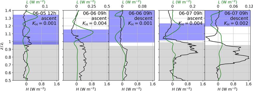
U. Egerer et al.: Case study of a humidity layer above Arctic stratocumulus                                                         6355

Figure 8. Same as Fig. 6, but for 7 June 2017.

                                                                        ture gradient (Fig. 7), the changes in θv would correspond
                                                                        to a height variation of ∼ 10 m. More likely, parts of the
                                                                        height-constant measurements (1z ≈ 1 m) are taken in po-
                                                                        tentially colder, drier, and more turbulent air masses at the
                                                                        inversion base, interrupted by measurements in potentially
                                                                        warmer, more humid, and less turbulent air masses at higher
                                                                        altitudes well within the T inversion. This variability is also
                                                                        visible in the wind direction (not shown here). Depending
                                                                        on the relative location of zi to the measurement height, the
                                                                        co-variance w 0 θv0 is highly intermittent and no mean flux is
                                                                        derived from these observations.
                                                                           The center part of the record is characterized by a compa-
                                                                        rably low variability leading to the conclusion that this part of
                                                                        the observations is performed entirely inside the descending
                                                                        temperature inversion. Finally, observations are performed
                                                                        well above zi inside the stably stratified T inversion layer,
                                                                        characterized by values of ε 1 order of magnitude lower com-
Figure 9. Constant-altitude time series of (a) virtual potential tem-   pared to at the inversion base. Here, variations in θv and q are
perature θv , (b) specific humidity q, (c) vertical wind w, (d) co-     again correlated and caused by changes in relative height.
variance θv 0 w0 , and (e) dissipation rate ε for 6 June measured at       The observations do not allow for drawing quantita-
300 m altitude around zi .
                                                                        tive conclusions, such as time and area-averaged turbulent
                                                                        heat fluxes, from this record. However, these measurements
                                                                        vividly illustrate the difficulties in estimating turbulent fluxes
5.1   Observations at constant altitude in the inversion                based on covariance methods in the vicinity of the tempera-
      layer                                                             ture inversion, although the measurement height is kept at a
                                                                        remarkably constant height level. Therefore, the methods for
To get an insight into the transition from cloud top to the             estimating turbulent fluxes based on mean vertical gradients
humidity layer above, measurements were taken at a constant             and slant profiles are more suitable for this study and are used
height in the temperature inversion region. Figure 9 shows a            below.
500 s time series measured on 6 June at a constant altitude
around zi ≈ 300 m (second last constant altitude segment in             5.2   Vertical profiles of turbulent energy and dissipation
Fig. 2 for 6 June). The local dissipation rate ε is evaluated in
2 s segments to illustrate the evolving turbulence intensity.           The vertical distribution of turbulence parameters, such as lo-
   Within the first third of the record, the virtual potential          cal dissipation rate ε and the turbulent kinetic energy TKE,
temperature θv (as approximately measured by the ultrasonic             provide an insight into the coupling between the cloud layer
anemometer) shows strong variations on a typical timescale              and the SHI. The local ε values are derived from second-
of 30–50 s with amplitudes up to 3 K. Based on the tempera-             order structure functions by applying inertial subrange scal-

https://doi.org/10.5194/acp-21-6347-2021                                                 Atmos. Chem. Phys., 21, 6347–6364, 2021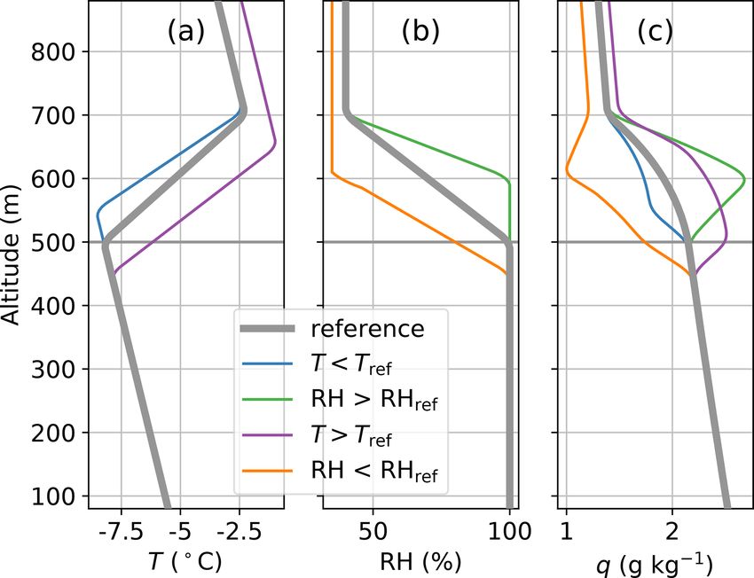
6356                                               U. Egerer et al.: Case study of a humidity layer above Arctic stratocumulus

Figure 10. Vertical profiles of local dissipation rate ε and TKE for the first ascent and descent of 5, 6, and 7 June 2017. The height is
normalized by the temperature inversion base zi . The region of increased specific humidity is marked as blue shading, the cloud layer as grey
shading.

ing as described by Egerer et al. (2019a). Different from that           tions that require further observations and a more detailed
study, here ε is calculated from non-overlapping, 2 s sub-               LES analysis.
records yielding a vertical resolution of about 2 m. Regions
without inertial sub-range scaling are excluded. Turbulent ki-           5.3    Vertical profiles of turbulent moisture and heat
netic energy (= 0.5 · u2i ) is calculated in a moving 50 s win-                 fluxes
dow. The observed TKE noise level is about 0.005 m2 s−2
and is usually reached at z/zi & 1.1.                                    The turbulent exchange of moisture can be quantified by the
   Figure 10 shows ε and TKE for each first profile of 5, 6,             latent heat flux
and 7 June as a function of normalized height (the descent of
5 June is excluded due to data issues). The cloud and humid-             L = ρ · Lv · w0 q 0 ,                                            (4)
ity layers are shaded for reference. For the presented cases,
                                                                         whereas the virtual sensible heat flux is given by
turbulence is most pronounced in the upper cloud layer and
around cloud top with typical values of ε ∼ 10−3 m2 s−3 and              H = ρ · cp · w 0 θv0 ,                                           (5)
TKE ∼ 0.02 m2 s−2 . For 5 and 6 June, the turbulence inten-
sity is rather constant in the cloud. For 7 June, with increased         with an overline describing an average of the sub-record.
wind velocity, a maximum of ε is evident just below cloud                Here, ρ is the mean air density, Lv = 2.5 × 10⁶ J kg−1 is the
top.                                                                     latent heat of evaporation, and cp = 1005 J kg−1 K−1 is the
   Figure 10 also illustrates how the SHI and cloud layer are            specific heat capacity of air. This direct calculation of H
either separated or overlap, and how they are connected by               and L requires sufficient long, stationary, and homogeneous
turbulent motion. At a certain height level, ε decreases to              records in a certain height to provide time-averaged esti-
the low-turbulence free-troposphere level. The transition is             mates of the covariances with statistical significance (Stull,
gradual, indicating turbulent mixing in this region. On 5 June           1988; Lenschow et al., 1994). Our observations focus mainly
and the ascents of 6 and 7 June, the SHI and the cloud are               on vertical profiling, and only a limited number of height-
directly coupled by turbulent mixing. For the descents of 6              constant records around the cloud top and inversion region
and 7 June, most of the mixing takes place at the interface of           are available. As shown in Sect. 5.1, the conditions around
the cloud top with the humidity gap between cloud and SHI.               the temperature inversion are highly instationary and, thus,
In this case, inside the SHI the turbulence intensity is reduced         we use the vertical profiles to study the fluxes in this region.
almost to the free-troposphere level and the SHI seems to                We apply two approaches for estimating fluxes from vertical
be decoupled from the cloud layer via the humidity gap in                profiles: (i) describing the flux profile by applying the so-
between.                                                                 called “slant profile method” and (ii) relating the turbulent
   We can only speculate about the reason for the develop-               flux to mean gradients (flux gradient method).
ment of this humidity gap, which is most pronounced for the                 The slant profile method is based on the assumption that
descent of 7 June. One explanation could be long-range ad-               for a certain height range the profile data are considered as
vection of increased moisture in the free troposphere com-               a homogeneous record and Eq. (5) can be applied. For this
bined with a temporary collapse of the well-mixed cloud                  method, instantaneous values of H are estimated for a de-
layer leading to a vertical separation of cloud top and SHI.             fined height range, defining also the length scales contribut-
However, this interesting feature leads to new research ques-            ing to the flux. For our observations, this method provides

Atmos. Chem. Phys., 21, 6347–6364, 2021                                                      https://doi.org/10.5194/acp-21-6347-2021
U. Egerer et al.: Case study of a humidity layer above Arctic stratocumulus 6357
Figure 11. Same as Fig. 10, but for the virtual sensible heat flux H (eddy covariance method) and the latent heat flux L (flux gradient
method).
only results for H due to the lack of fast-response humid- (H > 0), most pronounced for the last two profiles with a lo-
ity measurements. Alternatively, L can be estimated with the cal maximum between 0.8 < z/zi < 1. Only for the first as-
flux gradient method. This method is based on the relation cent of 5 June is the H flux almost height-constant with much
between the covariances and the mean gradients of θv and q: lower values compared to the other days. For this day, θv ex-
hibits larger variability around and slightly above zi , which
∂θ v differs from the typical structure of a turbulent flow. This
w0 θv0 = −KH · , (6)
∂z variability mainly causes the positive values of H around zi ,
which, therefore, should not be misinterpreted. This is a sim-
and ilar effect to that discussed in Sect. 5.1. A negative peak of H
around or slightly above zi is visible for the descent of 6 June
∂q
w0 q 0 = −KQ · , (7) and both profiles of 7 June. On 7 June, a secondary, weaker
∂z negative peak in H is located at the lower part of the SHI.
with KH and KQ being the turbulent exchange coefficients Although it is known that in general K = K(z), we esti-
for sensible and latent heat, respectively. The coefficients are mate a constant KH for each ascent and descent in the lower
defined as positive, which means that the flux is directed region of the SHI, which is the focus area of our study. In that
against the mean gradient. Values of K can be derived from region, we observe negative H fluxes and positive θv gradi-
parameterizations based on turbulence observations such as ents. Applying Eq. (6) leads to mean values of KH between
proposed by Hanna (1968) or by directly applying Eq. (6) 0.001 and 0.004 m2 s−1 for the five profiles. The KH (= KQ )
with the measured H , yielding KH . With KQ ≈ KH (Dyer, values for each profile are used for calculating the L profile
1967) for a wide range of stratification and the mean humid- based on the flux gradient method.
ity gradient ∂q/∂z, we estimate L by combining Eqs. (7) and A negative peak in L is observed for all days in the lower
(4). SHI region. The downward energy flux at cloud top is com-
Before estimating H from the slant profiles by applying mon for the entrainment region, where potentially warmer
Eq. (5), the turbulent fluctuations must be determined. This is and usually drier air from the free troposphere is mixed
done by applying a high-pass filter of Bessel type with a filter downward into the (cloudy) ABL. However, for our obser-
window of 10 s, corresponding to a horizontal length scale of vations, this downward flux in the lower SHI region means
about 10 to 70 m (depending on the horizontal wind velocity) a downward transport of potentially warmer but more humid
and a vertical length scale of about 10 m. After filtering, the air into the region below. The situation is different for the
fluxes are averaged over a moving 50 s window by applying descent profile of 7 June, with the vertical humidity gap be-
Eq. (5). The filter and averaging windows are similar to the tween cloud top and SHI. Here, the negative peak in L at the
values proposed by Tjernström (1993) and Lenschow et al. lower SHI is accompanied by a positive L at cloud top. This
(1988), who estimated turbulent fluxes from aircraft-based profile does not suggest a significant transport of humidity
slant profiles. into the cloud top. Instead, for the special case where the
Figure 11 shows five selected cases (cf. Fig. 10) with pro- cloud and the SHI are separated, the gap in between receives
files of H based on the slant profile method and L based moisture from both the SHI above and from the cloud layer
on the flux gradient method. The upper part of the cloud below.
layer is mainly characterized by an upward-oriented heat flux
https://doi.org/10.5194/acp-21-6347-2021 Atmos. Chem. Phys., 21, 6347–6364, 20216358 U. Egerer et al.: Case study of a humidity layer above Arctic stratocumulus
Figure 12. LES results (with and without an initial SHI) and BELUGA observations for 7 June 2017: vertical profiles of (a) virtual potential
temperature θv , (b) specific humidity q, (c) liquid (LWC) and ice water content (IWC), (d) virtual sensible heat flux H , and (e) latent heat
flux L. The light blue area is the cloud extent for the observations (cloud top is derived from BELUGA irradiance measurements, cloud base
from lidar data).
6 Possible influence of the humidity layer on ABL and tures a temperature inversion base zi , and similarly a mixed-
cloud structure: an LES study layer depth, that agrees well with the observations. Without
the initial humidity layer, zi is approximately 40 m lower.
The observational data discussed so far provide insight into The vertical profile of specific humidity shows a similar ver-
the turbulent structure of cloudy ABLs that are capped by hu- tical structure and a distinct increase in q above the cloud
midity layers. What remains unclear is how the presence of layer in both the model and the observations (Fig. 12b). The
such humidity layers might have impacted the general ABL strength of the SHI of 1q = 1.1 g kg−1 in the LES is close to
and clouds as observed on this day. For this purpose numer- the radiosonde SHI strength of 1q = 0.9 g kg−1 , but larger
ical experiments at cloud- and turbulence-resolving resolu- than the SHI observed with BELUGA of 1q = 0.6 g kg−1 .
tions can be used to good effect, providing virtual datasets for In the LES without initial SHI, specific humidity decreases
detailed process studies and allowing sensitivity tests for hy- by 1q ≈ 0.2 g kg−1 within the temperature inversion height
pothesis testing (Solomon et al., 2014). In this section ideal- range. Within the mixed layer, both experiments slightly un-
ized Lagrangian large-eddy simulations (LESs) are discussed derestimate θv and q compared to the BELUGA soundings.
that were generated to match the observed vertical structure This is probably explained by the calibration of these exper-
of the ABL as closely as possible. For a detailed technical iments to the radiosonde soundings, which show a similar
description of the experimental design of these realizations, offset compared to BELUGA (cf. Fig. 8).
we refer to Appendix B. Two simulations are discussed, one Compared to the balloon measurements, a thinner liquid
based on an initial profile without a SHI, the other with a SHI cloud layer forms in the LES, as indicated in the LWC pro-
superimposed. The LES simulations are Lagrangian, follow- files in Fig. 12c. While the observed mixed-phase cloud is
ing an air mass from a location 12 h upstream of the RV Po- around 500 m thick, the simulations result in a liquid cloud
larstern. This allows for proper model spinup and also gives of about 300 m vertical extent. Note that significant ice water
the SHI ample time to impact the turbulence and clouds be- is present below the liquid cloud base in the model, for which
low. The simulations are sampled when the air mass arrives lidar readings are sensitive (Bühl et al., 2013). For this rea-
at RV Polarstern on 7 June 2017 at 10:48 UTC. The LES out- son, the model bias in cloud base height could be artificial.
put considered includes the mean thermodynamic and cloudy Without a humidity layer, the liquid cloud is thinner, extend-
state, as well as the turbulent fluxes of heat H and moisture ing only 260 m. The cloud top is simulated at around 600 m
L, calculated as the covariance between vertical velocity and altitude for the scenario with SHI and at 560 m altitude for
perturbations in static energy and humidity, respectively. the scenario without SHI, respectively. In the SHI case, the
Figure 12 shows vertical profiles of the LES output (with higher cloud top reflects the larger mixed-layer depth com-
and without an initial SHI) and the BELUGA ascent, where pared to the case without SHI.
cloud top, zi , and SHI base coincide. The LES profiles repre- The LES provides a positive (i.e., upward-directed) virtual
sent averages over the horizontal domain over a 900 s period. sensible heat flux inside the cloud layer (Fig. 12d). The neg-
The temperature differences across the inversion as well as ative virtual heat flux at cloud top is seen with and without
the lapse rates above are reasonably well reproduced by the initial SHI. The LES, with or without an initial SHI, shows
LES (Fig. 12a). The experiment including an initial SHI fea- a positive moisture flux L between surface and cloud top
Atmos. Chem. Phys., 21, 6347–6364, 2021 https://doi.org/10.5194/acp-21-6347-2021U. Egerer et al.: Case study of a humidity layer above Arctic stratocumulus 6359
(Fig. 12e). In the presence of an initial SHI, the cloud top We observed two different scenarios: (i) the base of the
region exhibits a negative moisture flux. This negative mois- SHI qualitatively coincides with zi and the cloud top height
ture flux coincides with the negative virtual sensible heat flux and (ii) cloud top height and zi had decreased with the SHI
and indicates that downward humidity transport takes place base remaining at a constant height, leading to a “humidity
between the humidity layer and the underlying mixed layer. gap” between cloud top and SHI base. Turbulence, as de-
Lacking the initial SHI, the total moisture flux is close to zero scribed by local ε, decreases gradually above zi suggesting
near the inversion. This means that in this case dry air, rather that turbulent energy exchange is possible in that region. Ver-
than humidity, is entrained into the mixed layer from above. tical profiles of latent heat fluxes qualitatively show a down-
The direction of fluxes is in agreement with the flux estimates ward moisture transport at the base of the SHIs for all pro-
in Sect. 5.3 for 7 June, where a SHI is present above cloud files. When the SHI coincides with the cloud top as in the
top on the ascent. first scenario (i), this suggests the cloud is being supplied
More research is necessary to further investigate how the with moisture from the overlying SHI. For the second sce-
additional entrained moisture of the humidity layer is pro- nario (ii), the sign of the latent heat fluxes suggests upward
cessed in the cloud (e.g., through phase transition) and how humidity transport from the cloud together with downward
exactly the humidity layer contributes to the cloud evolution humidity transport from the SHI base, both feeding the ver-
(e.g., the role of clouds penetrating into the inversion or ther- tical gap between the SHI base and the cloud top with mois-
modynamically decoupled clouds). ture.
For one case study of the first type of scenario, LESs were
performed. The simulations support the observational find-
7 Summary and conclusion ings by showing a negative moisture flux at the SHI base
towards the cloud region below. Further, the LESs show that
A persistent layer of increased specific humidity above a
the moisture supply does directly influence the dynamics of
stratocumulus deck has been observed by tethered-balloon-
the cloudy ABL by increasing zi and the cloud layer thick-
borne instrumentation in the Fram Strait northwest of Sval-
ness.
bard (82◦ N, 10◦ E) in the period from 5 to 7 June 2017. Verti-
For more general conclusions beyond case studies, further
cal profiles of thermodynamic parameters, wind velocity, and
observations over a larger measurement period are necessary.
terrestrial irradiance were sampled in situ. An in-depth dis-
An improvement for future measurements would be a fast-
cussion of the problems associated with humidity measure-
response humidity sensor that operates reliably under cold
ments in cloudy and cold environments led to the conclusion
and cloudy conditions. Those observations would allow for
that the observed SHIs are a natural feature and not a result
quantifying the vertical moisture transport by applying the
of measurement artifacts. The high resolution of the mea-
eddy covariance method instead of relying on estimating the
surements allows for estimating local turbulence parameters
exchange coefficient and mean humidity gradients.
such as local energy dissipation rates. Based on slant pro-
Furthermore, we suggest a thorough LES study driven by
files, the turbulent virtual sensible heat flux was estimated by
our observations. These studies are capable of investigating
applying the eddy covariance method. The vertical profile of
the consequences of the two observed scenarios on ABL dy-
the latent heat flux was calculated by applying the flux gradi-
namics and cloud lifetime and will help to answer the ques-
ent method. The observations allow for the first time detailed
tion of how important the SHIs are for the Arctic cloudy
analyses of the relative position of the SHI, cloud top, and
ABL.
the temperature inversion height zi and give a first qualita-
tive indication of how these different layers are coupled by
turbulent transport.
https://doi.org/10.5194/acp-21-6347-2021 Atmos. Chem. Phys., 21, 6347–6364, 20216360 U. Egerer et al.: Case study of a humidity layer above Arctic stratocumulus
Appendix A: Estimating the time constants of the Appendix B: LES model configuration
BELUGA humidity sensor
In this study the LES configuration as designed by Neg-
gers et al. (2019) for the PASCAL observation period 5–
7 June 2017 is adopted. For the full details of this method,
we refer to this publication, the essence of which can be
summarized as follows. The Dutch Atmospheric Large-Eddy
Simulation model (DALES, Heus et al., 2010) is used, be-
ing equipped with a well-established double-moment mixed-
phase microphysics scheme (Seifert and Beheng, 2006). A
Lagrangian framework is adopted, following cloudy mixed
layers as embedded in warm air masses moving towards the
RV Polarstern. The large-scale forcings along the 950 hPa
back trajectory are derived from an amalgamation of anal-
Figure A1. Time response of the humidity sensor to a step func- ysis and short-range forecast data of the European Centre
tion experiment: (a) sensor-internal temperature Ts and (b) RH at for Medium-range Weather Forecasts (ECMWF), using the
8.6 m s−1 with fitted time constants τ . Panel (c) shows the time con- method as described by Van Laar et al. (2019). The initial
stants depending on the flow speed. A root fit function is added to profiles are obtained by sampling the ECMWF data at a
the values. specified location and time point upstream of the ship and
are further adjusted in a reverse engineering approach to
We determine the time constants for the BELUGA humid- yield a good agreement with the RV Polarstern radiosonde
ity sensor in laboratory experiments by analyzing the sensor in terms of mixed-layer depth and thermodynamic state. The
response to a step-like change of the surrounding thermody- surface temperature along the trajectory is prescribed, while
namical parameters. The sensor is brought from a calm and the surface fluxes are interactive, resulting in weakly coupled
saturated environment into a sub-saturated airstream with cloudy mixed layers. In this setup, the low-level turbulence
constant T and RH. The flow speed of the sub-saturated air and clouds are free to evolve.
is varied between 2 and 9 m s−1 . In addition to RH, the sen- Neggers et al. (2019) thoroughly evaluated these LES sim-
sor provides a measure for the internal sensor temperature Ts , ulations against PASCAL measurements, reporting satisfac-
which is determined by a PT-1000. tory agreement concerning the thermodynamic state, clouds,
Figure A1a and b show an example for the time response and surface radiative fluxes. The observed SHIs were less
of the humidity sensor on BELUGA. The time constants τRH well reproduced, with their strength and depth somewhat un-
and τTs are obtained from an exponential fit to the response derestimated. To improve on this underestimation, and to
function at a constant flow speed of 8.6 m s−1 . Figure A1c cater to the specific needs of this study, two new simulations
summarizes the resulting time constants for different flow were conducted for 7 June 2017, adopting a configuration
speeds. The time constant of a temperature and RH sensor that slightly differs from the setup described above at the fol-
is influenced by the heat and
√ moisture transfer, which scale lowing points:
with the flow speed ∝ 1/ U (e.g., Bruun, 1995, for heat
transfer). Based on this relationship, a least-square fit to the – Instead of 48 h the model initializes only 12 h before
observations yields the τ values depending on the flow speed. the arrival of the simulated air mass at RV Polarstern.
For flow speeds typical for atmospheric observations, we es- A shorter lead time facilitates the adjustment of the ini-
timate time constants of τTs ≈ 70 s and τRH ≈ 50 s. Similar tial profile for obtaining a good agreement with the ob-
to Miloshevich et al. (2004), we multiply the estimated time served sounding in terms of temperature and inversion
constant with a factor of 0.8 before the time series recon- height. On the other hand, a period of 12 h is still long
struction to avoid potential over-correction. enough to allow complete spinup of the mixed-phase
For the reconstruction of the time series, τ is evaluated clouds and turbulence.
for each measurement point with the measured wind velocity
– The simulated doubly periodic and homogeneously
by applying Eq. (3). Low-pass filtering in Eq. (3) is realized
forced domain has dimensions of 2.56×2.56×1.28 km3
by a Savitzky–Golay filter with a window length of τ . This
discretized at a spatial resolution of 20 × 20 × 10 m3 ,
low-pass filtering is necessary to avoid amplification of gra-
adopting flexible time-stepping to ensure numerical sta-
dients caused by signal noise or digitization steps (Miloshe-
bility.
vich et al., 2004). The time-response correction is applied to
the RH and the internal temperature data. – The initial state derived from the ECMWF data is ad-
justed by lowering the thermal inversion height, follow-
ing the method of Neggers et al. (2019). A second ini-
tial profile is then obtained by superimposing a humid-
Atmos. Chem. Phys., 21, 6347–6364, 2021 https://doi.org/10.5194/acp-21-6347-2021You can also read