Assessing heat exposure to extreme temperatures in urban areas using the Local Climate Zone classification
←
→
Page content transcription
If your browser does not render page correctly, please read the page content below
Nat. Hazards Earth Syst. Sci., 21, 375–391, 2021
https://doi.org/10.5194/nhess-21-375-2021
© Author(s) 2021. This work is distributed under
the Creative Commons Attribution 4.0 License.

Assessing heat exposure to extreme temperatures in urban areas
using the Local Climate Zone classification
Joan Gilabert1,2,3 , Anna Deluca4 , Dirk Lauwaet5 , Joan Ballester4 , Jordi Corbera2 , and Maria Carmen Llasat1
1 GAMA    Team, Department of Applied Physics, University of Barcelona, Barcelona, Spain
2 Cartographic  and Geological Institute of Catalonia (ICGC), Barcelona, Spain
3 URBAG research team, Sostenipra SGR 1412 ICTA-UAB, Barcelona, Spain
4 Climate and Health Program, Barcelona Institute for Global Health, Barcelona, Spain
5 Flemish Institute for Technological Research (VITO), Mol, Belgium

Correspondence: Joan Gilabert (jgilabert@meteo.ub.edu)

Received: 24 July 2020 – Discussion started: 1 September 2020
Revised: 3 November 2020 – Accepted: 7 December 2020 – Published: 28 January 2021

Abstract. Trends of extreme-temperature episodes in cities        1   Introduction
are increasing (in frequency, magnitude and duration) due
to regional climate change in interaction with urban effects.
Urban morphologies and thermal properties of the materi-          Alterations to the natural environment associated with urban
als used to build them are factors that influence spatial and     activity mean that climate variability in urban landscapes is
temporal climate variability and are one of the main reasons      more complex than in peri-urban and rural areas. Urban land-
for the climatic singularity of cities. This paper presents a     scapes are home to more than half the world’s population,
methodology to evaluate the urban and peri-urban effect on        and projections show that two-thirds of the world’s popu-
extreme-temperature exposure in Barcelona (Spain), using          lation will live in cities by 2050 (UN, 2015). Urban areas
the Local Climate Zone (LCZ) classification as a basis, which     are certainly more exposed and vulnerable to the negative
allows a comparison with other cities of the world charac-        effects of climate change due to their non-sustainable rela-
terised using this criterion. LCZs were introduced as input       tionship with surrounding areas and environments. The Ur-
of the high-resolution UrbClim model (100 m spatial resolu-       ban Climate Change Research Network’s Second Assessment
tion) to create daily temperature (median and maximum) se-        Report on Climate Change in Cities (ARC3.2) (Rosenzweig
ries for summer (JJA) during the period 1987 to 2016, pixel       et al., 2018) places the average annual temperature increase
by pixel, in order to create a cartography of extremes. Using     ratio per decade between 0.1 and 0.5 ◦ C in the period from
the relationship between mortality due to high temperatures       1961 to 2010 in the cities it analysed. And it is estimated that
and temperature distribution, the heat exposure of each LCZ       the temperature will rise between 1.3 and 3 ◦ C in the middle
was obtained. Methodological results of the paper show the        of the 21st century (2040–2070) and between 1.7 and 4.9 ◦ C
improvement obtained when LCZs were mapped through a              at the end (2070–2100).
combination of two techniques (land cover–land use maps              Urban landscapes are particularly sensitive to rising tem-
and the World Urban Database and Access Portal Tools –            peratures at all timescales (Pachauri et al., 2014). Heat waves
WUDAPT – method), and the paper proposes a methodol-              (HWs) are one of the deadliest weather events, and their fre-
ogy to obtain the exposure to high temperatures of different      quency, intensity and duration are expected to increase in
LCZs in urban and peri-urban areas. In the case of Barcelona,     the future due to climate change (Li and Bou-Zeid, 2013;
the distribution of temperatures for the 90th percentile (about   De Jarnett and Pittman, 2017; Sheridan and Dixon, 2016)
3–4 ◦ C above the average conditions) leads to an increase in     and the urban-heat-island (UHI) effect. Consequently, the re-
the relative risk of mortality of 80 %.                           lated health impacts are of emerging environmental-health
                                                                  concern (Wolf and McGregor, 2013). In Europe, the grow-
                                                                  ing urbanisation along with the impacts of the increase in

Published by Copernicus Publications on behalf of the European Geosciences Union.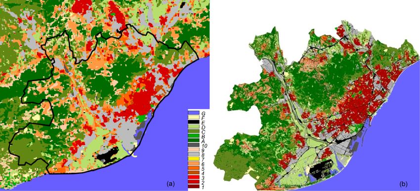
376                                                       J. Gilabert et al.: Assessing heat exposure to extreme temperatures

extreme temperature causes increased heat-related mortality        2000; Tromeur et al., 2012; Nakamura and Llasat, 2017). In
(Smid et al., 2019; Ingole et al., 2020).                          this framework heat vulnerability is understood as a com-
   There are many factors that influence the spatial and tem-      bination of heat exposure (based on high temperatures) and
poral climate variability in urban areas, such as different ur-    sensitivity (Wolf and McGregor, 2013; Bao et al., 2015; Inos-
ban morphologies and the thermal properties of the materi-         troza et al., 2016), where the last is related to population char-
als used to build such areas (Geletič et al., 2016; Li et al.,    acteristics and coping capacities. Although there are some
2016). One of the main topics usually studied to charac-           publications that study risk on an urban scale for extreme
terise the urban climate is the extreme temperatures in cities     heat events (Xu et al., 2012; Weber et al., 2015; Krstic et al.,
due to the UHI effect, which was first discussed back in the       2017; Eum et al., 2018), few have been studied from an LCZ
1940s (Balchin and Pye, 1947). Historically, a considerable        perspective. This paper therefore aims to assess heat expo-
body of research has been published on the phenomenon              sure using the LCZ classification in a coastal Mediterranean
(i.e. Oke, 1982; Lo et al., 1997; Arnfield, 2003; Voogt and        metropolitan region. Barcelona constitutes a good example
Oke, 2003; Chen et al., 2006; Mirzaei and Haghighat, 2010;         of a Mediterranean coastal megacity (port cities with a pop-
Giannaros et al., 2014; Lehoczky et al., 2017; Sobrino and         ulation greater than 1 million in 2005) (Hanson et al., 2011)
Irakulis, 2020). However, certain methodological inconsis-         that can be severely affected by climate change impacts. In
tencies have been revealed when comparing different ur-            effect, the annual mean temperature increase in the Mediter-
ban climate studies. One of the main reasons is the lack           ranean Basin is higher than the world average (1.5 ◦ C above
of standardisation to compare the properties that affect spe-      1880–1899 levels in 2018) and could be above 2.2 ◦ C in 2040
cific urban thermal behaviour (Stewart, 2011). Moving for-         without additional mitigation (Lionello et al., 2014; Cramer
ward from this premise, a new methodology based on the             et al., 2018; MedECC, 2019). Direct impacts on health pro-
urban climate zones defined by Oke (2004) and called the           duced by the frequency and intensity increase in heat waves
Local Climate Zone (LCZ) classification has emerged (Stew-         and tropical nights will be amplified by the urban-heat-island
art and Oke, 2012). LCZ classification establishes a system        effect, which is particularly important in Barcelona (Bac-
of standardisation for urban and rural areas and their ther-       cini et al., 2011; Martin-Vide and Moreno, 2020). Associated
mal responses. It proposes a classification with a total of 17     with this temperature increase, by 2050, for the lower-sea-
measurable categories based on a combination of geomet-            level-rise scenarios and current adaptation measures, cities in
ric, thermal, radiative and metabolic parameters that charac-      the Mediterranean will account for half of the 20 global cities
terise urban and peri-urban areas. By using this classification,   with the highest increase in average annual damage (Halle-
it is possible to study the effects of urban climate in more       gate et al., 2013).
spatial and temporal detail (Bechtel et al., 2015). Combina-          This study is a starting point for new research lines with
tions of built environment (Benzie et al., 2011; Inostroza et      three objectives in mind: (a) making changes to urban land
al., 2016) are well encompassed by the LCZ approach, and,          cover and observing the changes in heat exposure to high
along with socio-demographic factors (Nayak et al., 2018),         temperatures without having to resort to climate modelling,
this allows us to develop a geospatial distribution of heat ex-    (b) downscaling the temperature outputs of urban models to
posure (Dickson et al., 2012; Drobinski et al., 2014). Along       resolutions of under 100 m using the LCZ maps, and (c) ap-
the same line of research, the international project called        plying this methodology to climate change scenarios.
World Urban Database and Access Portal Tools (WUDAPT)
has created a portal with guidelines based on Earth observa-
tion data, with the aim of building a worldwide database of        2     Data and methods
cities, using the LCZ classification. This standardisation will
allow comparisons between cities while providing better data       2.1    Study area
for meteorological and climate models (Brousse et al., 2016;
Ching et al., 2018). Currently, the available, validated layer     The Metropolitan Area of Barcelona (AMB) and its sur-
for Barcelona on the WUDAPT portal is the one made in our          roundings have been selected for the application of the LCZ
studio to fill in the Metropolitan Area of Barcelona (AMB),        classification. AMB involves the city of Barcelona and 35 ad-
as explained in more detail in Sect. 3.1.                          joining municipal areas (Fig. 1). The AMB is situated in the
   Due to LCZ classification being originally designed to          northwest of the Mediterranean Basin and covers an area of
mainly describe the thermal characteristics of the different       636 km2 with a population of around 3.2 million. The city of
land covers and land uses, it is useful to apply it to esti-       Barcelona (∼ 1.6 million) is in its centre, between the rivers
mate the level of heat exposure (Vicedo-Cabrera et al., 2014;      Llobregat (south) and Besòs (north), the Catalan Coastal
Lowe et al., 2015; Achebak et al., 2019) to adverse climate        Range (west), and the Mediterranean Sea (east) (Fig. 1b).
conditions that is one of the main goals of this paper. There         The Barcelona municipality has been selected to anal-
are a wide range of definitions for the term “vulnerability”       yse the effect of high temperatures and apply the proposed
(UNISDR, 2009; Cutter, 1996; Llasat et al., 2009), which           methodology approach on a neighbourhood scale. Barcelona
depend on different physical and social factors (Cutter et al.,    is divided into 10 districts, which are subdivided into 73

Nat. Hazards Earth Syst. Sci., 21, 375–391, 2021                                    https://doi.org/10.5194/nhess-21-375-2021
J. Gilabert et al.: Assessing heat exposure to extreme temperatures                                                                 377

Figure 1. (a) Location of the Metropolitan Area of Barcelona (AMB), (b) Domain used to run the UrbClim model. The blue line marks the
border of the AMB, while the black line shows the municipality of Barcelona. The numbers indicate the weather stations used to assess the
LCZ–T relationship.

neighbourhoods. It covers an area of 101 km2 and has a pop-               Each one of these steps will be explained in detail in the
ulation density of over 15 000 inh./km2 , which is higher than         following sections in order to simplify the understanding of
New York City, Tokyo or New Delhi. In terms of climate,                this methodology in which each part is based on the results
Barcelona and its surroundings are characterised by hot sum-           of the previous one. The overall methodology followed con-
mers (25–27 ◦ C average temperature), and the thermal stress           stitutes a result of this work.
of high temperatures is accentuated by the proximity of the
sea, which results in a humid atmosphere. Total precipita-             2.3     LCZ mapping
tion in Barcelona is around 600 mm per year. Autumn is the
wettest season and has a highly irregular distribution of pre-         2.3.1    Data from official thematic cartography, satellite
cipitation, in many cases causing episodes of urban flooding                    images and weather stations
(Gilabert and Llasat, 2017; Cortès et al., 2018).
                                                                       In order to create the LCZ cartography, data shown in Ta-
2.2   Methodology design                                               ble 1 have been used. The LCZs were represented following
                                                                       two methods, as explained in Sect. 3. The land cover–land
In order to carry out this study, we followed the workflow             use method was based on using all the layers presented in Ta-
shown below:                                                           ble 1, except for the Landsat 8 image, which was only used
                                                                       with the WUDAPT methodology and the orthophoto to make
  1. LCZ mapping. A geographic information system                      the training areas.
     methodology based on land cover and land use (LCLU)
     maps has been applied to the entire AMB to improve the            2.3.2    Land cover and land use method and WUDAPT
     precision of the international WUDAPT method. The                          method
     WUDAPT method has also been applied to all the area
     shown in Fig. 1b, both inside and outside AMB, that               There are several proposals for mapping LCZs, whether with
     will be used as input of the climate model.                       a bottom-up or top-down approach (Brousse et al., 2016;
                                                                       Lelovics et al., 2014; Wang et al., 2017; Mitraka et al., 2015).
  2. Climate characterisation. The climate of the median-
                                                                       Each LCZ is defined by 10 variables (geometric, radiative
     and extreme-temperature distribution in Barcelona was
                                                                       and metabolic), which were tested and standardised by Stew-
     characterised from the outputs of the UrbClim model.
                                                                       art and Oke (2012) and are applied in this study.
  3. Heat exposure thresholds. Heat exposure thresh-                      Our study features an LCZ map that combines two differ-
     olds were defined based on the epidemiological                    ent mapping techniques (Fig. 2). For the administrative re-
     temperature–mortality model proposed by Achebak et                gion of the AMB (with a more extensive and detailed source
     al. (2018).                                                       of data), a methodology based on land cover and land use
                                                                       (LCLU) data was used that departs from the reclassification
  4. Thermal characterisation. A methodology was devel-                of the land use key for the existing high-resolution maps. The
     oped for the thermal characterisation of the LCZs and             LCLU data were combined with lidar data, which allowed us
     its assessment.                                                   to define the height of the buildings. There are other tech-

https://doi.org/10.5194/nhess-21-375-2021                                        Nat. Hazards Earth Syst. Sci., 21, 375–391, 2021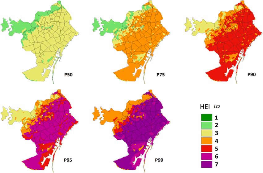
378 J. Gilabert et al.: Assessing heat exposure to extreme temperatures
Table 1. Vector and raster cartographic data and satellite images used to map the LCZ LCLU and LCZ WUDAPT methods.
Layer Information Spatial resolution Year Format
Urban Atlas 20 categories of urban fabric 5m 2012 Vector cartography
LCLU-Cat 241 categories 0.25 m 2009 Vector cartography
Building heights Height (m) (lidar) 0.5 m 2014 Vector cartography
Orthophoto Mosaic of aerial photos 0.25 m 2016 Raster cartography
Population Population by ages 62.5, 125, 250 m 2016 Vector cartography
Landsat 8 5 May 2015 30 m 2015 Raster satellite
niques that use similar methodologies to show LCZs, like in the coastal mountain range. The next most common class
those by Geletič and Lehnert (2016) or Skarbit et al. (2017). is LCZ C, which corresponds to scrubland and bush. Dealing
For the area outside the AMB, the international WUDAPT with land classified as urban, the most common types include
methodology was used, based on satellite Earth observation industrial estates (LCZ 8); areas with dense buildings less
data (Bechtel et al., 2015). This study improved accuracy than 25 m tall (LCZ 2); and category LCZ 6, which consists
through a population map and high-resolution orthophotos of open arrangements of mid-rise buildings. The WUDAPT
provided by the Cartographic and Geological Institute of Cat- map suffers from a lack of characterisation of urban areas,
alonia (ICGC). Both methodologies are summarised below. which is not the case for the LCLU map.
The LCLU method is based on different land cover and The resulting LCZ map is a high-resolution thematic vec-
land use maps (see Table 1), such as the Land Cover Map of tor base map (Fig. 2b), in which each polygon that makes up
Catalonia (LCLU-Cat), which uses both an extensive classi- the urban fabric is attributed to an LCZ category (Gilabert et
fication of up to 241 categories made by the Centre for Re- al., 2016). Finally, it was rasterised at a resolution of 100 m,
search on Ecology and Forestry Applications and the Urban applying an all shape filter, so that it could be used as an input
Atlas (UA). The first thematic map was used to define the for the UrbClim model. The method we followed is shown
land cover types and density of vegetation. The UA distin- in the workflow diagram (Fig. 4). There are similar exam-
guishes 20 categories of urban areas and discerns between ples in the literature, such as the LCZ map for Île-de-France
urban fabric type and density, which is why it is very useful (http://www.institutparisregion.fr, last access: 23 July 2020)
for the first 10 categories of LCZ classification. Each LCLU or the LCZ LCLU map of Vienna (Hammerberg et al., 2018).
category corresponds to one of the descriptions of the differ- The WUDAPT method (Bechetel et al., 2015) allows us to
ent morphological parameters that define the LCZs. Building create a 100 m × 100 m raster map based on Earth observa-
heights is another layer of the map and was made with a lidar tion data from remote sensing. The representative regions of
sensor, which was also used to discern between the different interest are chosen for proposed LCZ categories from Earth
building types of each LCZ. observation satellite data, with the use of very high resolu-
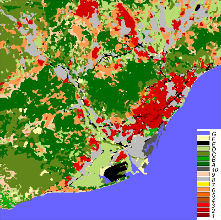
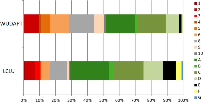
Figure 3 shows the difference between the total coverage tion aerial orthophotos as the ground truth. The LCZ map,
of each LCZ when obtained from the LCLU and from WU- made by the first author of this paper using the WUDAPT
DAPT maps in AMB (Fig. 2). In the WUDAPT approach, proposal, is officially presented on the project portal and is
52.8 % of the surface area of the AMB consists of urban ar- available for download (http://www.wudapt.org, last access:
eas (LCZs 1–10 and E), while in the high-resolution map 23 July 2020). This method has been applied to an extended
(LCLU approach), the same type of coverage occupies just area as is shown in Fig. 5.
37.3 %. It is a consequence of the difference in the LCZ char- A multi-resolution grid shape file (62.5, 125 and 250 m)
acterisation processes that both methods follow. Although 17 containing information on the population as registered in
LCZs are distinguished in the two methods, WUDAPT uses 2016 made by the Statistical Institute of Catalonia (Gener-
the spectral radiance provided by satellite images and applies alitat de Catalunya and Institut d’Estadística de Catalunya,
a supervised classification based on a random-forest general- 2015) was used to correct the peri-urban areas of AMB where
isation method based on training zones (Bechtel et al., 2015). rural activities cannot be well identified. The orthophoto was
On the contrary, the method of LCLU proposed here analy- used to check and correct any categories and the limits be-
ses the intrinsic variables that characterises each category of tween them.
LCZ classification, and consequently it has major integrity Figure 5 shows the resulting map combining the LCLU
and quality. That is to say, it has a better resolution. In both method (in raster format) for the administrative region of the
methods, we can see that the natural-forest category (LCZ A) AMB and the WUDAPT method for the rest of the study area
is the most common, accounting for 24.1 % and 18.4 % of the with a final resolution of 100 m.
land respectively. This is due to the fact that the Metropolitan
Area of Barcelona includes Serra de Collserola Natural Park
Nat. Hazards Earth Syst. Sci., 21, 375–391, 2021 https://doi.org/10.5194/nhess-21-375-2021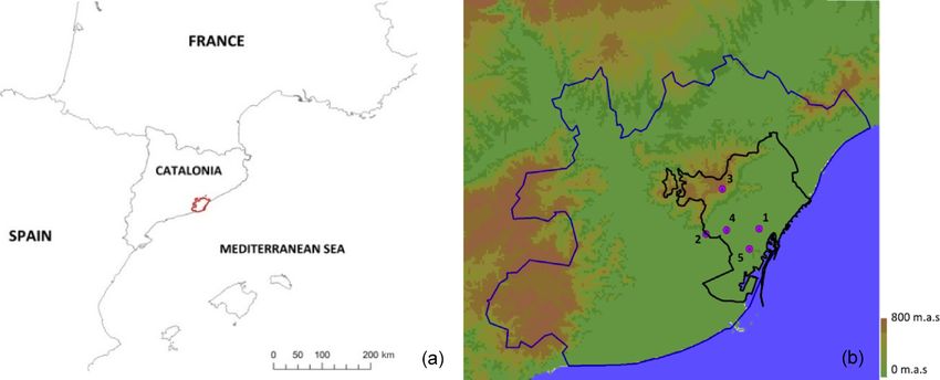
J. Gilabert et al.: Assessing heat exposure to extreme temperatures                                                       379

Figure 2. LCZ maps: (a) WUDAPT method, (b) LCLU method.

                                                                 of the Pan-European Urban Climate Service (PUCS) project
                                                                 (H2020, 2017–2019), the urban climate of Barcelona has
                                                                 been modelled until 2100, keeping in mind different repre-
                                                                 sentative concentration pathways (RCPs) to observe the con-
                                                                 sequences of climate change on an urban scale. Barcelona
                                                                 was chosen, among other European cities, and VITO and IS-
                                                                 Global were the organisations responsible for modelling this
                                                                 city.
                                                                    UrbClim model uses a land surface and a soil–vegetation–
                                                                 atmosphere transfer scheme that is designed to deal with ur-
                                                                 ban surfaces. Each surface grid cell in the model is made up
Figure 3. Percentage of the area covered by each LCZ using WU-   of portions of vegetation, bare soil and urban surface cover,
DAPT and LCLU inside AMB.                                        which are all represented using LCZ mapping. A set of trans-
                                                                 fer equations, together with appropriate parameter values for
                                                                 albedo, emissivity, and aerodynamic and thermal roughness
2.4   Weather stations                                           length, is used to simulate the heat transfer in each surface
                                                                 grid cell. The large-scale atmospheric conditions are used
Table 2 shows the weather stations within the municipality of    as lateral and upper boundary conditions. The 3D bound-
Barcelona that have been used to evaluate and compare the        ary layer model represents a simplified atmosphere by using
characterisation of the LCZ with the daily average tempera-      the continuity equations for horizontal momentum, potential
ture outputs of the UrbClim model. LCZ and height informa-       temperature, specific humidity and mass.
tion are also attached.                                             The simulations for the 1987–2016 period were used for
                                                                 this period. The UrbClim simulations cover a large domain
2.5   UrbClim model simulation                                   containing 401 × 401 horizontal grid points at a 100 m res-
                                                                 olution (40 × 40 km approximately) and 19 vertical levels
UrbClim is an urban boundary layer climate model specifi-        within the lower 3 km of the troposphere. It covers the en-
cally designed to simulate temperature at a very high spatial    tire geographical area of the Metropolitan Area of Barcelona,
resolution (here at 100 m; De Ridder et al., 2015). The model    including the neighbouring highly populated cities. The driv-
consists of a land surface scheme with simplified urban          ing model data are updated every 3 h using ERA-Interim re-
physics coupled to a 3D atmospheric boundary layer. Urb-         analysis (Dee et al., 2011), which runs at a spatial resolu-
Clim is faster than high-resolution mesoscale climate models     tion of T255 (approximately 70–80 km). The UrbClim model
by at least 2 orders of magnitude (García-Díez et al., 2016),    directly downscales the ERA-Interim reanalysis data to a
making the very long runs that are necessary for climate-        100 m resolution. The climate distributions of the daily mean
change-related studies possible. UrbClim has been recently       temperature (Tmean ), maximum temperature and dew point
validated in several European cities, including Barcelona        temperatures were calculated for all the summer months
(García-Díez et al., 2016). Currently, within the framework      (JJA). The maximum temperature provides an estimate of

https://doi.org/10.5194/nhess-21-375-2021                                 Nat. Hazards Earth Syst. Sci., 21, 375–391, 2021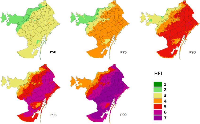
380                                                        J. Gilabert et al.: Assessing heat exposure to extreme temperatures

Figure 4. Workflow used to obtain the LCZ LCLU model.

Table 2. Weather stations in Barcelona used to assess the LCZ–T relationship based on daily mean temperatures.

                           ID    Weather stations      Series        Years    LCZ    Z (m a.s.l.)   Variable
                           1     Raval                 1997–2016        19    2               33    T   daily
                           2     Zona Universitària    1997–2016        19    C               79    T   daily
                           3     Fabra                 1987–2016        29    A              411    T   daily
                           4     Can Bruixa            1987–2015        28    2               61    T   daily
                           5     Montjuïc              2004–2015        11    B               90    T   daily

                                                                      the worst conditions that can be expected. This is important
                                                                      for risk management and avoiding heatstroke, which usually
                                                                      occurs during the hours of the day when the temperature
                                                                      reaches its highest value. The dew point temperature (Tdew )
                                                                      was used as a starting point to calculate the humidex (humid-
                                                                      ity index; Eq. 1), which describes the perceived thermal feel-
                                                                      ing of a person, by combining the effect of heat and humidity
                                                                      (Masterton and Richardson, 1979). Barcelona has quite high
                                                                      relative humidity during the summer months, which means
                                                                      that the humidex increases considerably.

                                                                                                                    1            1
                                                                                                        5417.7530 273.16 + 273.15+T
                                                                      Humidex = Tmean + 0.5555[6.11e                                  dew

                                                                              − 10]                                                             (1)

                                                                      2.6    Quantifying heat exposure by temperature

                                                                      The next step consists of reclassifying the maps of the pro-
                                                                      posed distributions for the daily mean temperature, keep-
                                                                      ing in mind the impact that they can have on health. This
                                                                      was carried out using the results provided in the study by
                                                                      Achebak et al. (2018), in which a distributed-lag nonlinear
                                                                      model was used to model the short-term delayed relation
Figure 5. LCZs used in the UrbClim model based on workflow
shown in Fig. 4.
                                                                      between daily summer temperature and mortality data from
                                                                      cardio-respiratory diseases in Barcelona (and 46 other cities),
                                                                      over a similar period of time modelled (Fig. 6). This makes it
                                                                      possible to objectively establish the thresholds for health rel-

Nat. Hazards Earth Syst. Sci., 21, 375–391, 2021                                        https://doi.org/10.5194/nhess-21-375-2021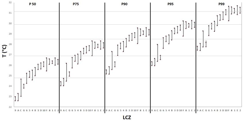
J. Gilabert et al.: Assessing heat exposure to extreme temperatures 381
3 Results
3.1 UrbClim temperature outputs and HEI maps
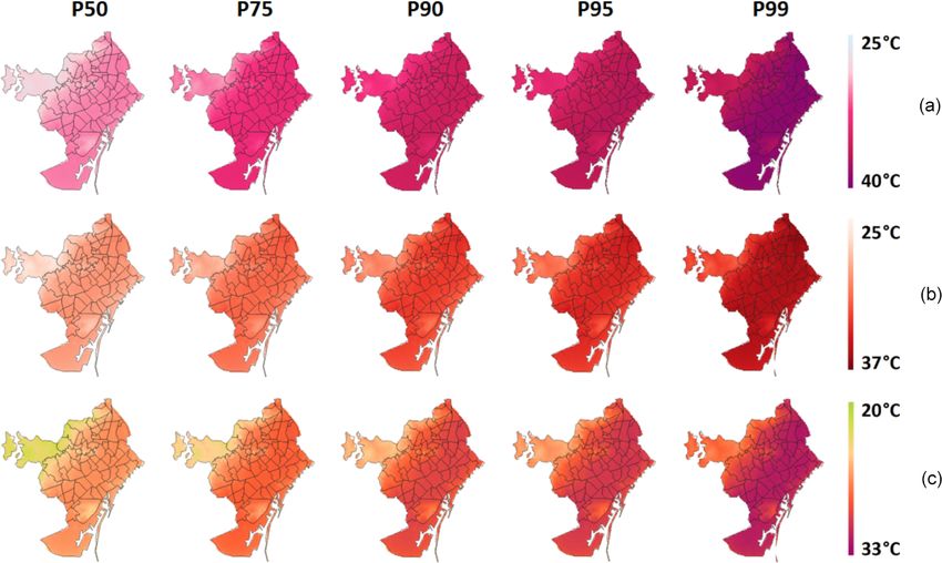
In order to analyse the impact of the different LCZs in the
distribution of high temperatures in summer, the maps of
maximum and daily mean temperature corresponding to per-
centiles P50, P75, P90, P95 and P99 have been built (Fig. 7).
Barcelona has a high relative humidity due to proximity to
the sea that increases warm perception, and, for this reason,
the cartography of the average daily humidex value has also
been represented.
As we can see in Fig. 7, there is a very similar spatial dis-
tribution pattern. The lowest temperatures are in the most
remote area of the coast, and they are mainly associated
Figure 6. Relative risk (RR) curve based on mortality due to sum-
with categories LCZ A and LCZ 9 (mainly covering areas
mer daily temperature (JJA) in Barcelona for the 1980–2015 period of woodland or very low density buildings). A cooling ef-
(Achebak et al., 2018). fect can also be noted in the most important parks in the
city, as well as on the seafront, because of the sea breeze
Table 3. Temperature thresholds associated with heat exposure (the UrbClim model underestimates the sea breeze effect in
caused by high temperatures in reference to Fig. 5. A heat expo- Barcelona; García-Diez et al., 2016). The highest tempera-
sure index (HEI) is assigned to each temperature range. tures can be found in the centre of the city, with a tendency
to increase in a north-easterly direction.
RR HEI ◦C We saw that P99 of the humidex reached 39 ◦ C. In
Barcelona, without taking humidity into account, the aver-
1.0 1 18–20
age temperature in the city can reach above 30 ◦ C. Even so,
1.2 2 20–24.7
normal temperatures during the summer are around 27 ◦ C. In
1.4 3 24.7–26.9
1.6 4 26.9–28.5 Mediterranean cities, relative humidity is important since it
1.8 5 28.5–29.8 is usually high, a fact that affects temperature (Diffenbaugh
2.0 6 29.8–31.1 et al., 2007). In this sense, we observe that the humidex can
> 2.0 7 > 31.1 register temperatures on the order of 5 ◦ C higher than the sen-
sible temperature. This study has focused on sensible temper-
ature because the curve that defines the heat exposure index
ative risks (RRs), based on temperature. For instance, an RR has been made for sensible temperature. In any case, we must
value of 1.20 means that the relative risk of mortality is 20 % bear in mind that the temperature or heat stress may be higher
higher at a given level of temperature exposure compared to due to the greater humidex.
a baseline optimum temperature (e.g. temperature of mini- Figure 8 shows maps of HEI distribution reclassified with
mum mortality, when RR = 1). Relative risks are statistically the UrbClim output of daily mean temperature according to
significant when the lower bound of the confidence interval the proposed thresholds shown in Sect. 2.6. This reclassifica-
is greater than 1. tion turns the extreme-temperature maps or hazard maps into
We are assuming that the curve is applicable to all districts heat exposure maps. It can be seen that the HEI is lower in
of the city (Achebak et al., 2018). Table 3 has been built for areas with higher altitude and in inter-urban parks (such as
RR intervals of 0.2 (20 %) following Fig. 6. Each RR interval the Montjuïc park located in the SE of the map); although
has been associated with a heat exposure index (HEI) that in- when P90 is surpassed, the HEI value goes over level 5 for
cludes temperature intervals based on the curve of Achebak most of the urban fabric. Note that P50 shows an increase in
et al. (2018). Barcelona deals with an HEI value of 1 for tem- the relative risk of mortality of 40 %.
peratures between 18 and 20 ◦ C up to an HEI value of 7 for
temperatures above 31.1 ◦ C which would mean a very high 3.2 Thermal characterisation of the LCZs
relative risk of mortality associated with high temperatures.
The use of seven HEI categories has the advantage that it can In this section we aim to match up each LCZ with a deter-
be applied to any city by adjusting them to the temperature mined thermal behaviour to create a methodology that will
values of that city and to the RR curve considered. allow us to estimate the heat exposure to high temperatures
from these data.
First, for each climatic percentile (P50, P75, P90, P95 and
P99) of daily mean temperature (although it could also be
https://doi.org/10.5194/nhess-21-375-2021 Nat. Hazards Earth Syst. Sci., 21, 375–391, 2021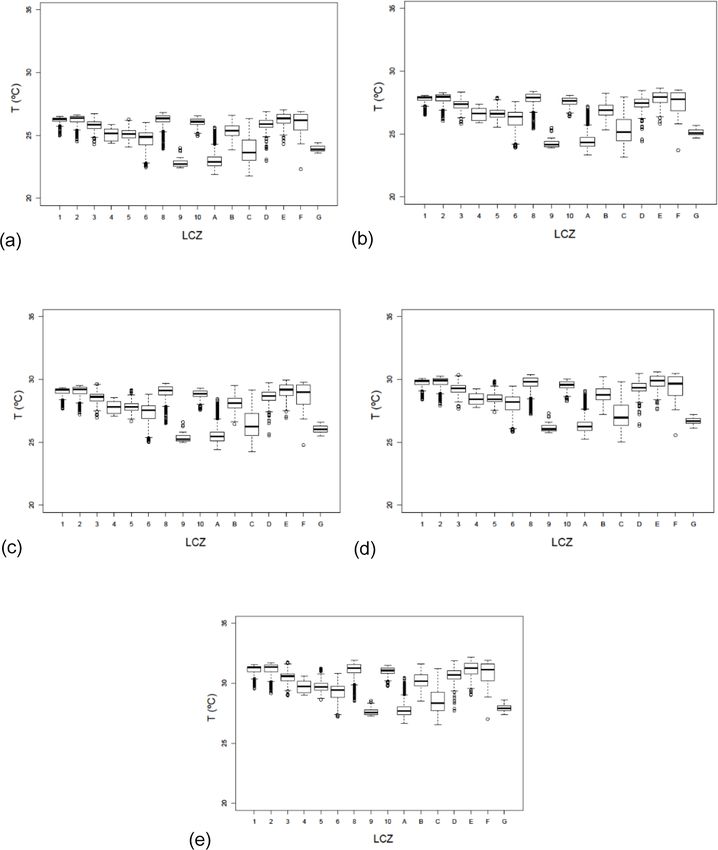
382                                                         J. Gilabert et al.: Assessing heat exposure to extreme temperatures

Figure 7. Climatological conditions in summer modelled by UrbClim (1987–2016): (a) humidex, (b) daily maximum temperature and
(c) daily mean temperature, for the different distributions (P50, P75, P90, P95 and P99).

Figure 8. Maps of HEI for the different probability distributions proposed (P50, P75, P90, P95 and P99).

performed for the maximum temperature and humidex) we                     In order to characterise each LCZ, we tested its normal-
analysed the thermal response of the LCZ (LCZ–T ) (Fig. 7).            ity and the differentiated behaviour of each probability den-
To do so we compared, pixel by pixel, the temperature maps             sity curve adjusted to each LCZ. The results of the normal-
with the LCZ maps, and we built a box plot for each LCZ                ity tests (based on the central limit theorem) and compara-
(Fig. 9).                                                              ble variations on the relation between LCZ–T indicated that

Nat. Hazards Earth Syst. Sci., 21, 375–391, 2021                                         https://doi.org/10.5194/nhess-21-375-2021
J. Gilabert et al.: Assessing heat exposure to extreme temperatures                                                                       383

Figure 9. Box plots for the thermal characterisation of the LCZ for different distributions: (a) P50, (b) P75, (c) P90, (d) P95 and (e) P99.

https://doi.org/10.5194/nhess-21-375-2021                                           Nat. Hazards Earth Syst. Sci., 21, 375–391, 2021
384                                                        J. Gilabert et al.: Assessing heat exposure to extreme temperatures

ANOVA may be used for testing whether the differences in            Table 4. Standard deviations for the LCZs for the different per-
LCZ mean temperatures outlined above are significant or not         centiles of temperature.
(Geletic et al., 2016). LCZs C, F and 6 do not follow a normal
distribution (at 95 %) although they tend towards it. This is               LCZ      P50      P75     P90      P95     P99
due to the high thermal variability in these categories. There              1       0.301   0.325    0.349   0.363    0.419
were statistically significant differences in mean land surface             2       0.356   0.379    0.396   0.401    0.475
temperatures between most LCZs, but LCZs 4 and 5 were                       3       0.450   0.468    0.486   0.489    0.552
recognised as zones that were less distinguishable from other               4       0.528   0.530    0.535   0.522    0.569
LCZs. Once we had the temperature distribution it was pos-                  5       0.467   0.488    0.504   0.500    0.541
sible to map the HEI.                                                       6       0.821   0.841    0.872   0.843    0.804
   Transposing the model onto LCZ maps allowed us to map                    8       0.465   0.499    0.527   0.531    0.580
heat exposure distributions for Barcelona. This methodology                 9       0.456   0.474    0.461   0.441    0.379
has the advantage that it can be transferred to other cities                10      0.319   0.338    0.339   0.338    0.322
                                                                            A       0.686   0.712    0.725   0.705    0.649
because it relates each LCZ with an HEI value. It is only
                                                                            B       0.554   0.580    0.603   0.616    0.641
necessary to have the LCZ map and know some temperature                     C       1.090   1.128    1.168   1.128    1.088
values in the city to calibrate the model. In the case that there           D       0.550   0.572    0.596   0.586    0.612
is not an RR–T curve available, the same HEI as in this paper               E       0.530   0.561    0.599   0.595    0.678
could be applied.                                                           F       0.848   0.918    0.960   0.955    0.978
   Figure 9 shows that LCZs 8 (large low-rise buildings), 1                 G       0.224   0.265    0.297   0.294    0.289
(compact high-rise), E (asphalt) and 2 (compact mid-rise)
(from highest to lowest) usually have the highest tempera-
tures. These LCZs in general terms correspond to the cate-          lows for performing a simulation of the impact on tempera-
gories with high admittance and high permeability (Stewart          ture distribution of potential modifications to the urban mor-
and Oke, 2012). In contrast, the lowest temperatures corre-         phology.
spond to LCZs 9 (sparsely built), A (dense trees), C (bushes)          As explained in the methodology, seven ranges of temper-
and G (water), which are wooded areas and parks on the out-         ature have been defined according to different relative risk
skirts of the city. On the other hand, crops and bare land          thresholds (Table 3) established by the curve proposed in the
(LCZs C and F) show very variable behaviour, as during the          study by Achebak et al. (2018) (Fig. 6). By characterising
day they tend to be surfaces that store and retain heat, while      the LCZs from the model represented in Fig. 11, the maps
during the night their behaviour registers temperatures below       of the heat exposure index associated with high temperatures
the average of the sample. These surfaces are characterised         for different probabilistic scenarios have been built. The sce-
by a large temperature range given the marked contrast be-          nario corresponding to P75 of the temperature would imply
tween day and night.                                                a ratio of relative risk of mortality increase of 60 %, and this
   Table 4 shows that the more extreme the percentile, the          would be 80 % in a scenario according to P90.
larger the standard deviation, as expected. Besides this, the
more marked deviations correspond to LCZs C and F, which            3.4   Assessment and comparison of the LCZ–T
correspond to wooded or bare areas and which show less                    relationship
thermal inertia. On the other hand, category C is very highly
influenced (in the case of Barcelona) by orientation, as there      The results of the LCZ–T relationship as well as the results
are zones located in shaded parts of valleys while other zones      of the urban climate model (UC) have been compared with
are in the sunny ones, which has a direct impact on the de-         the distribution of temperature obtained from series of over
viation. In the case of category C, we observed that it corre-      10 years for five weather stations (Table 2) located in differ-
sponds to land use that is not very representative in spatial       ent LCZs in the municipality of Barcelona. Root mean square
terms.                                                              errors (RMSEs), the differences between the output of both
                                                                    sets of results (UrbClim model and LCZ–T relationship) and
3.3   Mapping the heat exposure with LCZs                           observations have been obtained in order to compare the re-
                                                                    sults (Tables 5 and 6). We want to highlight that UrbClim
Figure 10 shows the average behaviour of the LCZs for dif-          has already been validated in Barcelona by García-Díez et
ferent temperature percentiles (P50, P75, P90, P95, P99).           al. (2016) as outlined in Sect. 2.6. Table 5 shows that differ-
The values corresponding to the range between the 25th and          ences in absolute value are lower than 1.2 ◦ C. In all the cases
75th percentiles of each LCZ for each probability scenario          they are equal to or below 0.5 ◦ C for the percentile of 50, and
have been adjusted to a logarithmic curve that can be very          this is also the case for the percentile of 75 with the excep-
useful for building heat exposure maps for high temperatures        tion of the Raval station, which is placed in the oldest part
based on the thermal properties of the LCZ. Knowing the             of the city. It should also be kept in mind that a stand-alone
temperature distribution for each category and scenario al-         observation is not the same as an aerial 100×100 m observa-

Nat. Hazards Earth Syst. Sci., 21, 375–391, 2021                                     https://doi.org/10.5194/nhess-21-375-2021
J. Gilabert et al.: Assessing heat exposure to extreme temperatures 385 Figure 10. Characterisation of every LCZ with the daily mean temperature (1987–2016) for each probability scenario. Each bar shows P25 and P75, around the median for each LCZ (ordered from lowest to highest temperature). The horizontal grey lines are the different HEI scenarios (2 to 7, low to high). Figure 11. Cartography of the heat exposure index (HEI) in reference to thermal characterisation of Barcelona by LCZs for different per- centiles (LCZ–T ) as shown in Table 3. https://doi.org/10.5194/nhess-21-375-2021 Nat. Hazards Earth Syst. Sci., 21, 375–391, 2021
386                                                       J. Gilabert et al.: Assessing heat exposure to extreme temperatures

tion, and this fact is particularly important when the weather     metal structures). The urban LCZ with the lowest tempera-
station is surrounded by buildings.                                tures is 9, which is almost non-existent in Barcelona and is
   The HEI maps drawn up using the LCZs were compared              located mainly in zones in the Catalan Coastal Range with
with the map based on temperature distribution created by          a significant altitudinal slope. Another urban LCZ with low
UrbClim (Table 6). Coincidences between pixels for both            relative temperatures commonly found in the city is 6, which
models are above 80 % for percentiles P50, P75 and P90, and        is mainly located in the neighbourhoods furthest away from
they are more than 60 % in all cases.                              the coast and closer to the mountain. These neighbourhoods
                                                                   have a higher percentage of urban green cover, less dense
                                                                   buildings and some of the highest gross domestic products
4   Discussion and conclusions                                     per capita in the city.
                                                                      The paper has also introduced the heat exposure index
This paper presents a methodology to characterise the dis-         (HEI), which evaluates the increase in the risk of mortality
tribution of daily mean temperature in reference to the Lo-        ratio as a consequence of heat exposure in reference to the
cal Climate Zone (LCZ) mapping in different temperature            model proposed by Achebak et al. (2018) which connects
scenarios in summer (June–July–August). The climate per-           relative risk of mortality caused by cardio-respiratory fail-
centiles have been obtained for the period 1987–2016 and           ure with the effects of high temperatures. This index, asso-
applied at a 100 m resolution to the city of Barcelona. Al-        ciated with each LCZ once the temperature has been associ-
though other authors have already worked with the relation-        ated with it, allows for the mapping of the HEI. The com-
ship between thermal behaviour and LCZ category (Stew-             parison between the heat exposure index maps elaborated
art et al., 2014; Skarbit et al., 2015; Geletič et al., 2016;     directly from the temperature outputs produced by the Ur-
Verdonck et al., 2018), they have usually applied land sur-        bClim model and those produced from LCZ cartography is
face temperature satellite images for the summer months and        well suited to simulating heat exposure index maps for sce-
short time periods. Other characterisations of LCZ classifi-       narios corresponding to percentiles of temperature between
cation using weather stations can also be found in Alexan-         50 % and 90 %, and, in the case in which there is no coin-
der and Mills (2014) and Kotharjar and Bagade (2018). In           cidence between the HEI value in the pixel, it is more usual
these cases, these authors have worked with climate series         to have underestimation than overestimation. In the case of
from observational data. The advantage of the methodology          Barcelona, the distribution of temperatures for P90 (about 3–
proposed here, in which the LCZ distribution has been com-         4 ◦ C compared to average conditions) leads to an increase in
pared with the outputs of a high-resolution climate model          the relative risk of mortality of 80 %, and the increase is 40 %
(UrbClim), is that the relationship has been established from      in the case of P50.
long-term climate series and for the entire selected region.          This paper also provides comparison of two methodolo-
Currently, there are multiple studies characterising LCZs us-      gies to map LCZs: WUDAPT and the land cover–land use
ing urban model outputs (Aminipouri et al., 2019; Beck et          (LCLU) method based on land use maps. The international
al., 2018; Geletič et al., 2018; Kwok et al., 2019; Unger et      standard method WUDAPT is exclusively based on satel-
al., 2018), but there are not many studies with climatic ouputs    lite Earth observation data (Ching et al., 2018). LCLU is
that span as many years.                                           based on land use maps, the Urban Atlas, lidar measurements
   The results of this methodology applied to the Metropoli-       and orthophotos. LCLU has been applied to the Metropoli-
tan Area of Barcelona have shown a major difference be-            tan Area of Barcelona, and WUDAPT has been applied to
tween the thermal response in summer for the different LCZs        the entire region (inside and outside) the AMB. The WU-
than that obtained from some satellite images. In terms of         DAPT map suffers from a lack of characterisation of differ-
land use, LCZs A and C, which belong to the most prevalent         ent types of urban areas, which is not the case for the land
categories, show the lowest temperatures, consistent with the      cover–land use method. Therefore, when the required data
majority of studies carried out (e.g. Geletič et al., 2016). In   are available, it is better to apply the LCLU methodology
our case, category C shows a wider interquartile range than        than the WUDAPT one. In this study, the curve of Achebak
the other types. This is because this category is found in dif-    et al. (2018) was taken into account as representative of the
ferent altitudes along the Catalan Coastal Range and in areas      whole of Barcelona city. In the future, it would be good to
with different orientations. Regarding category B, attributed      have a similar curve for different districts of the city. In ad-
to the majority of inter-urban parks, it shows temperatures        dition to this, future work could include mapping sensitivity,
below those of the most typical urban zones.                       taking into account coping capacities based on gross domes-
   The highest daily mean summer temperatures in Barcelona         tic product (GDP), or the social structure of the neighbour-
are concentrated in LCZs 2, E, 1, 8, F and 10, with LCZs 2, 1      hood. This would include vulnerability.
and E being the most representative of urban planning in the          In conclusion, the LCZ–T relation based on the character-
city centre. With regard to LCZs 8 and 10, these are zones         isation of the average temperature for each LCZ correspond-
that tend to record high temperatures due to the nature of         ing to different percentile distributions allows us to consider
the activities and materials on the land cover (in most cases,     adaptive methods, proposing changes to more sustainable ur-

Nat. Hazards Earth Syst. Sci., 21, 375–391, 2021                                    https://doi.org/10.5194/nhess-21-375-2021
J. Gilabert et al.: Assessing heat exposure to extreme temperatures 387
Table 5. Temperature for each distribution scenario (DIST) and weather station observed (OB), modelled by UrbClim (UC) and estimated
from the distribution of temperature (the mean value is taken) for each LCZ (LCZ–T ). The difference (1) between them is also shown. All
the values are expressed in degrees Celsius. ZU denotes Zona Universitària.
DIST OB UC LCZ–T 1OB − UC 1OB − LCZ–T
1 – Raval (LCZ 2) P50 25.6 26.1 26.1 0.5 0.5
P75 26.8 27.6 27.6 0.8 0.8
P90 27.8 28.9 28.9 1.1 1.1
P95 28.5 29.6 29.6 1.1 1.1
P99 30.2 31.1 30.9 0.9 0.7
2 – ZU (LCZ C) P50 24.5 24.7 24.6 0.2 0.1
P75 25.8 26.2 26.2 0.4 0.4
P90 26.6 27.3 27.3 0.7 0.7
P95 27.2 28.1 27.9 0.9 0.7
P99 28.5 29.5 29.2 1 0.7
3 – Fabra (LCZ A) P50 23.1 23.1 22.9 0 −0.2
P75 24.6 24.7 24.3 0.1 −0.3
P90 25.9 25.8 25.5 −0.1 −0.4
P95 26.5 26.6 26.2 0.1 −0.3
P99 27.3 27.5 27.7 0.2 0.4
4 – Can Bruixa (LCZ B) P50 25.2 26.1 25.4 0.9 0.2
P75 26.8 27.6 26.9 0.8 0.1
P90 27.9 28.9 28.1 1 0.2
P95 28.6 29.6 28.8 1 0.2
P99 30 30.9 30.2 0.9 0.2
5 – Montjuïc (LCZ B) P50 24.8 25.2 25.0 0.4 0.2
P75 26.3 26.8 26.5 0.5 0.2
P90 27.3 28 27.7 0.7 0.4
P95 27.8 28.6 28.4 0.8 0.6
P99 29.1 30.1 29.8 1 0.7
Table 6. Number of pixels where the HEI obtained through the associated heat exposure index. Another possibility is being
LCZ–T model (Fig. 11) underestimates, overestimates or coincides able to separate the heat exposure levels on an LCZ map with
with the HEI provided by the urban climate model (Fig. 6) for the higher spatial resolutions from those used in weather models
different scenarios. Percentage of coincidences and RMSE are also and climate models.
shown.
Model P50 P75 P90 P95 P99
Data availability. The satellite data to apply the WUDAPT
Underestimate 284 671 1711 2789 2289 methodology were obtained from the official USGS EarthExplorer
Good 9687 8762 8175 6316 6823 website: https://earthexplorer.usgs.gov/ (Geological Survey (U.S.)
Overestimate 247 785 332 1103 1106 and EROS Data Center, 1980). The Google Earth Pro and SAGA
% correct 95 86 80 62 67 open-source software were used to reproduce the WUDAPT work-
RMSE 0.23 0.38 0.45 0.62 0.58 flow proposal. The data to map the LCZs at a vector resolution are
public data – the Urban Atlas and the LCLU-Cat obtained from the
following URLs: https://www.creaf.uab.es/mcsc/ (CREAF, 2009)
and https://land.copernicus.eu/local/urban-atlas/urban-atlas-2012
ban planning, for example the use of green or white cover. (EEA, 2012) . Lidar data belong to the ICGC and must be requested.
The data were obtained in the framework of the Industrial Doctor-
The advantage of the proposed methodology is that it allows
ate programme (ref. 2015-DI-038). The orthophoto was obtained
us to obtain a heat exposure distribution for summer tempera- using the WMS link, https://www.icgc.cat/es/Administracion-
tures without having to resort to climate models, by applying y-empresa/Servicios/Servicios-en-linea-Geoservicios/WMS-
the model of temperature distribution associated with each y-teselas-Cartografia-de-referencia/WMS-Mapas-y-ortofotos-
LCZ. It can also be useful to perform different experiments vigentes (Institut Cartogràfic i Geològic de Catalunya, 2015),
modifying land use and land coverage applied to the car- and the population data were obtained from the public URL,
tography and, consequently, the LCZ distribution and their https://biblio.idescat.cat/publicacions/Record/21104 (Generalitat
https://doi.org/10.5194/nhess-21-375-2021 Nat. Hazards Earth Syst. Sci., 21, 375–391, 2021388 J. Gilabert et al.: Assessing heat exposure to extreme temperatures
de Catalunya and Institut d’Estadística de Catalunya, 2014). The Achebak, H., Devolder, D., and Ballester, J.: Trends in temperature-
meteorological data to validate the model were provided by the related age-specific and sex-specific mortality from cardiovas-
two official and public services in Catalonia: AEMET and SMC. cular diseases in Spain: a national time-series analysis, Lancet
The UrbClim model used public ERA-Interim reanalysis data from Planet. Health, 3, e297–e306, 2019.
https://apps.ecmwf.int/datasets/data/interim-full-daily/levtype=sfc/ Alexander, P. and Mills, G.: Local climate classification and
(Berrisford et al., 2009). The model was run at the VITO centre Dublin’s urban heat island, Atmosphere-Basel, 5, 755–774,
under the PUCS project (no. 730004)). The RR model was based 2014.
on the model presented in the article of Achebak et al. (2018). Aminipouri, M., Knudby, A. J., Krayenhoff, E. S., Zickfeld, K., and
Middel, A.: Modelling the impact of increased street tree cover
on mean radiant temperature across Vancouver’s local climate
Author contributions. JG conceived the study, designed and carried zones, Urban For. Urban Gree., 39, 9–17, 2019.
out the data analysis, and wrote the paper. MCL, JC and JB partic- Arnfield, A. J.: Two decades of urban climate research: a review of
ipated in defining the analysis and methodology and contributed to turbulence, exchanges of energy and water, and the urban heat
interpreting the results and to writing the paper. DL and AdL ran island, Int. J. Climatol., 23, 1–26, 2003.
the UrbClim model and prepared the output data. Baccini, M., Kosatsky, T., Analitis, A., Anderson, H. R., D’Ovidio,
M., Menne, B., Michelozzi, P., and Biggeri, A.: Impact of heat
on mortality in 15 European cities: attributable deaths under dif-
Competing interests. The authors declare that they have no conflict ferent weather scenarios, J. Epidemiol. Commun. H., 65, 64–70,
of interest. 2011.
Balchin, W. G. V. and Pye, N.: A micro-climatological investigation
of bath and the surrounding district, Q. J. Roy. Meteor. Soc., 73,
297–323, 1947.
Acknowledgements. Our thanks go to M-CostAdapt (TM2017-
Bao, J., Li, X., and Yu, C.: The construction and validation of the
83655-C2-2-R) research projects (MINECO/AEI/FEDER, UE),
heat vulnerability index, a review, Int. J. Env. Res. Pub. He., 12,
an ERC Consolidator Grant awarded to Gara Villalba (818002-
7220–7234, 2015.
URBAG), and the Water Research Institute (IdRA) at the University
Bechtel, B., Alexander, P. J., Böhner, J., Ching, J., Conrad, O., Fed-
of Barclona. The authors would like to thank the European Environ-
dema, J., Mills, G., See, L., and Stewart, I.: Mapping local cli-
ment Agency (EEA), Centre for Ecological Research and Forestry
mate zones for a worldwide database of the form and function of
Applications (CREAF) and Metropolitan Area of Barcelona for
cities, ISPRS Int. Geo.-Inf., 4, 199–219, 2015.
making the land use maps available. We would also like to thank
Beck, C., Straub, A., Breitner, S., Cyrys, J., Philipp, A., Rathmann,
the State Meteorological Agency (AEMET) and the Meteorological
J., Schneider, A., Wolf, K., and Jacobeit, J.: Air temperature char-
Service of Catalonia (SMC) for the weather station data. Finally, we
acteristics of local climate zones in the Augsburg urban area
want to thank Hicham Achebak for giving us the RR model.
(Bavaria, southern Germany) under varying synoptic conditions,
Joan Ballester gratefully acknowledges funding from the Euro-
Urban Clim., 25, 152–166, 2018.
pean Union’s Horizon 2020 research and innovation programme un-
Benzie, M., Burningham, K., and Hodgson, N.: Vulnerability to
der grant agreement nos. 865564 (European Research Council Con-
Heat Waves and Drought: Case Studies of Adaptation to Climate
solidator Grant EARLY-ADAPT), 727852 (project Blue-Action)
Change in South-West England, York, UK, The Joseph Rowntree
and 730004 (project PUCS) and from the Ministry of Science and
Foundation, 2011.
Innovation (MCIU) under grant agreement nos. RYC2018-025446-
Berrisford, P., Dee, D. P. K. F., Fielding, K., Fuentes, M., Kall-
I (programme Ramón y Cajal) and EUR2019-103822 (project
berg, P., Kobayashi, S., and Uppala, S.: The ERA-interim
EURO-ADAPT).
archive. ERA report series, 1–16, available at: https://apps.
ecmwf.int/datasets/data/interim-full-daily/levtype=sfc/ (last ac-
cess: 23 July 2020), 2009.
Financial support. This research has been supported by the Indus- Brousse, O., Martilli, A., Foley, M., Mills, G., and Bechtel, B.: WU-
trial Doctorate programme (ref. 2015-DI-038) between the Univer- DAPT, an efficient land use producing data tool for mesoscale
sity of Barcelona and the Cartographic and Geological Institute of models? Integration of urban LCZ in WRF over Madrid, Urban
Catalonia. Clim., 17, 116–134, 2016.
Chen, X. L., Zhao, H. M., Li, P. X., and Yin, Z. Y.: Remote sens-
ing image-based analysis of the relationship between urban heat
Review statement. This paper was edited by Ricardo Trigo and re- island and land use/cover changes, Remote Sens. Environ, 104,
viewed by two anonymous referees. 133–146, 2006.
Ching, J., Mills, G., Bechtel, B., See, L., Feddema, J., Wang, X.,
Ren, C., Brousse, O., Martilli, A., Neophytou, M., Mouzoudires,
P., Stewart, I., Hanna, A., Ng, E., Foley, M., Alexander, P.,
References Aliaga, D., Niyogi, D., Shreevastava, A., Bhalachandran, S.,
Masson, V., Hidalgo, J., Fung, J., de Fatima Andrad, M., Bak-
Achebak, H., Devolder, D. and Ballester, J.: Heat-related mor- lanov, A., Wei Dai, D., Milcinski, G., Demuzere, M., Brunsell,
tality trends under recent climate warming in Spain: A N., Pesaresi, M., Miao, S., Mu, Q., Chen, F., and Theeuwes, N.:
36-year observational study, PLoS Med., 15, e1002617, World urban data base and access portal tools (WUDAPT), an ur-
https://doi.org/10.1371/journal.pmed.1002617, 2018.
Nat. Hazards Earth Syst. Sci., 21, 375–391, 2021 https://doi.org/10.5194/nhess-21-375-2021J. Gilabert et al.: Assessing heat exposure to extreme temperatures 389 ban weather, climate and environmental modelling infrastructure European Environment Agency (EEA): Copernicus Programme, for the Anthropocene, B. Am. Meteorol. Soc., 99, 1907–1924, Urban Atlas LCLU, EU, available at; https://land.copernicus.eu/ 2018. local/urban-atlas/urban-atlas-2012 (last access: 23 July 2020), Cortès, M., Llasat, M. C., Gilabert, J., Llasat-Botija, M., Turco, M., 2012. Marcos, R., Martin Vide, J. P., and Falcón L.: Towards a bet- García-Díez, M., Lauwaet, D., Hooyberghs, H., Ballester, J., De ter understanding of the evolution of the flood risk in Mediter- Ridder, K., and Rodó, X.: Advantages of using a fast urban ranean urban areas: the case of Barcelona, Nat. Hazards, 93, 39– boundary layer model as compared to a full mesoscale model to 60, 2018. simulate the urban heat island of Barcelona, Geosci. Model Dev., CREAF: Generalitat de Catalunya, Mapa de cobertes del sòl de 9, 4439–4450, https://doi.org/10.5194/gmd-9-4439-2016, 2016. Catalunya, available at: https://www.creaf.uab.es/mcsc/ (last ac- Geletič, J. and Lehnert, M.: GIS-based delineation of local cli- cess: 23 July 2020), 2009. mate zones: The case of medium-sized Central European cities, Cutter, S. L.: Vulnerability to environmental hazards, Prog. Hum. Morav. Geogr. Rep., 24, 2–12, 2016. Geogr., 20, 529–539, 1996. Geletič, J., Lehnert, M., and Dobrovolný, P.: Land Surface Cutter, S. L., Mitchell, J. T., and Scott, M. S.: Revealing the vulner- Temperature Differences within Local Climate Zones, Based ability of people and places: a case study of Georgetown County, on Two Central European Cities, Remote Sens., 8, 788, South Carolina, Ann. Am. Assoc. Geogr., 90, 713–737, 2000. https://doi.org/10.3390/rs8100788, 2016. Cramer, W., Guiot, J., Fader, M., Garrabou, J., Gattuso, J. P., Igle- Geletič, J., Lehnert, M., Savic, S., and Miloševic, D.: Modelled spa- sias, A., Lange, M. A., Lionello, P., Llasat, M. C., Paz, S., Peñue- tiotemporal variability of outdoor thermal comfort in local cli- las, J., Snoussi, M., Toreti, A., Tsimplis, M. N., and Xoplaki, E.: mate zones of the city of Brno, Czech Republic, Sci. Total Envi- Climate change and interconnected risks to sustainable devel- ron., 624, 385–395, 2018. opment in the Mediterranean, Nat. Clim. Change, 8, 972–980, Generalitat de Catalunya and Institut d’Estadística de Catalunya: https://doi.org/10.1038/s41558-018-0299-2, 2018. Població De Catalunya Georeferenciada a 1 De Gener De 2014 Dee, D. P., Uppala, S. M., Simmons, A. J., Berrisford, P., Poli, Barcelona, available at: https://biblio.idescat.cat/publicacions/ P., Kobayashi, S., Andrae, U., Balmaseda, M. A., Balsamo, G., Record/21104 (last access: 23 July 2020), 2014. Bauer, P., Bechtold, P., Beljaars, A. C. M., van de Berg, L., Bid- Geological Survey (U.S.) and EROS Data Center: EarthExplorer, lot, J., Bormann, N., Delsol, C., Dragani, R., Fuentes, M., Geer, Reston, Va., U.S. Dept. of the Interior, U.S. Geological Sur- A. J., Healy S. B., Hersbach, H., Hólm, E. V., Isaksen, L., Kall- vey, available at: https://earthexplorer.usgs.gov/ (last access: berg, P., Kölher, M., Matricardi, M., McNally, A. P., Morcrette, J. 23 July 2020), 1980. J., Park, B. K., Peubey, C., de Rosnay, P., Tavolato, C., Thépaut, Giannaros, T. M., Melas, D., Daglis, I. A., and Keramitsoglou, I.: J. N., and Vitart, F.: The ERA-Interim reanalysis: Configuration Development of an operational modeling system for urban heat and performance of the data assimilation system, Q. J. Roy. Me- islands: an application to Athens, Greece, Nat. Hazards Earth teor. Soc., 137, 553–597, 2011. Syst. Sci., 14, 347–358, https://doi.org/10.5194/nhess-14-347- DeJarnett, N. and Pittman, M.: Protecting the Health and Wellbeing 2014, 2014. of Communities in a Changing Climate, Proceedings of a Work- Gilabert, J. and Llasat, M. C.: Circulation Weather Types associated shop – in Brief, The National Academies Press, Washington, DC, with extreme flood events in Northwestern Mediterranean, Int. J. https://doi.org/10.17226/24797, 8, 2017. Climatol. 38, 1864–1876, 2017. De Ridder, K., Lauwaet, D., and Maiheu, B.: UrbClim–A fast urban Gilabert, J., Tardà, A., Llasat, M. C., and Corbera, J.: Assessment of boundary layer climate model, Urban Clim., 12, 21–48, 2015. Local Climate Zones over Metropolitan Area of Barcelona and Dickson, E., Baker, J. L., and Hoornweg, D.: Urban risk assess- added value of Urban Atlas, Corine Land Cover and Coperni- ments: understanding disaster and climate risk in cities, The cus Layers under INSPIRE Specifications, INSPIRE Conference, World Bank Publications, Washington DC, 2012. 26 September 2016, Barcelona, 2016. Diffenbaugh, N. S., Pal, J. S., Giorgi, F., and Gao, X.: Hallegatte, S., Green, C., Nicholls, R. J., and Corfee-Morlot, J.: Fu- Heat stress intensification in the Mediterranean cli- ture flood losses in major coastal cities, Nat. Clim. Change, 3, mate change hotspot, Geophys. Res. Lett., 34, L11706, 802–806, 2013. https://doi.org/10.1029/2007GL030000, 2007. Hammerberg, K., Brousse, O., Martilli, A., and Mahdavi, A.: Im- Drobinski, P., Ducrocq, V., Alpert, P., Anagnostou, E., Béranger, K., plications of employing detailed urban canopy parameters for Borga, M., Braud, I., Chanzy, A., Davolio, S., Delrieu, G., Es- mesoscale climate modelling: a comparison between WUDAPT tournel, C., Filali Boubrahmi, N., Font, J., Grubisic, V., Gualdi, and GIS databases over Vienna, Austria, Int. J. Climatol., 38, S., Homar, V., Ivancan-Picek, B., Kottmeier, C., Kotroni, V., 1241–1257, 2018. Lagouvardos, K., Lionello, P., Llasat, M. C., Ludwig, W., Lutoff, Hanson, S., Nicholls, R., Ranger, N., Hallegatte, S., Cofree-Morlot, C., Mariotti, A., Richard, E., Romero, R., Rotunno, R., Roussot, J., Herweijer, C., and Chateau, J.: A global ranking of port cities O., Ruin, I., Somot, S., Taupier-Letage, I., Tintore, J., Uijlen- with high exposure to climate extremes, Climatic Change, 104, hoet, R., and Wernli, H.: HyMeX, a 10-year multidisciplinary 89–111, 2011. program on the Mediterranean water cycle, B. Am. Meteor. Soc., Ingole, V., Marí-Dell’Olmo, M., Deluca, A., Quijal, M., Borrell, 95, 1063–1082, 2014. C., Rodríguez-Sanz, M., Achebak, H., Lauwet, D., Gilabert, J., Eum, J. H., Kim, K., Jung, E. H., and Rho, P.: Evaluation and Uti- Murage, P., Hajat, S., Basagaña, X., and Ballester, J.: Spatial lization of Thermal Environment Associated with Policy: A Case Variability of Heat-Related Mortality in Barcelona from 1992– Study of Daegu Metropolitan City in South Korea, Sustainability, 2015: A Case Crossover Study Design, Int. J. Env. Res. Pub. He., 10, 1179, https://doi.org/10.3390/su10041179, 2018. 17, 2553, https://doi.org/10.3390/ijerph17072553, 2020. https://doi.org/10.5194/nhess-21-375-2021 Nat. Hazards Earth Syst. Sci., 21, 375–391, 2021
You can also read