Computers, Environment and Urban Systems - DLR
←
→
Page content transcription
If your browser does not render page correctly, please read the page content below
Computers, Environment and Urban Systems 89 (2021) 101687
Contents lists available at ScienceDirect
Computers, Environment and Urban Systems
journal homepage: www.elsevier.com/locate/ceus
Which city is the greenest? A multi-dimensional deconstruction of
city rankings
H. Taubenböck a, b, *, M. Reiter a, F. Dosch c, T. Leichtle a, M. Weigand a, M. Wurm a
a
German Aerospace Center (DLR), Earth Observation Center (EOC), Oberpfaffenhofen, Germany
b
Institute for Geography and Geology, Julius-Maximilians-Universität Würzburg, Würzburg 97074, Germany
c
Federal Institute for Research on Building, Urban Affairs and Spatial Development (BBSR), Germany
A R T I C L E I N F O A B S T R A C T
Keywords: The question “which city is the greenest” sounds trivial, but in reality, this question contains statistical ambiguities.
Urban green In this study, we approach this issue by ranking cities by green space shares. However, we do not base our
Remote sensing ranking only on one green parameter and the commonly used administrative boundaries. Instead, we broaden
Spatial metrics
access to rankings through several approaches: First, we calculate two parameters, i.e. green space shares and
City ranking
Comparative urban research
green space per capita. Second, we apply these parameters for two cases: for all green areas as well as for green
areas with a minimum size of one hectare. The latter are considered to have an impact on near-home recreation
and the local climate. Third, we relate these parameters on the one hand to administrative spatial units
constituting the entity ‘city’, but juxtapose these on the other hand with two alternative spatial reference units: a
morphological spatial unit that closely encompasses the built-up pattern of the city, and a standardized buffer
unit around the city centers. The variability of these manifold rankings obtained by this study makes clear: the
rank of one city in a relational system to other cities depends strongly on these parameters and spatial units
applied. In our experiments we rank and compare the 80 major cities in Germany. The diversity of results allows
to discuss the susceptibility of spatial statistics to ambiguities that may arise from the use of different concepts.
By integrating these multidimensional concepts into one final ranking, we propose a strategy for a more holistic
and robust approach while revealing uncertainties.
1. Introduction advantage in the competition for perception to give the city a trademark
that stands for a definable quality or for uniqueness (Löw, 2008). These
Cities have always been in competition with each other. In times of attributes often aim to capture the particular character of a city, framing
globalization, positioning a city in this competitive environment has it as dynamic, cosmopolitan, traditional, ecologic, green, among others.
become increasingly important (e.g. Begg, 1999; Hall, 1995). Cities However, city rankings are not without controversy. McManus
compete and seek to attract global businesses, investors, tourists and (2012) urges to critically question who produces rankings, what goal
capital (Giffinger, Haindlmaier, & Kramar, 2010). One popular tool, they serve, which cities are addressed, which indicators are used and
which gives expression to this competition, are city rankings. Cities are how they are calculated and weighted, and how results are interpreted.
compared, for example, according to certain key figures: e.g. by popu A veritable industry with well over 500 different urban benchmarks has
lation (UN, 2018) or economic turnover (Sassen, 2019), by spatial more or less taken on a life of its own (Acuto, Pejic, & Briggs, 2021). City
specifications of key figures (e.g. by urban populations (Melchiori et al., rankings, however, are conceptually and methodologically demanding,
2018) or by areal extents (Taubenböck et al., 2019)), or by multi- and often lack transparency, empirical basis or data appropriate for
indicator analytics (e.g. done by consulting companies such as Reso comparison (White & Kitchin, 2021). In this paper, we want to follow
nance Consultancy, 2020; The Economist Intelligence Unit, 2019; Acuto et al.’ (2021) call to engage conceptually, methodologically and
Mercer Consulting, 2019). Rankings are in the vernacular and practices empirically with city rankings, as critical urban research must bring
quasi constitutive of the rules of the game of urban competition, to more than “limiting itself to criticism”. We aim to respond to Derudder and
which players must inevitably adhere (Bok, 2021). It has become an van Meeteren’s (2019) call to engage with ‘urban science’, to
* Corresponding author at: German Aerospace Center (DLR), Earth Observation Center (EOC), Oberpfaffenhofen, Germany.
E-mail address: hannes.taubenboeck@dlr.de (H. Taubenböck).
https://doi.org/10.1016/j.compenvurbsys.2021.101687
Received 17 March 2021; Received in revised form 30 June 2021; Accepted 5 July 2021
Available online 13 July 2021
0198-9715/© 2021 The Authors. Published by Elsevier Ltd. This is an open access article under the CC BY-NC-ND license
(http://creativecommons.org/licenses/by-nc-nd/4.0/).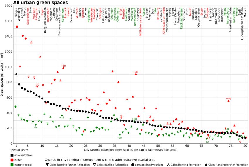
H. Taubenböck et al. Computers, Environment and Urban Systems 89 (2021) 101687
experiment with methods to better assess current urban conditions by rely on quantitative spatial parameters. Data are applied from citizen
the use of technology-based quantitative analysis. In this sense, our goal science approaches, e.g. for the assessment of resilience of green spaces
is to objectify a ranking through a multi-layered approach based on (Pudifoot et al., 2021), from official governmental data or by remote
remotely sensed data, without denying the ambiguities of statistics. sensing (Shahtahmassebia et al., 2021). A variety of measures are
One strategy to give the city a positive image is to highlight statistics applied such as green space accessibility, green volume, green space
of spatial indicators. Green spaces, as an example, have widely positive proportion or green space provision (e.g. BBSR, 2018; Fuller & Gaston,
connotations in society. In Germany, for instance, the cities of Berlin, 2009; Grunewald et al., 2018; Gupta, Kumar, Pathan, & Sharma, 2012;
Bonn, Halle (Saale) or Hanover take advantage of this and use the ad Morgenpost, 2016; Richter, Grunewald, Meinel, & Urbane, 2016).
jective ‘green’ in relation to their city to build a positive image. Hanover Overall, however, it has to be stated that spatial knowledge about the
even promotes itself as Germany’s greenest city. This branding, how green stock is still often insufficient which is an obstacle for Derudder
ever, remains statistically unquestioned, as long as this interpretation is and van Meeteren’s (2019) call for experimenting with technology-
accepted as plausible by society. It is precisely this unquestioned aspect based spatial analyses. On the one hand spatial data are often neither
that we examine in this study and which we underpin with quantitative available in the necessary spatial extent, the thematic or spatial detail,
statistics on urban green space shares. For this purpose, we present the needed accuracy and consistency, nor the desired up-to-dateness. In
multiple approaches of city rankings of the proportion of green spaces in Germany, as example, the federal area statistics based on the real estate
major German cities. On the one hand, this allows to show to what cadaster do show parameters for green areas, but their temporal and
extent the described perception of these four exemplary cities is also spatial consistency and nationwide availability is currently limited. On
statistically reliable in spatial terms. On the other hand, this allows to the other hand, the spatial indicators or measurement methods, which
systematize and discuss statistical ambiguities, which is created by the permit an evaluation, are neither obvious nor unambiguously defined, i.
choice of parameters and their conceptualization, and the spatial e. the comparison of spatial green indicators is not trivial.
reference units. In recent years, remote sensing has become a crucial data source for
In this study, we pick the parameter ‘urban green’ as example. Green the classification of green areas and it allows to work over large areas in
spaces, of course, have vital relevance for cities beyond perception and a consistent manner (e.g. Lamchin et al., 2020; Richards & Belcher,
branding. They play a crucial role in urban ecosystems: they allow 2020; Shahtahmassebia et al., 2021). Methods for deriving green spaces
rainwater infiltration refilling groundwater (e.g. Bolund & Hunhammar, based on remotely sensed data have advanced significantly even in the
1999; Wolch, Byrne, & Newell, 2014) which improves resistance to complex and small-scale urban landscapes (e.g. Parmehr, Amati, Taylor,
flooding (Banzhaf & De La Barrera, 2017). Cooling effects (evaporation, & Livesley, 2016). Approaches on very high-resolution (VHR) data with
shading, fresh air corridors, etc.) could be empirically demonstrated spatial resolutions of 1 m and better combined with three-dimensional
(Reis & Lopes, 2019) and thus the potential to mitigate the effects of data (e.g. LIDAR) allow a highly detailed recording of vegetated areas,
climate change to which urban flora, fauna and humans are increasingly green volume estimates or different vegetation species (e.g. Tooke,
exposed (BMUB, 2017). And, they contribute to biodiversity within Coops, Goodwin, & Voogt, 2009). The limitation for these VHR appli
cities as habitats for flora and fauna (Aronson et al., 2017; BMU, 2019). cations is primarily the limited possible spatial coverage, due to data
Green spaces also play a crucial role for urban citizens: In this context, cost and availability. In contrast, large-scale approaches with free-of-
the material resources of a city can be seen as a foundation through cost data are more limited in their spatial and thematic resolution.
which society is specifically constituted (Löw, 2008). In particular, Nevertheless, very good classification accuracies have been achieved
green areas provide spaces for recreation, social interaction and physical with sensors such as Sentinel-2 (e.g. Weigand, Staab, Wurm, & Tau
activity that have a positive impact on the mental and physical health of benböck, 2020) or Landsat (e.g. Pflugmacher, Rabe, Peters, & Hostert,
humans (Bertram & Rehdanz, 2014; TEEB, 2011). They are known to 2019) using shallow machine learning techniques. Lately, new image
reduce mortality and the risk of cardiovascular and respiratory diseases classification methods such as semantic segmentation from convolu
(Gascon et al., 2016; Weigand, Wurm, Dech, & Taubenböck, 2019). And, tional neural networks have proven very high accuracies for the detec
the design and quantity of greenery impacts on the visual character and tion of small-scaled structures in complex urban environments (Wurm,
perception of the urban landscape (Chmielewski, Bochniak, Natapov, & Stark, Zhu, Weigand, & Taubenböck, 2019), and have also been suc
Wężyk, 2020). With it, they contribute to the improvement of life cessfully applied for urban green spaces (Albert, Kaur, & Gonzalez,
satisfaction (reduction of stress, aesthetic experiences, spiritual enrich 2017). In this study, we therefore use Sentinel-2 satellite data instead of
ment) (WHO, 2016). indicators from the area statistics, which are prone to errors due to
In a world that is urbanizing at highest dynamics (Taubenböck et al., changes in the survey method. In this way, we aim to ensure compara
2012; UN, 2018), a balanced combination of built and natural urban bility across cities.
landscapes is increasingly important. With rising numbers of people In the field of spatial parameters for analyzing and comparing the
living in cities, the pressure on urban ecosystems and the environment green stock across space or over time, concepts, methods, thematic
increases. Land consumption is rising, for instance, as more space is content, spatial reference units, among others vary. We want to illustrate
required for living, commerce or traffic. Exposure to noise or air pollu these methodological particularities with the example of spatial refer
tion increases (Gómez-Baggethun et al., 2013; Grunewald, Xie, & Wüs ence units: Whatever the intended statement in studies analyzing urban
temann, 2018). The more important cities become as a living space, the green is (as done by Bertram & Rehdanz, 2014, Fuller & Gaston, 2009;
more important become urban living conditions. Initiatives, such as “Die Grunewald, Richter, Meinel, Herold, & Syrbe, 2016; Larondelle &
Grüne Stadt” (transl. “The Green City”) and public petitions (e.g. Haase, 2013; Richter, Behnisch, & Grunewald, 2017 or Richter et al.,
“Grünflächen erhalten” (transl. “Preserve green spaces”) in Munich) 2016; Kabisch, Strohbach, Haase, & Kronenberg, 2016), in most cases
show how not only decision-makers, but also the general public are indicators are developed on administrative reference units. While these
becoming increasingly aware of these issues and the protection of green units form the basis for political decision-making, in a geographic sense
spaces is a key concern (Bürgerbegehren Grünflächen erhalten, 2019; their historically and politically drawn boundaries do not make them an
Die Grüne Stadt, 2019). admissible basis for consistent comparisons. The modifiable area unit
In theory, a city ranking could be based on manifold parameters or problem (MAUP) testifies to aggregation effects on zonal statistics as
methodological approaches. Qualitative studies compare or evaluate the well as on size effects (Openshaw, 1983). These have been found to be
‘urban green’ e.g. by visual assessments on greening, questionnaires on scale dependent and nonstationary over space (Margulies, Magliocca,
subjective perception or parameters such as green quality (e.g. Ellaway, Schmill, & Ellis, 2016) and are prone to distort or even obscure reality
Macintyre, & Bonnefoy, 2005; Giles-Corti et al., 2005; Hoehner, (Taubenböck, Standfuß, Klotz, & Wurm, 2016). To address these chal
Brennan Ramirez, Elliott, Handy, & Brownson, 2005). Other approaches lenges in part with respect to the example of spatial reference units,
2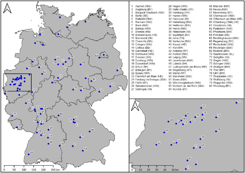
H. Taubenböck et al. Computers, Environment and Urban Systems 89 (2021) 101687
approaches have been developed to spatially separate cities from their potential benefits in terms of provisioning, regulating, habitat-shaping
surrounding areas in a consistent manner to provide an admissible and cultural services. With respect to climate-relevant effects, some re
spatial unit for cross city comparisons (e.g. Dijkstra & Poelmann, 2014; searchers state that regulating services, such as cooling the environment,
Melchiori et al., 2018; Taubenböck et al., 2019). Nevertheless, these are only provided by green spaces of one hectare or more (Arlt et al.,
approaches also carry conceptual challenges (e.g. border effects); a 2005; Finke, 1994). Thus, we conduct our analysis for all green spaces per
universal approach is non-existent. city and in addition also only for green spaces larger than one hectare.
Against this background, we aim in this study to systematically
compare the green stock in major German cities. The focus of our in 3. Study areas, geodata and spatial parameters
terest is on the structural differences and commonalities between cities.
To do so, we generally rely on classified green spaces derived from 3.1. Study areas: major German cities
remote sensing data. In contrast to other studies, we aim to develop a
city ranking that is fed by different urban green parameters and different The selection of the study areas is based on the need for an up-to-
spatial statistical perspectives. Based on a spatially variable multi- date, large-area, consistent geodatabase of spatially high and themati
subject concept, sufficient empiricism and a consistently conducted cally appropriate resolution. Since this is available for Germany (cf.
methodology, we aim to contribute to a more holistic, reliable Section 3.2), we include for our analysis all German cities which are
comparative urban research. In this way, we want to reduce the lack of ‘large cities’ by definition (Fig. 1). These are 80 cities which have at least
empirical knowledge about the positioning of different cities in a rela 100,000 inhabitants (BBSR, 2018). The data of the German Federal
tional field, as demanded by Löw (2008). Statistical Office served as a basis for the selection and they refer to
December 31st 2017 (DeStatis, 2020). This population information was
2. Conceptualization of the study assigned to grid cells with a side length of 100 m in an INSPIRE
compliant grid (BKG, 2020). For the spatial definition of the respective
Green spaces are one (of many) important indicator to describe and city centers, we rely on the data sets provided by the German Federal
evaluate urban living conditions and quality of life. Related statistics Agency for Cartography and Geodesy (BKG) (BKG, 2020).
often serve as a basis for societal debates or political decision-making.
Spatial statistics, however, are always prone to ambiguity – which pa 3.2. Geodata: green spaces
rameters are used, which scale of analysis is applied, how accurate or
consistent are input data, or to which spatial reference unit is the In this study we rely on green spaces classified from Sentinel-2 sat
measurement referred to. And with that, we run the risk that ill- ellite data. This data is free of cost and features area-wide coverage with
considered spatial statistics either lead to a random result or are a high spatial resolution of 10 m ground sampling distance. The acqui
selected specifically to achieve certain results, which are then to serve as sition period of the images for the classification was between 2015 and
the basis for political decisions. 2017, i.e. the classification is based on data that were not recorded at the
In this study we build a relational reference system of cities with same time. The classification algorithm was trained for seven thematic
respect to green spaces. It is intended to offer more resilient results land-cover classes: artificial land, open soil, high seasonal and perennial
through multiple perspectives. Our focus is on two common parameters vegetation, low seasonal and perennial vegetation as well as water.
in this field: The proportion of green space and the provision of green space Artificial land relates to built-up areas, low seasonal vegetation com
per capita. Both parameters are calculated relative to area or number of pares to croplands, low perennial vegetation features pastures, vine
inhabitants and are thus basically suitable for comparisons of cities of yards, and orchards, high seasonal vegetation subsumes deciduous tree
different sizes. We choose the parameter ‘proportion of green spaces’ cover including forests and fruit tree crops, and high perennial vegeta
because a comparable study by data analysts from Morgenpost (2016) tion relates to evergreen tree cover (cf. nomenclatures in alignment with
used exactly this parameter for their ranking. And we rely on the Anderson, Hardy, Roach, and Witmer (1976)). Fig. 2 illustrates the
parameter ‘provision of green space per capita’ as it is recognized and classification for two sample cities, Karlsruhe and Dresden. The classi
used by the World Health Organization (WHO, 2010). Our scale of fication features an overall accuracy of 93.07%. Details on data,
analysis is the city level. However, in our conception, we do not want to methods and results are shown in Weigand et al. (2020).
conceive the city (or its spatial extent) here as a given territorial unit. Green spaces are heterogeneous not only in their spatial distribution,
Rather, we vary the spatial reference units defining the city extent in but also in their phenological characteristics, as already indicated in the
order to gain a deeper understanding of green space proportions. Our classification scheme. This means that a green space can be low seasonal
starting point is on administrative reference units, which is the spatial vegetation (such as shrubland), high perennial vegetation (such as de
entity that is commonly used and the legal basis for decision-making. In ciduous forest), among others. In our analysis, we do not differentiate
addition, we elicit how consistent results are when we change the spatial here. We aggregated the various vegetation classes into one thematic
reference unit. For this purpose, we use a morphological spatial unit that class: green areas. This abstracts our input data but also makes them
encompasses the built space of a city and a standardized radius-based consistent, so that a comparison is feasible.
buffer unit around the center. Our input data are based on one consis
tent data source: remote sensing data. Thus, we rely on a consistent and 3.3. Spatial reference units
full survey without distinguishing between public and private green
spaces. The data set has a transparent assessment of accuracy and the Typically, city rankings are based on administrative boundaries.
original data sets have a high spatial resolution. These spatial units are crucial as they determine a clear-cut city’s
Our study focuses on the systematic comparison of cities in terms of boundary to establish jurisdictional competence of its municipal gov
spatial green shares. We relate cities to each other as we believe that ernment (Parr, 2007). Therefore, we use them as a starting point in our
they are a conceptually similar target entity. For this purpose, we use city analysis. We rely on administrative boundaries as provided by BKG (BKG,
rankings as a means of choice. In general, we imply higher spatial shares 2020).
and larger entities of green spaces are related to a higher likelihood of However, these administrative units form an artificial unit as they
positive effects (e.g. Arlt, Hennersdorf, Lehmann, & Thinh, 2005; Gill, have been created by very different political and historic developments.
Handley, Ennos, & Pauleit, 2007). On the one hand, this means that we Although often applied, they do not form a consistent and thus com
set the city with the highest share in the ranking to one. On the other parable spatial entity for city comparisons from a geographic point of
hand, we consider that the size of an urban green area is of great view (Taubenböck et al., 2019). It has been shown that the zonation
importance for their effects: The larger the green space, the higher its effect, i.e. a re-arrangement of a spatial reference system into different
3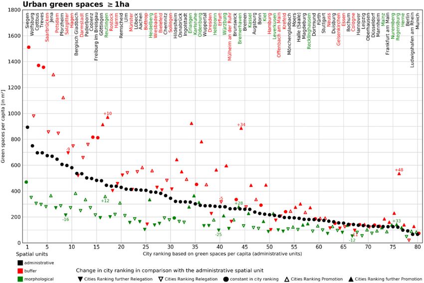
H. Taubenböck et al. Computers, Environment and Urban Systems 89 (2021) 101687
Fig. 1. Selected German cities with corresponding Federal state: BB = Brandenburg, BE = Berlin, BW = Baden-Wuerttemberg, BY = Bavaria, HB = Bremen, HE =
Hesse, HH = Hamburg, MV = Mecklenburg-Western Pomerania, NI = Lower Saxony, NW = North Rhine-Westphalia, RP = Rhineland-Palatinate, SH = Schleswig-
Holstein, SL = Saarland, SN = Saxony, ST = Saxony-Anhalt, TH = Thuringia.
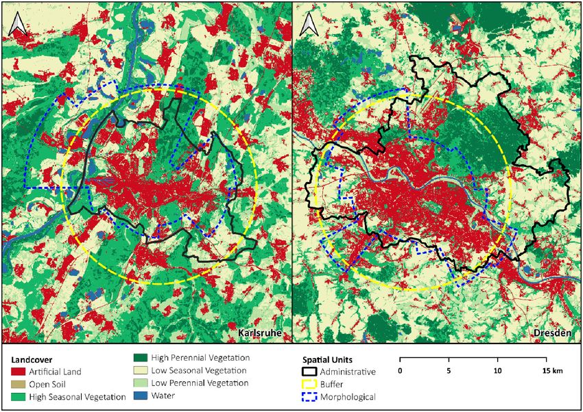
Fig. 2. Land-cover classification and three different spatial reference units delineating the entity city differently for the examples of Karlsruhe and Dresden.
4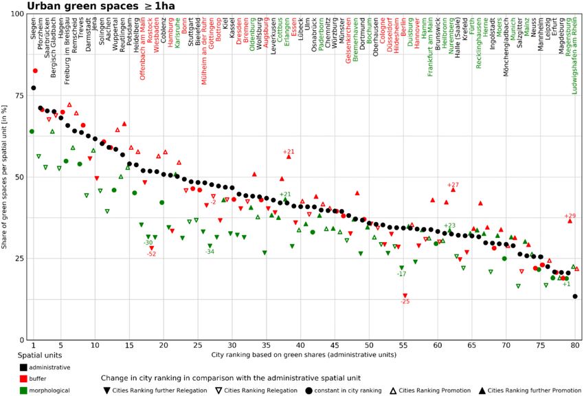
H. Taubenböck et al. Computers, Environment and Urban Systems 89 (2021) 101687
units, may lead to – although based on the same initial values – different climate-relevant green spaces larger than 1 ha, and the three spatial
results and conclusions (Jelinski & Wu, 1996; Madelin, Grasland, reference units, overall twelve different city rankings are possible. This
Mathian, Sanders, & Vincent, 2009). alone shows the diversity of spatial statistics.
Against this background, we apply two other spatial reference units In deconstructing this variability, we adopt the following rationale:
that are supposed to also mark the entity ‘city’: a buffer and a morphologic We first rank the cities based on their green space shares (total and per
unit. capita), i.e. the highest share is number one. We use the city ranking
The buffer unit is understood as a uniform unit, independent of city based on the administrative spatial units as a starting point and analyze
sizes or spatial patterns. Here we apply a standardized buffer, using a 10 the deviations in the other spatial units. To show the differences be
km radius around each city center. The selected circle and radius are tween the results statistically, we determine the correlations between
here representative for other possible spatial units like squares or rect the approaches and describe their relationship through the coefficient of
angles, or other radii. The point here is simply to incorporate a uniform determination. We illustrate city sizes in these correlations in order to
size and shape as an example, as one possible variant of consistent relate trends in green space shares to city sizes.
geographic comparison. Since there are cities included in the analysis In order to identify cities with higher rank changes across spatial
which are located in close proximity in highly agglomerated areas, such units, we classify them according to the comparison to administrative
as the Ruhr area (Fig. 1), in some cases the buffer units of different cities ranks, i.e. in those that feature above average rank losses in comparison
overlap. However, in our analysis we treat each city individually, i.e. to administrative ranks (indicated in red in Figs. 4 and 5 as well as in
green spaces in overlapping situations are part of the analysis for both Figs. A and B in the Appendix), and vice versa the ones with above
cities. average rank gains (indicated in green in Figs. 4 and 5 as well as in
Both spatial units, the administrative and the buffer unit, do natu Figs. A and B in the Appendix). The classification is based on the average
rally not capture the morphologic settlement extent of cities in a perfect of the changes in ranks for morphological and buffer units. All mean
sense. Therefore, we introduce a morphologic unit as a third spatial entity. values above the respective median are classified as cities with higher
It is our basic assumption that boundaries of the city are conceptually changes in rank.
difficult to determine (Sievers, 1997), but in principle they exist. To Rankings are naturally also based on the desire to be able to make
address this concretely, we apply an approach that delineates cities as a simple and clear statements and classifications. However, the diversity
spatially coherent, comparatively dense built-up landscape. Using of the conceptually and methodologically reasoned variety of results
remotely sensed classifications on built-up structures and their density, contains a complexity that makes a simple answer to our guiding
the city boundary can be determined along an urban-rural gradient in a question “which is the greenest city?” difficult. Thus, we generate a final
data-driven way (cf. for methodological details Taubenböck et al., result to meet both challenges: to abstract and simplify this complexity
2019). Based on a monocentric city model, it is assumed that with to make a clear statement by benchmarking cities in one final ranking,
increasing distance from the city center, the transition from urban to but at the same time not without quantifying the uncertainties in the
rural is along a decreasing built-up density (Fig. 2). As it is impossible to process. Therefore, we merge all twelve rankings into one single
distinguish the urban from the rural according to a universal truth, the ranking. To do this, we use all twelve ranks per city and list them
strength of this approach lies in its consistency, i.e. for all test cities the descending over their mean value, with the lowest total in first place and
boundaries are set in a mathematically unambiguous, consistent and the highest total in last place. We use standard deviations for the ranks to
thus comparable manner. For some cities located in close proximity, the indicate the uncertainties. This way, we base the final result on all views
morphology units also do overlap. As for the buffer units, the same in equal parts.
assumption was made, that some green spaces are part of the statistical
analyses for two cities at the same time. 4. Results
Fig. 2 illustrates the three spatial units that variably constitute the
entity city in spatial comparison. In the example of Dresden, the Depending on the green parameters (green space share, green space
administrative unit includes the Dresdner Heide, a large forest area in share >1 ha, green space per capita, green space >1 ha per capita) and
the north-east of the city center. The morphological boundary, in the spatial units (administrative, buffer, morphologic) used, results vary.
contrast, draws the border tightly around the built city and thus the First, we introduce some general results in an overview and secondly, we
Dresdner Heide is not part of the spatial reference unit – with corre present the city rankings.
sponding consequences for the green share.
4.1. General results
3.4. Spatial parameters on green space shares
For the aggregated results from our sample of 80 major cities in
In this study we apply a quantitative approach, since we rely on Germany, we highlight the following key statistics: For the three spatial
consistent data sets for green space shares as well as for city populations reference units applied, we measure differences in size and extent. In
for all cities. We base our city ranking on two quantitative parameters: comparison to the common administrative units, the morphological
(1) Green space proportion, i.e. the share of the total green space relative boundaries draw the city boundary more tightly around the built-up
to the total reference area calculated in percent. Although this metric space, i.e. this reference unit is on average smaller. Specifically, 56 of
merely reflects the quantity of green space and not its quality, it is a our 80 sample cities are smaller, by an average of nearly 33 km2. In
parameter often applied as proxy for evaluating the quality of the urban contrast, the standardized buffers of 10 km radius predominantly
life and the ecosystem (BBSR, 2018; Faryadi & Taheri, 2009; Morgen encompass the administrative city units: 75 of the 80 city entities are
post, 2016). (2) Green space provision per capita, i.e. the total green space larger, by an average of almost 142 km2 more area. These differences in
available for each citizen calculated in m2 per person. This measure is extent, of course, have an impact on the population figures covered by
often used in the political decision-making process. The WHO, for these spatial reference units. On average, over 138,000 more people live
instance, calls for a minimum of 9 m2 of urban green areas per inhabitant in the buffers than in the administrative units. It is remarkable that
and defines 50 m2 per capita as desirable (WHO, 2010). morphological boundaries, although smaller on average, still hold
nearly 50,000 more people on average than administrative units. This
3.5. City rankings and their deconstruction effect is mainly related to the cities in close proximity with a continuous
built landscape, whose morphological units cover areas that belong to
With the two parameters on green space shares, the two-dimensional administratively different cities.
distinction according to spatial extent between all green spaces and the If we now look at the parameters, i.e. the (1) green space shares and
5
H. Taubenböck et al. Computers, Environment and Urban Systems 89 (2021) 101687
(2) green space per capita aggregated across all cities, we measure the have higher proportions).
following differences to administrative units: (1) morphological The statistical relationship of the different parameters and spatial
boundaries with their smaller extents result in green space shares that units generally reveal good linear fits with coefficients of determination
are on average 6.8% lower (− 7.2% for green areas >1 ha). 67 of the 80 between 0.644 and 0.784 (Fig. 3). While this may be considered a good
cities have a lower green space share on this reference unit. This reveals correlation in principle, it shows that the spatial units do have a strong
that administrative units usually integrate more natural and close-to- influence on our result. The different spatial units all have similar spatial
nature areas around the actual built space and therefore green pro bases, i.e. the city center and more or less the contiguous built-up areas,
portions are higher. Buffer units, although spatially very different from but they are drawn very differently at the edges of the cities, sometimes
administrative boundaries, have similar green space shares on average narrower, sometimes wider. And the fact that this alone is enough to
(− 0.4% and − 0,2% for green areas >1 ha), but basically it is distributed have coefficients of determination of only 0.644 shows how fragile
indifferently here. 35 cities have higher proportions and 45 have lower spatial statistics can be. Especially in the case of green space per capita
proportions. This shows that this spatial unit is neither adapted to the and the morphological spatial units, we see immense deviations to lower
shape nor to the size of the particular city. (2) For the aggregated green values compared to administrative spatial units.
space shares per capita, we see fundamental differences in the statistics: With regard to available green spaces, a certain relationship to the
For the morphological units, the supply of green space per capita is size of the city can be identified. For cities that have very high green
decreasing on average by 140 m2 per capita (139 m2 for green areas >1 space shares, we exclusively see low population numbers within our
ha) (and 71 of the 80 cities have falling figures) compared to adminis sample. Vice versa, the cities with large populations such as Berlin or
trative units (on average 331.7 m2). For the buffer units (on average Munich (larger cities are indicated in red and orange colors in Fig. 3)
475.4 m2), on the other hand, the provision per capita increases by 144 show low green shares. This inverse relationship is even more pro
m2 per capita (+141 m2 for green areas >1 ha) (and 64 of the 80 cities nounced when looking at green space per capita.
Fig. 3. Relationships of spatial green shares and green spaces per capita for morphologic and buffer units to the reference values based on administrative units. All
cities are classified using population numbers. (For interpretation of the references to colour in this figure legend, the reader is referred to the web version of
this article.)
6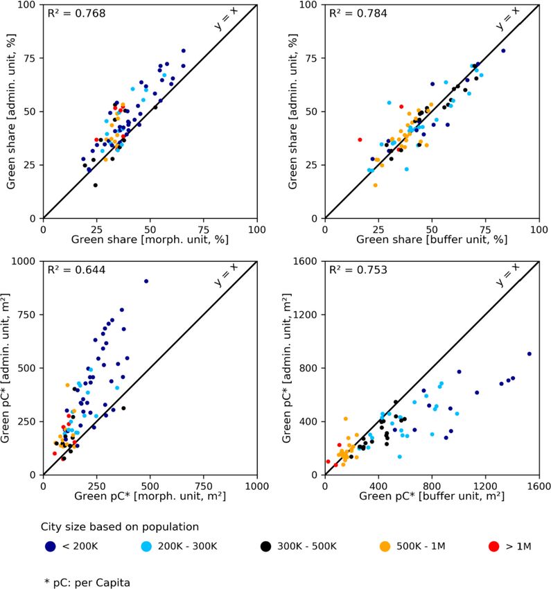
H. Taubenböck et al. Computers, Environment and Urban Systems 89 (2021) 101687
4.2. The city rankings Fig. 4 illustrates the rankings among all 80 cities for the green space
shares at administrative reference units. It reveals deviations in the
As variable as the parameters on urban green in relation to the ranking based on the alternative morphologic as well as on the buffer
different spatial units are, one thing remains indisputable according to units.
our city ranking analyses: The city of Siegen can claim to be the greenest Basically, it can be stated that the ranking for the different spatial
large city in Germany (cf. Figs. 4 and 5). In every ranking except for one, units varies. It is interesting to note that 34 cities register strong changes
this city is ranked number one (green space shares for administrative/ in the ranking – 15 cities generally fall back in rankings, while 19 cities
buffer/morphologic units: 78.4%/83.4%/65.6%; green areas >1 ha: rise. For example, the city of Wiesbaden ranked 19 for green space
77.3%/82.6%/63.9%; green area per capita: 906 m2/ 1526 m2/ 482 m2; shares on administrative spatial units (53.1%) drops by 35 ranks on
green areas per capita >1 ha: 894 m2/ 1511 m2/ 470 m2). Siegen is morphologic units (33.6%). Or the city of Recklinghausen ranked 62 on
second only in the ranking of the morphologic units on green areas >1 this parameter on administrative units (34.4%) gains 27 ranks with
ha, with Bergisch-Gladbach slightly overtaking Siegen with 64.0% morphologic units (36.7%). Without judging or evaluating what is true,
compared to 63.9%. these examples illustrate that statistics can make cities rank much better
The situation is more ambiguous with regard to the last place in the or worse depending on the calculation method.
ranking. Here, the cities of Ludwigshafen (administrative units: green We observe the same effects regarding the ranking based on the
space shares 23.6%; green areas >1 ha 13.5%; green areas per capita >1 green spaces per capita (Fig. 5), here 35 cities register strong changes in
ha: 67 m2), Munich (administrative units: green areas per capita: 74 m2), the ranking: An extreme example is the city of Erfurt. On an adminis
Berlin (buffer units: green space shares: 16.4%; green area per capita: 24 trative spatial unit, it offers over 300 m2 of green space per capita. On a
m2; green areas >1 ha: 13.6%; green areas per capita >1 ha: 20 m2; morphological unit, however, it only has 114 m2 and falls 25 places
morphologic units: green area per capita: 54 m2; green areas per capita (from 37 to 62) in the ranking. Vice versa, Regensburg is an example in
>1 ha: 48 m2), and Salzgitter (morphologic units: green area shares: the opposite direction: on morphological units this city gains 31 ranks
18.8%; green areas >1 ha: 16.6%), alternate. (from 74 to 43) and increases its per capita green share from 136 m2 to
In general, we can state the range of green space shares in German 160 m2 compared to the statistics on the administrative level.
cities is very uneven. To pick just two examples: the range of green area In the Appendix, Fig. A analogously presents the ranking for green
shares between 1st and 80th place is 62.9% at the administrative level, spaces larger than 1 ha and Fig. B illustrates the ranking for green spaces
on the morphologic unit it is less with 46.8%, but still remarkably high. larger than 1 ha per capita.
The tangible effects on the individual person become clear in the second In a final attempt to create one final ranking that is as holistic as
parameter: the range between 1st and 80th place for green space shares possible to abstract and simplify this complexity in rankings, we
per capita are 832 m2 at the administrative level, on the morphologic combine all the ranks of the 12 individual city rankings (Fig. 6). Thus,
unit it is with 428 m2 again less. While this is an indication that the with regard to the two parameters ‘green space shares’ and ‘green space
figures of the morphological delineation are more comparable due to the provision per capita’, the two variants according to spatial extent ‘all
data-driven approach, we can state that green space provision across green spaces’ and ‘green spaces larger than 1 hectare’, as well as the
German cities varies immensely. three spatial reference units, it can be said that Siegen is undoubtedly
Fig. 4. Proportion of green spaces in German cities at three different spatial units: administrative, buffer and morphological. The cities are ranked along the x-axes
for administrative units and deviations in the ranking are marked for the buffer as well as the morphological units. City names are classified by above average rank
loss (red) and above average rank increase (green) relative to administrative units. (For interpretation of the references to colour in this figure legend, the reader is
referred to the web version of this article.)
7
H. Taubenböck et al.                                                                                           Computers, Environment and Urban Systems 89 (2021) 101687

Fig. 5. Proportion of green spaces per capita in German cities at three different spatial units: administrative, buffer and morphological. The cities are ranked along
the x-axes for administrative units and deviations in the ranking are marked for the buffer as well as the morphological units. City names are classified by above
average rank loss (red) and above average rank increase (green) relative to administrative units. (For interpretation of the references to colour in this figure legend,
the reader is referred to the web version of this article.)

Fig. 6. Final ranking of the 80 largest German cities with respect to green area shares from the combination of all rankings and their standard deviations. (For
interpretation of the references to colour in this figure legend, the reader is referred to the web version of this article.)

and unambiguously the greenest of all large cities in Germany. This                    cities such as Berlin, Munich, Cologne or Hamburg.
position is also reflected in the gap to the second place (Pforzheim).                     Within this relational field generated from twelve rankings the
Ranks two to eleven are occupied by cities such as Treves, Saarbrucken                 probability of being subject to method-specific coincidences is lower,
or Potsdam – all of which tend to have smaller population numbers in                   but the standard deviations indicate related uncertainties. For some
our sample. At the lower end of the ranking we find many of the larger                 cities the standard deviations are low or relatively low (especially at the

                                                                                   8
H. Taubenböck et al. Computers, Environment and Urban Systems 89 (2021) 101687
top as well as at the lower end of the ranking). With it their positioning is the operational measurement of green space shares is subject to con
generally stable and less guided by spatial statistical coincidences (e.g. ceptual and methodological specifics and can therefore be manipulated.
Siegen, Coblenz or Mannheim). In contrast, some cities (e.g. Salzgitter, From the perspective of our input data, the remotely sensed data are a
Rostock or Regensburg) feature very high standard deviations and their consistent database and feature a generally high accuracy of 93.07%,
positioning is prone to methodological specifics. This can be taken as an which makes our results robust. Nevertheless, we have to note that the
indication that the local specifics, i.e. e.g. spatial patterns of the city or spatial resolution of 10-m pixels does lead to challenges in specific
city sizes, must be particularly considered here for a precise estimation. structural environments. In areas of large parks or forest areas, our
classification even achieves higher accuracies. However, in small-scale,
5. Discussion complex structures (e.g. detached houses with small gardens), we come
up against limits with spatial resolution. Here we also measure lower
In order to see one’s own, comparison is required. One way of accuracies. Accordingly, since many areas in cities have this complex
assessing oneself is within a relational system by means of a ranking. So, structural composition, it can be assumed that certain measurement
whether a city is well or poorly equipped with green spaces is not easy to inaccuracies show through and have an unknown, although probably
assess in absolute terms, but to classify in comparison. However, there not significant, effect on our ranking.
are a wide variety of challenges and pitfalls to permissible and mean
ingful comparisons. We now critically review methods and data used to 5.2. Reflections on the rankings
compile our rankings, we reflect on rankings in general and suggest a
strategy for more scientifically sound rankings, and finally we discuss Our results of various city rankings with respect to green spaces
the geographical results of this study. show, first of all, that there is no absolute truth. There is no one right
parameter or no one right spatial reference unit. We argue here that
5.1. Reflections on methods and data achieving a higher reliability in benchmarking a city within a relational
system is only possible through manifold methodological variants. And
As we have seen in this study, the choice of methods and data in still, although the various empirical approaches presented are system
fluences the resulting rankings to a not insignificant degree. In this atic, it is not possible to produce a simple or universally valid ranking.
context, we discuss the applied parameters, spatial units and accuracies And it is precisely this that exposes pitfalls of rankings. In scientific
of the input data. literature, city rankings are often criticized, from an epistemological
In terms of parameters, we have relied on two accepted measures, point of view as well as from the ideology behind them (White & Kitchin,
‘green space shares’ and ‘green space shares per capita’, each also ac 2021). Therefore, as critically discussed by Acuto et al. (2021), any
cording to ‘all green spaces’ and to ‘green spaces larger than 1 hectare’. ranking must be critically questioned in terms of how it came about, who
This decision is not based on the fact that these parameters are the most makes it, what it represents, and who it influences.
relevant, but rather due to the need for consistent, comprehensive and The challenge that despite a uniform data basis and consistent cal
appropriate geoinformation. We are aware that these parameters can be culations, rankings (in our case on green shares) vary due to the different
expanded almost arbitrarily (e.g. green volumes, green space types, or choice of parameters or spatial reference units is shown in this work.
quality), if the data situation allows, and that this would even create This explains to some extent why there is neither a scientifically
more variability in rankings. It also remains to be considered that the approved benchmark for urban green spaces nor are there generally
quantity of green spaces measured in this study, does not equal quality. accepted survey and measuring methods. In Germany, only some
In this sense, we must be aware that it is not only quantity but also the orientation values, parameters and indicators are defined for individual
respective spatial patterns which have effects on ecological or social urban districts without general validity (BBSR, 2018). And yet, ac
functions, i.e. whether green spaces are more spatially clustered, large, cording to Kitchin, Lauriault, and McArdle (2015), rankings are attrac
and contiguous or more distributed, small and dispersed. tive to practitioners because they offer a semblance of technocratic
In terms of spatial units, the administrative unit is crucial, as it forms objectivity and satisfy the need for political expediency. And, rankings
the spatial basis for planning and political decisions. At the same time, have become a central tool of intercity competition.
the administrative entity distorts the statistics because these spatial Therefore, this work intends to contribute to the objectification of
reference units are not consistent across cities. For this reason, we have rankings. We believe that the presented multi-layered ranking allows a
introduced morphological units. These are based on a data-driven more objective and stable positioning of cities within a relational com
delineation of the built environment from a remotely sensed classifica parison system. Through conceptual and methodological diversity, it
tion. Therefore, we consider them to be a consistent spatial baseline for makes rankings less susceptible to corresponding randomness and the
comparing cities. The built urban space is here predominantly more representation of uncertainties allows to overcome absoluteness in
narrowly delineated around the built urban environment than admin rankings. Thus, this multi-layered approach can indicate, via un
istrative units and, hence, the actual amount of green space available certainties, whether local specifics need to be considered when devel
within the built city can be determined. However, it is also clear that this oping interventions strategies. But we must be aware, that even this
approach simultaneously negates green spaces in the close vicinity of the multi-layered approach cannot create complete unambiguity in the
built landscape. And, as a third, supplementary spatial unit, we have ranking. The combination of twelve variants in this work is thus inten
added a constant area in terms of a buffer unit of 10 km around the city ded to provide a blueprint that can be extended at any time to include
center. We believe, this unit allows to determine green space shares additional green parameters.
beyond the built space and to compare them permissibly on the basis of The combination of the various rankings allows us to undoubtedly
the same extent for all cities. However, the buffer unit is very artificial designate Siegen as the greenest city in Germany. This is first of all a
because it does not take the spatial pattern or size of the city into ac confirmation of a similar result of a methodologically different study a
count. Nevertheless, this unit adds an additional perspective on green few years ago (Morgenpost, 2016). However, only one parameter and
space shares in space that can contribute to the overall view as done in one measurement method were used in their study. While the same
the merged ranking. In general, we should also be aware that these two study provides an equally clear result regarding the last place (Lud
spatial units, morphologic and buffer units, could also be permuted by wigshafen), we paint a more complex picture here due to the un
other radii or shapes, or by alternative spatial definitions of city centers. certainties (Ludwigshafen, Munich, Berlin, Salzgitter). This means that
Effects of these variants have been shown (e.g. James et al., 2014); secondly, in our study the challenge and the potential lies rather in the
however, the effects to our rankings have not been tested in this study detail of data interpretation. Whether Siegen has 65,6% (morphologic)
and must remain unknown. This once again demonstrates in general that or 83,4% (buffer) green space shares or whether it provides 482 m2
9H. Taubenböck et al. Computers, Environment and Urban Systems 89 (2021) 101687
(morphologic) or even 1526 m2 (buffer) green spaces per capita – so in with less spatial quantity. For compensation in the social sphere, high
fact very different values that can be attributed to a city – depends on the quality and accessibility can be more important than quantity in certain
spatial reference unit applied. These variabilities in numbers reveal the cases. Last but not least, it must also be borne in mind that in the struggle
complexity of a reasonable assessment of the situation and a good for urban space, never only one parameter (in our case green areas) must
strategy of evaluation cannot emerge by a more or less randomly chosen be considered whether a city is liveable. This is always linked to the need
approach, but only in a differentiated view: an evaluation that reflects for housing, infrastructure, culture, and much more. The fact that many
conceptually and methodologically and co-evaluates local specifics in of the larger cities such as Berlin, Munich or Hamburg are at the bottom
individual cases to derive appropriate recommendations for action. of the ranking also makes the following clear: these cities are highly
And in this sense, benchmarking can be a valuable tool to develop sought-after residential locations in Germany with highest influxes or
and address constructive interventions and to contribute to the strate highest (and increasing) housing prices. Their attractiveness and the
gies of local governments (Robin, 2021). Whether and how local actors perception of qualities of place and life do not seem to be influenced in
can translate this knowledge into action and to what extent rankings in the least by the lowest proportion of green space among German large
general and this one in particular help to define interventions must, cities.
however, remain open at this point.
6. Conclusion
5.3. Geographical reflections
The question “what is the greenest city of Germany?” seems to be
From a geographical point of view, we can generally state from our trivial. Nevertheless, behind this supposedly simple question lies a
analysis that German cities are well equipped with green spaces. When deeper complexity. True to the motto “don’t trust statistics that you
we relate our results to the suggestions of the WHO calling for a mini haven’t faked yourself”, our different experiments on the proportion of
mum of 9 m2 of urban green spaces per capita and defining 50 m2 per green spaces in cities are not ‘fakes’, but transparent in their parameters,
capita as desirable (WHO, 2010), we see that even the cities at the data and methods, and still nothing is black or white. Based on con
bottom of the ranking are (at the administrative unit: Munich 74 m2 and ceptual definitions, applied parameters or spatial units of measurement,
at the morphological unit: Berlin 54 m2) equipped with even more green a myriad of statistics which are all mathematically correct, can be pro
space per capita than desirable. For the buffer unit, the green area space duced to steer the impression one or the other way.
per capita for the ranking tail end Berlin is 24 m2, which is about half of With this study we show how fragile spatial statistics are, but how
what was suggested as desirable. Herein this particular case we have to they can then be (mis-)used for political decisions without considering
consider that the 10 km radius for Germany’s largest city only covers the the complexity of reality. However, with manifold different perspectives
core city. Based on its green space shares on the morphologic (54 m2 per – according to parameters and spatial units – we believe we can
capita) as well as the administrative unit (100 m2 per capita), we see the contribute to a more holistic understanding for systematically
proposed minimum is far exceeded. approaching these issues. We argue here in the line of Derudder and van
With respect to the four example cities from the introductory section Meeteren’s (2019) call to engage with ‘urban science’: for expanding
– Berlin, Bonn, Halle and Hanover – which have branded themselves by this multi-layered ranking including related uncertainties in future sci
the adjective ‘green’, we observe something somewhat surprising: none entific work by experimenting with methods and technology-based
of the three cities is in the top 10 of our ranking or even close to it. Bonn quantitative spatial analysis to better assess current urban conditions.
is at rank 41 in the combined ranking, Halle at 65, Hanover, the self- The addition of alternative spatial approaches such as green components
proclaimed greenest city in Germany, ranks 74th, and Berlin even at in the immediate surroundings of households (Wüstemann, Kalisch, &
the penultimate position 79. Thus, the question arises whether this Kolbe, 2017) seems to be just as relevant as systematically integrating
attribute for branding is by any means justified. These claims can be further parameters such as urban green accessibility, size, edges, vol
attributed to the practice of “greenwashing” (e.g. Seele & Gatti, 2017), i. umes, spatial patterns or connectivity, among others to extend the
e. a form of marketing in which e.g. green statistics are used to convince suggested multi-layered concept of rankings.
the public that, in our case, the city stands out in particular. When As spatial thinking forces to think in difference, we believe being
relating our results to the marketing use, it seems that whether a city is able to describe and understand these differences between approaches
accepted as green in the public perception seems to depend less on as well as between cities in their complexity in a more holistic sense. We
objective spatial shares and more on what people accept as plausible. In see this as a starting point for thinking about urban developments. With
this sense, Bok (2021) points to the powerful influence of rankings in this basis of good empirical knowledge within a relational system, the
defining and narrating the normative conditions of discourse and prac necessity for constructive interventions can be identified, examples of
tice. This is, of course, accompanied by the need for objectification. others can be studied and planning attempts can be made to overwrite or
In our rankings, we have basically assumed that a higher share of to adapt the existing structures of a city.
green spaces is related to a higher likelihood of a positive effect (Arlt
et al., 2005; Gill et al., 2007). In this rationale, the purely quantitative Acknowledgments
approach in this study is justified, but of course, reality is more complex.
We should be aware, that the distribution of green spaces reflects the This study was partly funded by the German Federal Institute for
importance of the local. The impact of green areas is on the space that Research on Building, Urban Affairs and Spatial Development (BBSR)
encompasses everyday life or on cooling effects in the immediate vi (project “Monitoring des Stadtgrüns), the German Federal Ministry of
cinity, and that is something quite different than measured at adminis Transport and Digital Infrastructure (BMVI) (projects “meinGruen” and
trative (or other) units defining the city (Löw, 2008). In addition, we “SAUBER” (funding codes 19F2073B and 19F2064B, respectively)), and
should be aware that quantitatively fewer green areas do not necessarily by the German Federal Environmental Foundation (DBU). We would
have fewer positive effects: with suitable spatial arrangement or also like to thank Julia Tenikl and Lennart Imberg for their support.
different types of green areas, climate-relevant effects may be achieved
10You can also read