Object-based analysis of simulated thunderstorms in Switzerland: application and validation of automated thunderstorm tracking with simulation ...
←
→
Page content transcription
If your browser does not render page correctly, please read the page content below
Geosci. Model Dev., 14, 6495–6514, 2021
https://doi.org/10.5194/gmd-14-6495-2021
© Author(s) 2021. This work is distributed under
the Creative Commons Attribution 4.0 License.

Object-based analysis of simulated thunderstorms in Switzerland:
application and validation of automated thunderstorm tracking
with simulation data
Timothy H. Raupach1,2,a , Andrey Martynov1,2 , Luca Nisi4 , Alessandro Hering4 , Yannick Barton1,2 , and
Olivia Martius1,2,3
1 Oeschger  Centre for Climate Change Research, University of Bern, Bern, Switzerland
2 Instituteof Geography, University of Bern, Bern, Switzerland
3 Mobiliar Laboratory for Natural Risks, University of Bern, Bern, Switzerland
4 Federal Office of Meteorology and Climatology MeteoSwiss, Locarno, Switzerland
a present address: Climate Change Research Centre, University of New South Wales, Sydney, Australia

Correspondence: Timothy H. Raupach (timothy.h.raupach@gmail.com)

Received: 7 April 2021 – Discussion started: 28 May 2021
Revised: 12 August 2021 – Accepted: 28 September 2021 – Published: 27 October 2021

Abstract. We present a feasibility study for an object-based   1   Introduction
method to characterise thunderstorm properties in simula-
tion data from convection-permitting weather models. An        Convection-permitting simulations will play a critical role in
existing thunderstorm tracker, the Thunderstorm Identifi-      reducing the existing high uncertainty around the responses
cation, Tracking, Analysis and Nowcasting (TITAN) algo-        of thunderstorms (e.g. Diffenbaugh et al., 2013; Collins et al.,
rithm, was applied to thunderstorms simulated by the Ad-       2013; Hartmann et al., 2013; Allen, 2018) and hailstorms
vanced Research Weather Research and Forecasting (AR-          (e.g. Martius et al., 2018; Allen, 2018; Raupach et al., 2021b)
WRF) weather model at convection-permitting resolution         to climate change. Such models have sufficiently high reso-
for a domain centred on Switzerland. Three WRF micro-          lution to explicitly resolve individual storm structures with-
physics parameterisations were tested. The results are com-    out parameterised convection (e.g. Weisman et al., 1997;
pared to independent radar-based observations of thunder-      Bryan et al., 2003) and thus address thunderstorm initiation,
storms derived using the MeteoSwiss Thunderstorms Radar        which cannot easily be addressed if proxy relationships are
Tracking (TRT) algorithm. TRT was specifically designed        used to infer information about thunderstorm environments
to track thunderstorms over the complex Alpine topography      (e.g. Tippett et al., 2015). High-resolution simulations can
of Switzerland. The object-based approach produces statis-     be difficult to compare either to one another or to obser-
tics on the simulated thunderstorms that can be compared       vations, since mismatches in timing or location of weather
to object-based observation data. The results indicate that    features can occur even when the overall statistical proper-
the simulations underestimated the occurrence of severe and    ties of the weather phenomena are in agreement, leading to
very large hail compared to the observations. Other prop-      point-to-point comparison results that do not properly show
erties, including the number of storm cells per day, geo-      model performance (e.g. Ebert, 2009; Gilleland et al., 2010).
graphical storm hotspots, thunderstorm diurnal cycles, and     Object- or feature-based comparisons are one way to address
storm movement directions and velocities, provide a reason-    this problem (e.g. Ebert, 2009; Gilleland et al., 2010). In the
able match to the observations, which shows the feasibility    object-based approach, objects – storm cells, for example
of the technique for characterisation of simulated thunder-    – are identified individually and their number and proper-
storms over complex terrain.                                   ties calculated and compared. Object-based approaches have
                                                               been used to study properties of mesoscale convective sys-
                                                               tems (e.g. Feng et al., 2019; Song et al., 2019) and evalu-

Published by Copernicus Publications on behalf of the European Geosciences Union.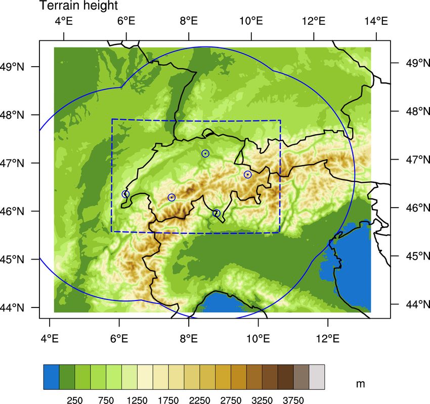
6496 T. H. Raupach et al.: Object-based analysis of simulated thunderstorms in Switzerland
ate output from numerical weather models (e.g. Done et al., approach provides a useful way to study future severe storm
2004; Davis et al., 2006a, b), including through the use of scenarios for Switzerland and other complex domains. The
storm tracking methods (Pinto et al., 2007; Caine et al., 2013; rest of this article is organised as follows: the data and meth-
Feng et al., 2018, 2021), and they are a useful way to statis- ods used are described in Sect. 2. Results of the simulation-
tically summarise and compare model outputs and observa- to-observation comparisons are shown in Sect. 3. Implica-
tions that may be otherwise difficult to compare (e.g. Gille- tions of the results are discussed and conclusions are drawn
land et al., 2010; Caine et al., 2013). Several methods for La- in Sect. 4.
grangian tracking of thunderstorms are available (e.g. Dixon
and Wiener, 1993; Hering et al., 2004; Feng et al., 2018;
Fridlind et al., 2019; Heikenfeld et al., 2019). In this arti- 2 Data and methods
cle we present a feasibility study to investigate the ability
of an existing radar-based thunderstorm tracker to perform In this section we introduce the data and methods used in
object-based analysis of simulated thunderstorms in the to- this work, starting with the study time period and location in
pographically complex region of Switzerland. Sect. 2.1. The reference dataset, which is used as the ground
Simulations were run using the Advanced Research truth for storm characterisation, is introduced in Sect. 2.2.
Weather Research and Forecasting (AR-WRF, version 4.0.1, The TITAN storm tracker is described in Sect. 2.3. The
hereafter WRF) weather model (Skamarock et al., 2019) at weather model we used to simulate thunderstorms is de-
convection-permitting grid spacing and high temporal reso- scribed in Sect. 2.4. The methods by which the storm prop-
lution for the month of May 2018. Thunderstorms were iden- erties for simulations are compared to the reference dataset
tified in the model output using the Thunderstorm Identifi- are explained in Sect. 2.5. Finally, optimisation of TITAN
cation, Tracking, Analysis and Nowcasting (TITAN; Dixon threshold parameters is described in Sect. 2.6.
and Wiener, 1993) algorithm (Git version lrose-cyclone-
20190801-167-g85b01e9a3) run on simulated radar reflec- 2.1 Study period and domain
tivity fields. In this paper the results are compared to a
database of thunderstorm observations for Switzerland (Nisi The study domain is centred over Switzerland, an area in
et al., 2018). These observations were made using the which complex topography affects precipitation processes
Swiss radar network and the MeteoSwiss-developed Thun- (e.g. Houze, 2012) and our ability to monitor them (e.g.
derstorms Radar Tracking (TRT; Hering et al., 2004, 2008) Germann et al., 2015; Speirs et al., 2017). Thunderstorms
algorithm. We consider the TRT algorithm results to be rep- (van Delden, 2001) and hailstorms (Houze et al., 1993;
resentative of the thunderstorm environment in Switzerland, Willemse, 1995; Punge and Kunz, 2016; Nisi et al., 2016;
and tested simulated thunderstorm results against this bench- Punge et al., 2017; Madonna et al., 2018) are a regular warm-
mark. season occurrences in Switzerland. The Swiss convective
TITAN has previously been applied to WRF output: Pinto season runs from April to September, with storms occur-
et al. (2007) used TITAN on WRF simulations and cor- ring primarily in the foothill regions north and south of the
responding radar observations in the southeastern United main Alpine range and in the Jura Mountains (Nisi et al.,
States of America and found that although the WRF simula- 2016, 2018). The most populous area in Switzerland – the
tions produced storms that initiated at similar times as the ob- Swiss Plateau, between the Jura and the Alps – is regularly
served storms, there were differences between the modelled affected by severe thunderstorms that can be long-lived and
and observed storm evolution and spatial coverage. More re- produce hail (Houze et al., 1993; Nisi et al., 2018). His-
cently, Caine et al. (2013) used TITAN to compare WRF out- torical cases include storms that inflicted significant dam-
put and radar data for tropical storms in northern Australia. age (e.g. Schmid et al., 1997, 2000; Peyraud, 2013; Trefalt
They showed the advantages of an object-based approach for et al., 2018). In Switzerland, severe storms are monitored
comparing models to observations and used it to determine primarily by a dual-polarisation radar network operated by
that WRF produced overly tall and small convective cells. MeteoSwiss (Germann et al., 2015). Switzerland’s climate
Our study is the first to apply such a technique to the complex is expected to be significantly affected by global warming
Alpine domain of Switzerland. A difference from previous (CH2018, 2018), but high uncertainty remains regarding the
studies is that we compare simulated thunderstorm properties likely future evolution of severe thunderstorms in Switzer-
to radar observations characterised by an independent thun- land (CH2018, 2018; Willemse, 1995).
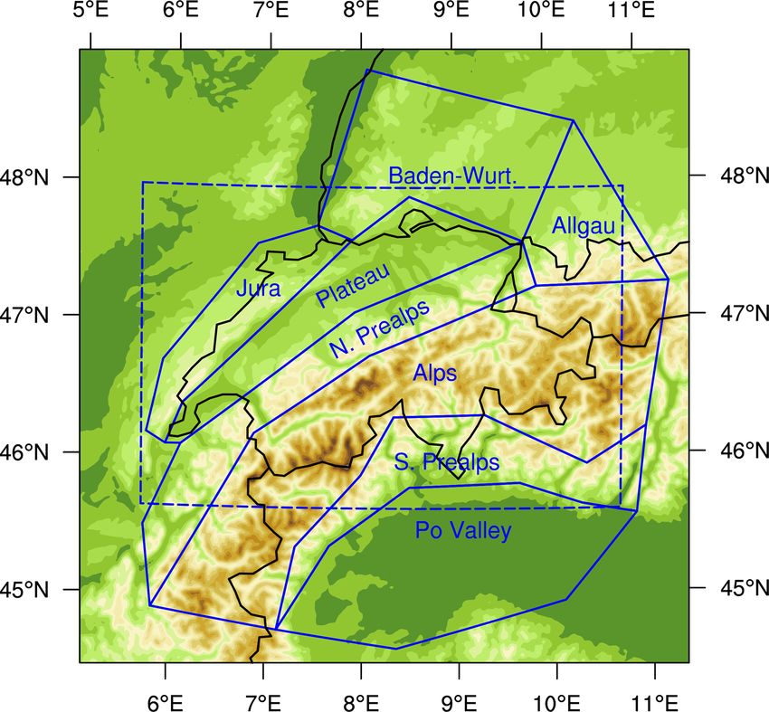
derstorm tracker designed specifically for the Swiss domain, Figures 1 and 2 show the geographical area of the study,
thus testing the ability of WRF and TITAN to characterise with the radar coverage area overlaid. The Alps run across
thunderstorms in the challenging Alpine environment. the centre of the simulation domain and split it into north-
In this work we aim to answer the question of whether ern and southern regions. Figure 3 shows the sub-domains
storm properties produced using WRF and TITAN are rea- used in this study; these correspond to geographical features
sonably representative of storms observed in Switzerland. If and are modified versions of the domains used by Nisi et al.
this question is answered in the positive, then this processing (2016). Table 1 lists the coordinates of the boundaries of the
Geosci. Model Dev., 14, 6495–6514, 2021 https://doi.org/10.5194/gmd-14-6495-2021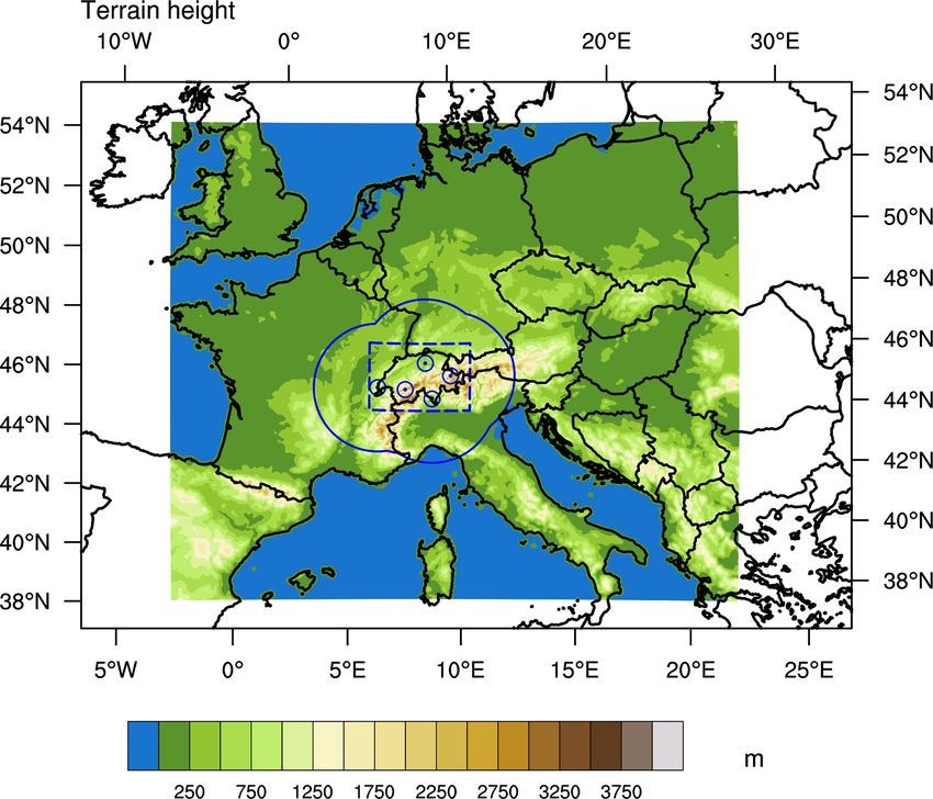
T. H. Raupach et al.: Object-based analysis of simulated thunderstorms in Switzerland                                                    6497

Table 1. Corner point coordinates for the study domain. E and N
are the Swiss coordinates (CH1903+/LV95) in the east and north di-
rections, respectively, while “long” and “lat” are the corresponding
longitude and latitude. L and R stand for left and right, respectively.

   Corner            E [m]        N [m]      Long [◦ ]      Lat [◦ ]
   Bottom L      2 464 500    1 056 000      5.70093     45.64222
   Top L         2 464 500    1 316 000      5.62372     47.98025
   Top R         2 854 500    1 316 000     10.84586     47.94466
   Bottom R      2 854 500    1 056 000     10.70117     45.60812

                                                                          Figure 2. As for Fig. 1, but for the inner (higher-resolution) nested
                                                                          WRF domain.

Figure 1. Terrain heights (above sea level) for points covered by
the WRF simulation outer domain. Black lines show national bor-
ders and coastlines. The locations of the five MeteoSwiss radars are
indicated with blue circled points, and the solid blue line shows the
approximate radar domain. The dashed blue line shows the study
domain. Storms with centre points outside the study domain are not
considered in this study. Elevations below 0.001 m are plotted in
blue. Plot produced using the NCAR Command Language (NCL)
version 6.6.2.

study domain, which was chosen to be well covered by both
the radar data and simulations.
   The study period was May 2018. In Switzerland, the 2018
                                                                          Figure 3. Sub-domains used in this study (solid blue lines). Terrain
convective season was characterised by lower than average                 elevation and national borders are shown as in Fig. 1. “N. Prealps”
overall rainfall (MétéoSuisse, 2018c) but high levels of con-             stands for northern Prealps, “S. Prealps” stands for southern Pre-
vective activity in late May and early June (MétéoSuisse,                 alps, and “Baden-Wurt.” stands for Baden-Württemberg. The study
2018b, a). In May, thunderstorms occurred in Switzerland on               domain is shown by the dashed blue line. Plot produced using NCL
days 6–9 and 11–13 of the month and then almost daily from                version 6.6.2.
the 15th until the end of the month (MétéoSuisse, 2018b).
22 May saw thunderstorms across the Central Plateau with
a 30-year daily rain amount (73.2 mm) at Belp, and on 30                  2.2   Reference thunderstorm dataset
and 31 May there were extensive hailstorms over the Swiss
Plateau that caused local flooding (MétéoSuisse, 2018b).                  The reference data for thunderstorms in Switzerland are
Hail was reported in Switzerland on, 7, 8, 15, 21, 30, and                found in a database of thunderstorm tracking results com-
31 May (Sturmarchiv Schweiz, 2019).                                       piled by MeteoSwiss. MeteoSwiss operates five C-band,
                                                                          dual-polarisation, Doppler weather radars in a network de-

https://doi.org/10.5194/gmd-14-6495-2021                                                      Geosci. Model Dev., 14, 6495–6514, 2021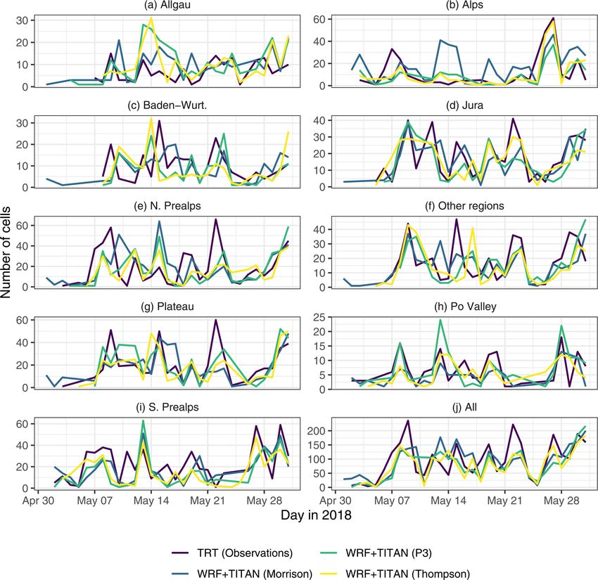
6498                               T. H. Raupach et al.: Object-based analysis of simulated thunderstorms in Switzerland

signed for high performance despite the challenges posed           2.3   The TITAN storm tracker
by the mountainous terrain of Switzerland (Germann et al.,
2015). The resulting radar products are at high spatial and        TITAN is a radar-based storm cell tracker that uses thresh-
temporal resolution, with 20 elevation sweeps conducted ev-        olds on 3D Cartesian fields of radar reflectivity to define
ery 5 min (Germann et al., 2015). The locations and approx-        contiguous storm areas, for which statistical properties are
imate horizontal coverage area of the radar network are plot-      calculated (Dixon and Wiener, 1993). Matching of storms
ted in Figs. 1 and 2. The reference dataset we use in this study   between time steps is performed using an optimisation algo-
contains results from the TRT algorithm that were compiled         rithm that expects matched storms to have similar volumes
into a database of storm cells and their associated properties     and prioritises small separation distance (Dixon and Wiener,
(as in Nisi et al., 2018, but including data for 2018 and using    1993). TITAN has been used operationally (e.g. Bally, 2004)
all Swiss radars).                                                 and in an object-based study of hailstorm properties (Foris
   TRT was developed specifically to deal with the challeng-       et al., 2006). We chose to use TITAN because of its free avail-
ing topography of the Alpine region: it takes advantage of the     ability and long history of operational use; we note that other
high spatial and temporal resolution of the Swiss radar net-       tracking methods are also available (e.g. Fridlind et al., 2019;
work (Nisi et al., 2016). TRT identifies thunderstorms in a        Heikenfeld et al., 2019).
two-dimensional Cartesian multiple-radar “max echo” com-              TITAN (Dixon and Wiener, 1993; TITAN system within
posite product, which is composed of the maximum radar             LROSE, 2019) was downloaded and compiled from the Li-
reflectivity recorded in each vertical column (Nisi et al.,        dar Radar Open Source Software Environment (LROSE).
2014). TRT uses an adaptive thresholding scheme proposed           TITAN uses specialised binary formats for both input and
by Crane (1979) that requires a fixed minimum detection            output. As input, TITAN requires data in Meteorological
threshold Zmin [dBZ], a fixed minimum reflectivity “depth”         Data Volume (MDV) format with radar reflectivity fields
Zdepth [dBZ], and an adaptive threshold Zthresh [dBZ]. On a        in 3D Cartesian gridded coordinates (Dixon and Wiener,
two-dimensional map of max echo radar reflectivity, a cell         1993). We used an adapted version of the TITAN tool
is defined as a closed contour at Zthresh [dBZ] around a           NcGeneric2Mdv to convert input files to MDV format.
maximum reflectivity of Zpeak [dBZ]. Zthresh is adapted for        The outputs of the tracking process are “storm” files, in
each cell to be the minimum value for which Zthresh ≥ Zmin         which the tracking results are stored in binary format. To ex-
and for which the cell contains a single closed contour at         tract storm properties from the storm files we used an adapted
Zpeak − Zdepth dBZ (Crane, 1979; Hering et al., 2004). In the      version of the TITAN Storms2Xml2 tool. The TITAN pro-
case of TRT, Zmin is 36 dBZ and Zdepth is 6 dBZ, and a fur-        cessing flowchart for simulation data is shown in Fig. 4.
ther constraint on cell area is applied: for a thunderstorm to        For this study we ran TITAN in dual-thresholding mode
be detected by TRT it must contain a connected area of suf-        with auto-restart disabled. In dual-thresholding mode, storms
ficient size with radar reflectivity values at 36 dBZ or higher    are identified in two steps. First, regions of reflectivity above
and at least one pixel with a reflectivity of at least 42 dBZ      a lower threshold are identified. Then, within these regions,
(Hering et al., 2004). The area threshold used in these obser-     areas with reflectivities greater than a sub-region reflectivity
vations was 13 km2 (Alessandro Hering, personal commu-             threshold are identified, tested for size, and “grown” out into
nication, 2020). TRT uses geographical overlapping of cells        the original lower-threshold region (Dixon and Seed, 2014).
for matching between time steps (Hering et al., 2004, 2008).       Threshold choice is discussed in Sect. 2.6.
Several cell properties are then computed by TRT from the
3D radar data, as well as satellite and lightning data, inside     2.4   WRF weather model
the detected footprint of each cell. A cell severity ranking
product is included.                                               WRF is a weather model used for both research and op-
   TRT is well tested and established as a reference dataset. It   erational numerical weather prediction (NWP) (Skamarock
has been in operational use at MeteoSwiss since 2003 (Her-         et al., 2019; Powers et al., 2017). When run at sufficiently
ing et al., 2008) and formed part of a successful forecast         high spatial resolution, it can explicitly resolve convection.
demonstration project in the Alpine region (Rotach et al.,         What constitutes a sufficient resolution depends on the appli-
2009). TRT was used to produce a 15-year, Lagrangian-              cation: model grid spacings finer than 1 km are optimal for
perspective hail climatology for Switzerland (Nisi et al.,         resolving all convective processes, while proper resolution
2018), as well as to study hailstorm initiation with cold fronts   of turbulent processes requires a grid spacing of the order of
(Schemm et al., 2016). In this study we use TRT results for        100 m (e.g. Bryan et al., 2003; Bryan and Morrison, 2012).
the study period as the reference dataset. TRT code is not         However, grid spacings up to 4 km provide enough detail to
freely available, so in this study we use a generalised open-      explicitly resolve basic cumulous cloud structures (e.g. Weis-
source storm tracker and compare its results to the state-of-      man et al., 1997; Done et al., 2004; Kain et al., 2006; Chevu-
the-art closed-source results of TRT.                              turi et al., 2015). In this work we ran WRF with 50 vertical
                                                                   levels on a regional rotated grid with an average horizontal
                                                                   resolution of about 1.5 × 1.5 km2 . A nested domain struc-

Geosci. Model Dev., 14, 6495–6514, 2021                                             https://doi.org/10.5194/gmd-14-6495-2021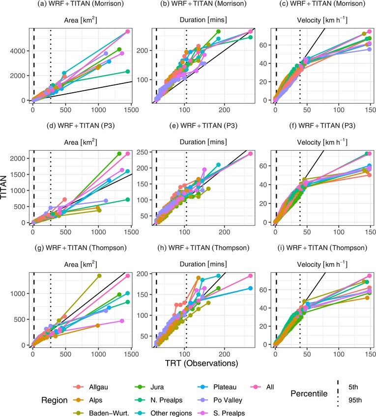
T. H. Raupach et al.: Object-based analysis of simulated thunderstorms in Switzerland                                           6499

Figure 4. The processing flowchart used in this study for WRF data. Shown are input data (blue) processing steps (green) and analyses
(yellow). Nc2Mdv is a modified version of the TITAN tool NcGeneric2Mdv, and stormStats is a modified version of the TITAN tool
Storms2Xml2.

ture was used with a larger external domain at an average of         2.5   Comparing storm properties
about 4.6 × 4.6 km2 resolution. The two domains are shown
in Figs. 1 and 2, respectively.                                      Before comparisons of tracking results were made, TRT and
   We used WRF version 4.0.1 (Wang et al., 2018). HAIL-              TITAN cell detections with centre points outside the study
CAST (Brimelow et al., 2002; Adams-Selin and Ziegler,                domain (see Fig. 2) were discarded. Cells that were truncated
2016) was used to calculate maximum hail sizes. We tested            by this operation had their durations shortened to the duration
three different WRF microphysics schemes: the Predicted              for which they stayed within the region of interest. Likewise,
Particle Property (P3) scheme (Morrison and Milbrandt,               cells that were split into multiple parts by the spatial subset-
2015), the Morrison scheme (Morrison et al., 2009), and              ting operation were updated so that their parts were counted
the Thompson scheme (Thompson et al., 2008). The other               as separate storm cells.
schemes used in the model are shown in Table 2. The bound-              Thunderstorms often split into multiple parts or merge
ary data used were European Centre for Medium-Range                  from multiple parts into single cells. TITAN and TRT handle
Weather Forecasts (ECMWF) operational analyses from the              the labelling of these storms differently. TITAN data contain
Integrated Forecasting System (IFS) cycle 43r3 (ECMWF,               a “storm ID” that is maintained through splits and merges and
2017; Buizza et al., 2017). Radar reflectivity was calcu-            a “track ID”, which refers to a unique length of storm track
lated by WRF, with the option do_radar_ref enabled                   with no splits or merges. TRT data contain flags indicating
to instruct WRF to calculate reflectivity using microphysics-        when splits and merges have occurred, and the most intense
scheme-specific parameters (Wang et al., 2018). The simula-          storm part keeps the same identifier afterwards. Due to these
tions covered May 2018 at 5 min resolution.                          labelling differences, in this paper we take a simplified ap-
   Storm tracking was run on the WRF output variable                 proach and refer to a “cell” as a region of high radar reflectiv-
REFL_10CM, which contained estimated 10 cm wavelength                ity that exists for at least 30 min with no splitting or merging
(S-band) radar reflectivity in decibels relative to reflectivity     events. When a split occurs, the parent cell ends and multi-
(dBZ) as produced by the WRF microphysics scheme. The                ple new (child) cells are created, and when a merge occurs
WRF data were treated using an NCAR command language                 multiple cells end and a new (merged) cell is created. In this
(NCL, version 6.4.0, NCL6.4) script to regrid the data to a          way we lose information on the overall length of one storm
Cartesian grid stored in NetCDF format. The files were first         system, but we can compare cell properties easily and fairly.
regridded horizontally by dividing the WRF domain into a             A “track” is the path over which a cell moves. A “cell de-
grid with the same number of points and extents of latitude–         tection” refers to a region of high reflectivity at one moment
longitude values as the input fields, but with the points as         in time. Some storm properties (area, movement direction)
evenly spaced as possible on each axis. The regridding was           are defined for each cell detection, while some (duration) are
performed using bilinear interpolation provided by the Earth         defined for each cell.
System Modeling Framework (ESMF, version 8.0.0; Val-                    The TRT results are taken as the reference dataset, and
cke et al., 2012) through NCL. The output grid had a res-            TITAN results were compared to the TRT database to anal-
olution of approximately 0.0141◦ latitude by 0.0211◦ lon-            yse the performance of the TITAN approach. The compari-
gitude. This grid was then interpolated vertically using the         son measures used were defined as follows: for a given storm
NCL wrf_user_vert_interp function to grid points                     property P , let Pi,TITAN be the ith value of the property given
from 1 to 15 km above sea level at 0.5 km resolution. These          by the TITAN approach and let Pi,TRT be the corresponding
heights were geopotential heights above sea level; the small         ith reference value of the property in the TRT database (i
differences between geopotential and geometric heights are           refers to an index shared by both datasets, such as simulation
ignored in this study. Interpolation of radar reflectivities was     day). The difference between the two results is given by
performed using dBZ values. The regridded WRF files were
                                                                     Di = Pi,TITAN − Pi,TRT .                                     (1)
converted to MDV format for use with TITAN.
                                                                     The bias of the TITAN approach is hDi, where the angular
                                                                     brackets signify the mean of all differences. The root mean

https://doi.org/10.5194/gmd-14-6495-2021                                               Geosci. Model Dev., 14, 6495–6514, 2021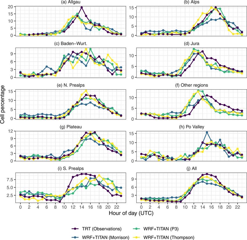
6500                                 T. H. Raupach et al.: Object-based analysis of simulated thunderstorms in Switzerland

Table 2. Schemes used in the WRF model in this study.

                          Configuration option           Scheme used
                          Boundary layer scheme          Yonsei University (Hong et al., 2006)
                          Cumulus parameterisation       None (explicit convection)
                          Shortwave radiation scheme     Dudhia (Dudhia, 1989)
                          Longwave radiation scheme      RRTM (Mlawer et al., 1997)
                          Land surface scheme            Noah (Chen and Dudhia, 2001)
                          Surface layer model            Revised MM5 Monin–Obukhov (Jiménez et al., 2012)
                          Hail model                     HAILCAST (Adams-Selin and Ziegler, 2016)

                           p
squared error (RMSE) is        hD 2 i. The relative error is given     tested values from low_dbz_threshold plus 4 dBZ
as a percentage by                                                     to low_dbz_threshold plus 12 dBZ in 1 dBZ incre-
                                                                       ments; and (3) the volume threshold for cell detection
       100Di
Ri =          .                                               (2)      min_storm_size, with tested values of 25, 50, and
       Pi,TRT                                                          75 km3 .
The mean relative bias (RB, hRi), the median relative bias                TITAN was run on WRF output for the test days with all
(MRE, median of R), and the interquartile range of relative            243 tested combinations of the three thresholds. The results
bias (RE IQR, 75th percentile minus 25th percentile of R)              for each run were compared to TRT results for those days.
are used to measure relative differences. The squared Pearson          The “best” parameter set was non-trivial to select and de-
correlation coefficient (r 2 ) is used to show the co-fluctuation      pended on the performance metrics used. We chose an ap-
of PTITAN and PTRT . The relative error is only defined when           proach that emphasised low bias and co-fluctuation in the
Pi,TRT is non-zero; accordingly, RB, MRE, and RE IQR in-               simulated and observed number of cells per hour and a good
clude only data points for which Pi,TRT 6 = 0, whereas bias,           match for cell area. To choose the “winning” parameter set
RMSE, and r 2 include such points. Days on which no tech-              we used the absolute value of median relative bias as a score.
nique identified cells are not counted in the statistics.              This score was applied to comparisons of daily median cell
                                                                       area and per-time-step number of cells. We first subset based
2.6    Optimisation of TITAN thresholds                                on the number of cells per hour by taking all test runs with
                                                                       scores less than the 10th percentile of all scores. We then sub-
Radar reflectivities simulated in WRF at S-band are not ex-            set based on daily median cell area by again taking scores
pected to match the measured radar reflectivities at C-band            less than the 10th percentile of all such scores. Of the few
that were used by TRT, so we did not attempt to make TITAN             remaining tested combinations, we chose the configuration
use exactly the same thresholds as TRT. Furthermore, the               with the best squared correlation coefficient value for the
TRT detection works on two-dimensional fields and thresh-              simulated and observed per-time-step number of cells. The
olds on cell area, whereas TITAN uses three-dimensional                resulting thresholds used for TITAN tracking in this study
fields and thresholds on cell volume. Our simulation setups            are shown in Table 3. Reports showing details of the thresh-
differed only in the microphysics scheme used, but since the           old testing are archived (Raupach et al., 2021d).
calculation of radar reflectivities can be affected by the mi-            Other parameters in the dual-thresholding scheme were
crophysics scheme as well as the assumed radar frequency,              held fixed for all model runs. These parameters were the min-
optimum thresholds were expected to differ between simula-             imum area required for each sub-part in the dual-thresholding
tion sets.                                                             approach (min_area_each_part), which was set to
   We chose to optimise three TITAN thresholds by find-                16 km2 , the fraction of the lower-reflectivity storm region
ing the values that provided the best match between TI-                that must be covered by the sum of all higher-reflectivity sub-
TAN+WRF (simulation) output and TRT results (obser-                    regions (min_fraction_all_parts), set to 0.10, and
vations) for 29 and 30 May 2018, 2 d over which thou-                  the minimum proportion of the large area that each sub-area
sands of storm detections were made across the do-                     must exceed (min_fraction_each_part), set to 0.005.
main. The optimised thresholds were then used for val-                 These last two area thresholds are those listed in the default
idation of the technique with the whole dataset for                    TITAN parameters as appropriate for strong convection and
May 2018. The three thresholds tested were the fol-                    squall lines in South Africa1 .
lowing: (1) the reflectivity threshold for cell detection
(low_dbz_threshold in the TITAN parameter file),
with tested values from 34 to 42 dBZ in 1 dBZ incre-                       1 Stated in the TITAN paramdef.TITAN file at
ments; (2) the reflectivity threshold for dual threshold-              https://github.com/NCAR/lrose-core/blob/master/codebase/apps/
ing (dbz_threshold under dual_threshold), with                         titan/src/Titan/paramdef.Titan (last access: 23 December 2019).

Geosci. Model Dev., 14, 6495–6514, 2021                                                https://doi.org/10.5194/gmd-14-6495-2021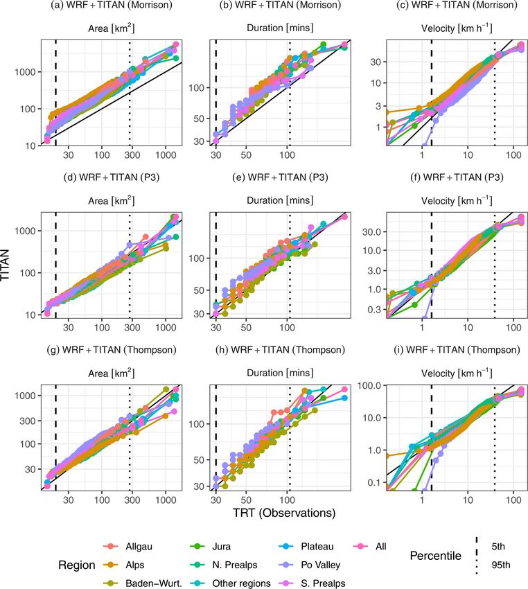
T. H. Raupach et al.: Object-based analysis of simulated thunderstorms in Switzerland                                      6501

Table 3. The threshold values used in each application of TI-      3.1   Spatial and temporal cell occurrences
TAN. Other thresholds were left at default values. These thresh-
olds are for the basic detection threshold (Z threshold, the       Figure 5 shows a comparison of the number of storm detec-
low_dbz_threshold parameter), the dual-thresholding sub-           tions (cell–time combinations) per 10 × 10 km2 raster grid
region threshold (sub-region Z threshold, dual_threshold’s         point to show the “hotspots” of storm activity during the
dbz_threshold parameter), the minimum allowed storm vol-
                                                                   month of May 2018 in both the simulations and observations.
ume (min. volume, the min_storm_size parameter), and the
minimum area for sub-parts (min. sub-area, dual_threshold’s
                                                                   The figure shows broadly similar spatial layouts between ob-
min_area_each_part parameter).                                     servations and simulations. In particular, the observations
                                                                   and all simulations show regions of increased storm occur-
                   Z         Min.       Min.     Sub-region Z      rence over the northern flanks of the Jura Mountains that run
               threshold   sub-area   volume       threshold       along the border of Switzerland and France, southwestern
                 [dBZ]      [km2 ]     [km3 ]        [dBZ]         Germany, the southern Swiss Plateau and northern Prealps,
                                                                   and northern Italy to the east of Ticino (the part of Switzer-
    Morrison      42          16         50           54           land that extends into the southern Prealps region shown in
    P3            39          16         50           47
                                                                   Fig. 3). The simulated storm hotspots over the Jura are to the
    Thompson      40          16         75           47
                                                                   north of the observed Jura hotspot. Notably, the simulations
                                                                   all underestimate the concentration of storm detections in Ti-
                                                                   cino observed by radar. The simulations all reproduce the
3    Results                                                       minima of storm activity that traces the main Alpine range; in
                                                                   this regard, the P3 and Thompson schemes produce more re-
In this section, storm properties found using TITAN with
                                                                   alistic maps than the Morrison scheme. Overall, the approach
WRF simulation output are compared to those found using
                                                                   of using TITAN with WRF output is able to broadly repro-
TRT with radar data to test whether TITAN applied to WRF
                                                                   duce the observed locations of cell detection maxima.
simulations can produce representative statistics on thunder-
                                                                       Figure 6 shows the number of cells detected by each tech-
storms in Switzerland. TITAN was run over the WRF simu-
                                                                   nique on each day of May 2018. Table 5 shows statistics to
lation outputs, and TRT results were subset to the same pe-
                                                                   compare the number of cells per day between the simula-
riod of time. Both sets of results were subset to the study do-
                                                                   tions and observations. Because the simulations and obser-
main shown by the dashed line in Figs. 1 and 2. During sub-
                                                                   vations are independent and the simulations are forced only
setting of the TITAN (TRT) results, including all tested mi-
                                                                   by lower-resolution boundary conditions, we do not neces-
crophysics scheme setups, subsetting caused splits in 0.78 %
                                                                   sarily expect an exact match in cell occurrence time series.
(0.64 %) of cells. After subsetting, 37.8 % (52.4 %) of the
                                                                   The simulated number of cells detected per day shows mag-
recorded cells were discarded because their track duration
                                                                   nitudes similar to the observations, with exceptions in All-
was less than 30 min. The resulting cell descriptions from
                                                                   gäu, the Alps for the Morrison scheme, and the Po Valley
TITAN sometimes contained spatial overlaps; 23 % of cells
                                                                   for the P3 scheme, where more cells were detected in the
were affected by overlaps, but the areas affected were small,
                                                                   simulations. In terms of median relative bias, the best per-
with only 3 % of all cell points overlapping. Of the TRT
                                                                   region performance was with the Thompson scheme in the
cells remaining after subsetting, 30 (0.06 %) were removed
                                                                   Alps region (−2 %), and the best performance for all re-
from this analysis because no cell velocity information was
                                                                   gions combined was with the Morrison scheme (−13 %). The
recorded.
                                                                   worst overall match was with the P3 scheme (−20 %). The
   Table 4 shows a comparison of the number of detections
                                                                   worst per-region median relative bias was with the Morrison
(here defined as unique storm–time combinations) and storm
                                                                   scheme in the Alps region (78 %). The greatest co-fluctuation
cells captured by each technique. When each microphysics
                                                                   (r 2 value) in a single region was shown by the Thompson
scheme was compared to the reference TRT dataset, TITAN
                                                                   setup in the Alps region (0.74) and overall by the Thompson
produced 15 % more detections for the Morrison scheme,
                                                                   scheme (0.56). That positive correlations exist for cells per
9 % fewer detections for the P3 scheme, and 15 % fewer
                                                                   day shows that the WRF model is able to use these bound-
detections for the Thompson scheme. TITAN produced 4 %
                                                                   ary conditions to produce thunderstorm cells on storm-prone
fewer cells for the Morrison scheme, 19 % fewer cells for the
                                                                   days.
P3 scheme, and 19 % fewer cells for the Thompson scheme
                                                                       To investigate any systematic timing differences and to
than were in the TRT dataset. In the rest of this section,
                                                                   look at the diurnal cycle of the thunderstorms, we calculated
we show detailed comparisons with sub-regions identified
                                                                   the percentage of cells that appeared in each hour of the day
as shown in Fig. 3. The thunderstorm properties are divided
                                                                   for each simulation and for the observations. These results
into four categories: spatial and temporal cell occurrences
                                                                   are shown by region in Fig. 7. In all regions, the afternoon
(Sect. 3.1), cell movement properties (Sect. 3.2), hail prop-
                                                                   peak in thunderstorm activity is well reproduced by the sim-
erties (Sect. 3.3), and storm life cycle properties (Sect. 3.4).
                                                                   ulations, although the exact timings differ from the observa-
                                                                   tions in some regions. There is a tendency for the Morrison

https://doi.org/10.5194/gmd-14-6495-2021                                             Geosci. Model Dev., 14, 6495–6514, 2021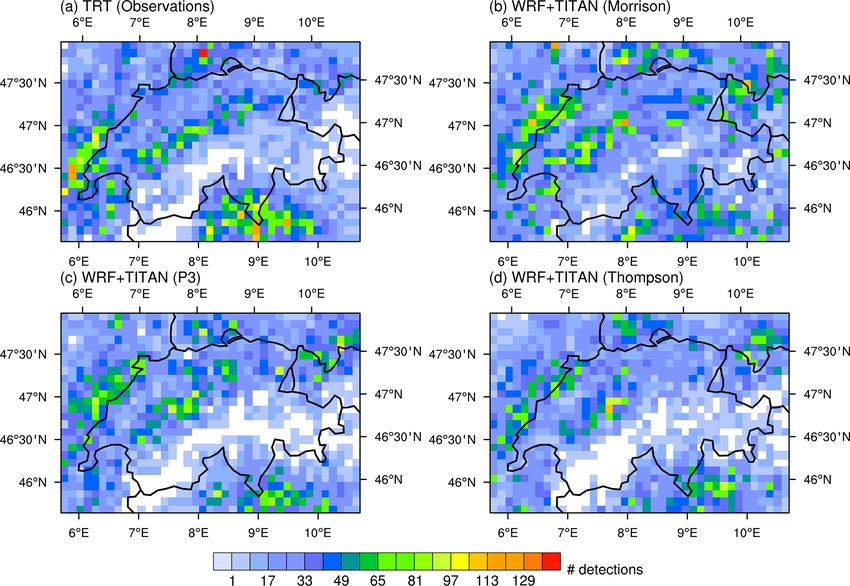
6502                                 T. H. Raupach et al.: Object-based analysis of simulated thunderstorms in Switzerland

Table 4. Summary information for each dataset, showing the number of cell detections (cell–time combinations), number of cells, and first
and last cell detection times.

                 Method                          No. detections   No. cells    First cell (UTC)      Last cell (UTC)
                 WRF + TITAN (Morrison)                 29 865        2708     1 May 2018, 00:00     31 May 2018, 23:55
                 WRF + TITAN (P3)                       23 696        2292     2 May 2018, 22:35     31 May 2018, 23:55
                 WRF + TITAN (Thompson)                 21 974        2301     3 May 2018, 04:40     31 May 2018, 23:35
                 TRT (observations)                     25 921        2831     2 May 2018, 19:10     31 May 2018, 23:55

Figure 5. The overall number of cell detections (cell–time combinations) in each 10 × 10 km2 grid point, for May 2018, for observations (a)
and simulations with three different microphysics schemes (b–d). Plot produced using NCL version 6.6.2.

and P3 simulations to produce more cells during the night-              south of the main Alpine chain (Nisi et al., 2016, and ref-
time than are observed, and this continues into the morning             erences within).
for the Morrison scheme. For all data, the peak time for cell
occurrence in the Thompson simulations matches the peak
time in the observations, while the peak in the Morrison set            3.2   Cell movement properties
is 1 h earlier, and there are peaks in the P3 scheme both 1 h
earlier and 1 h later than the observed peak at 15:00 UTC.              The use of object-based analysis means we can compare ag-
There is an interesting pattern in the results in which simu-           gregate storm properties such as movement speed, direction,
lated storms tend to appear earlier than the observed storms            intensity, or cell lifetime. Figure 8 shows a comparison of the
in the north and northwest (Jura, Allgäu, other regions), at            directions in which detected cells were moving at each obser-
about the same time as the observations in central Switzer-             vation point. Although there are some differences in the pro-
land (Alps, N. Prealps, plateau), and later than the observa-           portions between TRT and TITAN, it is notable that the sim-
tions in the southern Prealps. The results for the Po Valley            ulations are able to reproduce the differences in advection di-
match the observations well. Earlier storms in the north and            rection observed between different regions. For example, the
later storms in the south have been shown in previous radar-            TRT observations show that storms moved mostly in a north
based climatologies (Nisi et al., 2016), but here this effect           and northwest direction in the Po Valley and in a southwest
is more extreme in the simulations than in the observations.            direction on the Swiss Plateau. The simulations reproduce
The north-to-south differences are possibly due to different            these differences. Again, the region of Allgäu shows notable
handling of convective initiation mechanisms in the weather             differences between observations and simulations. Table 6
model. There are known differences in storm initiation be-              shows the mean direction of all cells by region and dataset.
tween northern regions of Switzerland and regions to the                The simulation set that produced the best match to observa-

Geosci. Model Dev., 14, 6495–6514, 2021                                                  https://doi.org/10.5194/gmd-14-6495-2021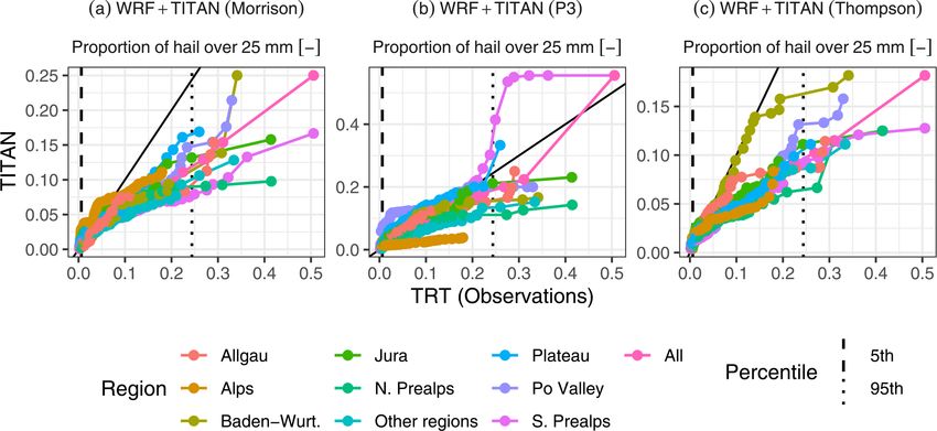
T. H. Raupach et al.: Object-based analysis of simulated thunderstorms in Switzerland                                                    6503

Table 5. Performance statistics on cells detected per day per region, with TRT (observations) taken as the reference. Statistics shown are bias
[d−1 ], root mean squared error (RMSE) [d−1 ], relative bias (RB) [%], median relative error (MRE) [%], interquartile range of relative error
(RE IQR) [% points], and squared Pearson correlation (r 2 ) [–].

                                                                       Bias    RMSE        RB    MRE      RB IQR        r2
                   WRF + TITAN (Morrison)           Allgäu             2.8        7.7     126      10          142    0.04
                                                    Alps               8.1       16.8     394      78          448    0.20
                                                    Baden-Wurt.       −0.3        8.4      34     −15          178    0.07
                                                    Jura              −1.5        9.5      26     −10          132    0.45
                                                    N. Prealps        −1.0       19.1     110     −15          145    0.13
                                                    Other regions     −1.4       11.3      28     −16           91    0.38
                                                    Plateau           −0.8       14.1      70     −10           81    0.30
                                                    Po Valley         −1.7        4.7      36     −33           50    0.28
                                                    S. Prealps        −4.4       15.1      51     −31          129    0.28
                                                    All               −3.7       52.5      44     −13          109    0.41
                   WRF + TITAN (P3)                 Allgäu             3.0        8.6     115      12          212    0.11
                                                    Alps              −2.5       10.5      47     −15          190    0.57
                                                    Baden-Wurt.       −1.8        9.4      21     −33           90    0.03
                                                    Jura              −3.3        9.6     −4      −16           64    0.50
                                                    N. Prealps        −4.1       17.6     −7       −9          106    0.24
                                                    Other regions     −2.1       13.6       5     −27           93    0.23
                                                    Plateau           −0.9       13.5     −7      −12           73    0.40
                                                    Po Valley         −0.2        4.8      49     −29           97    0.49
                                                    S. Prealps        −7.9       15.6     −7      −44           68    0.39
                                                    All              −18.3       49.2     −6      −20           71    0.52
                   WRF + TITAN (Thompson)           Allgäu             2.3        8.3      81      30          188    0.09
                                                    Alps              −0.3        7.7      37      −2           75    0.74
                                                    Baden-Wurt.       −1.3       10.9      48     −40           90    0.00
                                                    Jura              −3.2        9.8      18     −26           94    0.45
                                                    N. Prealps        −5.8       16.0      −4     −33          102    0.31
                                                    Other regions     −3.3       14.3      16     −20          104    0.20
                                                    Plateau           −3.2       14.1       8     −44           81    0.37
                                                    Po Valley         −1.5        5.0      29     −50           52    0.21
                                                    S. Prealps        −6.6       13.3     −11     −27           90    0.51
                                                    All              −18.2       46.8      −1     −19           57    0.56

Table 6. Mean advection directions by region.

                                                                        Mean angle (◦ )
        Region            TRT (observations)     WRF + TITAN (Morrison)         WRF + TITAN (P3)        WRF + TITAN (Thompson)
        Allgäu                            314                             17                     319                              323
        Alps                              349                            358                     334                              359
        Baden-Wurt.                       246                            310                     287                              312
        Jura                              322                            344                     350                              357
        N. Prealps                        301                             24                     348                              352
        Other regions                     269                            292                     309                              284
        Plateau                           261                            316                     290                              306
        Po Valley                         322                            305                     327                              348
        S. Prealps                        333                            340                     344                              338
        All                               295                            340                     327                              332

https://doi.org/10.5194/gmd-14-6495-2021                                                      Geosci. Model Dev., 14, 6495–6514, 2021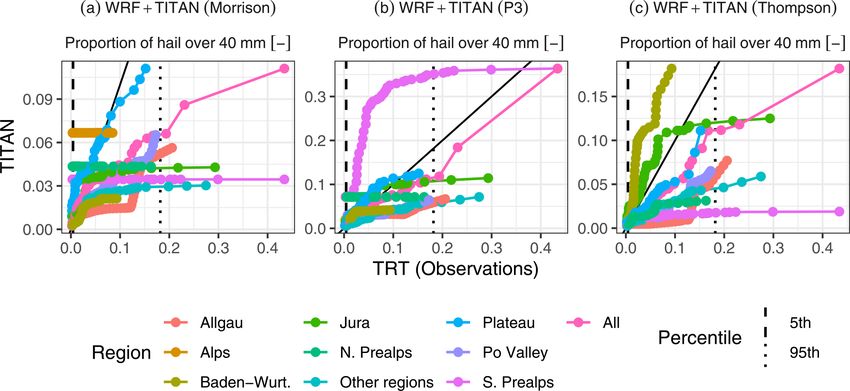
6504                                T. H. Raupach et al.: Object-based analysis of simulated thunderstorms in Switzerland

Figure 6. The number of cells detected per day in May 2018 for observations and simulated outputs per region (regions shown in Fig. 3).

tions differed by region, but the P3 scheme produced the best          unlikely to be caused by the microphysics scheme as such,
match in more regions than the other simulation sets.                  but rather by the thresholds that result from the optimisation
   Figure 9 shows quantile-to-quantile (QQ) comparisons of             process described in Sect. 2.6.
three other properties: cell detection areas, cell detection ve-
locities, and cell durations. We consider very high velocities         3.3   Hail properties
(> 80 km h−1 ) to be unrealistic artefacts of the tracking al-
gorithms; for both TRT and TITAN + WRF results less than
                                                                       In this section we compare radar-based observations of hail
0.5 % of cell detections had such velocities. We note again
                                                                       properties to those estimated by the WRF model and HAIL-
that these durations are the durations of cells as defined here,
                                                                       CAST. The object-based technique we test here may be par-
meaning that they are interrupted by storm splits and merges.
                                                                       ticularly useful for studying the effects of climate change
The QQ plots map observed quantiles of these properties to
                                                                       on hail, for which high uncertainty remains (e.g. Raupach
simulated quantiles over all detected cells. If the simulated
                                                                       et al., 2021b). In each dataset we compare the proportion
distributions match the observed distributions, the lines fol-
                                                                       of storm cell pixels that were estimated to contain severe
low the diagonal (solid black) line on the QQ plot. The plot
                                                                       (greater than 2.5 cm) and very large (greater than 4 cm) hail.
shows that the simulated distributions broadly agree with ob-
                                                                       In the observations from TRT, the maximum hail size was
served distributions for velocity in all simulations and for
                                                                       estimated using the radar-based maximum expected severe
area and duration for the P3 and Thompson microphysics
                                                                       hail size (MESHS; implementation described in Nisi et al.,
scheme setups. For the simulations run with Morrison mi-
                                                                       2016). In the WRF output, we used the HAILCAST vari-
crophysics, the plot shows that the detected cell areas were
                                                                       able HAILCAST_DIAM_MAX to calculate the proportions of
larger than the observed cells, and the simulated cells lasted
                                                                       TITAN-identified cell pixels with hail over 2.5 and 4 cm, re-
for longer durations than the observed cells. Cell area and
                                                                       spectively. We note that the two techniques used to estimate
duration are most affected by the choice of thresholds used
                                                                       maximum hail size are very different from each other and are
in the TITAN tracker, which means that these differences are
                                                                       therefore not strictly directly comparable; they are used here

Geosci. Model Dev., 14, 6495–6514, 2021                                                  https://doi.org/10.5194/gmd-14-6495-2021
T. H. Raupach et al.: Object-based analysis of simulated thunderstorms in Switzerland 6505
Figure 7. Percentages of cells that were active in each hour of the day per region in May 2018, with observations compared to simulation
outputs. Values are the percentage of all unique cell–hour combinations that occurred in each individual hour of the day so that values for
each curve sum to 100.
Table 7. Proportions of total cell detections that contained hail with cell detections with hail over 2.5 cm. The relative errors in
estimated diameter greater than 25 mm or 40 mm for observations these proportions were smaller for 2.5 cm hail than for 4 cm
and simulation outputs. hail, implying that the WRF and HAILCAST simulations
more severely underestimated the number of cells contain-
Proportion of cell detections ing very large hail than severe hail. Figures 10 and 11 show
with hail over quantile-to-quantile plots to compare the proportions of cell
25 mm [%] 40 mm [%] pixels, for cell detections for which the proportion was non-
zero, that contained hail with maximum estimated size over
TRT (observations) 3.2 1.3
2.5 cm and over 4 cm, respectively. The WRF results show an
WRF + TITAN (Morrison) 1.5 0.2
WRF + TITAN (P3) 1.6 0.5
underestimation of the cell area covered by severe and large
WRF + TITAN (Thompson) 2.5 0.4 hail compared to the TRT observations.
3.4 Cell life cycles
as the available approximations of observed and simulated In this section we consider cell life cycles – the evolution
hail size. of the strength of storm cells over their durations. Since in
Table 7 shows the proportions of all cell detections that this work splits and merges of storms interrupt storm du-
contained severe hail. In general, the observations contained rations, in this section we consider only the 43 % of cells
more severe hail than the simulations. All WRF setups un- that contained no splits or merges so that their durations are
derestimated the proportion of cell detections containing se- well defined. Figure 12 shows the number of such cells by
vere hail. The WRF setup using the Thompson microphysics cell duration. There are very few cells with a duration over
scheme produced the closest match to the TRT proportion of 100 min, meaning little emphasis should be placed on aggre-
https://doi.org/10.5194/gmd-14-6495-2021 Geosci. Model Dev., 14, 6495–6514, 20216506 T. H. Raupach et al.: Object-based analysis of simulated thunderstorms in Switzerland Figure 8. Comparison of tracked cell directions by TITAN (on WRF data) and TRT (on radar observations). Shown are the percentages of times cells that were detected as moving in each of eight compass directions by dataset. gate results for these long-duration cells. Figure 13 shows the on storm size, the difference here has more to do with our op- development of cell area over time. The WRF simulations timised TITAN threshold values than with the microphysics match the TRT observations well, with the exception of the scheme itself. The Thompson and P3 scheme setups provide Morrison scheme setup for which areas are overestimated at a close match for cells up to about 100 min from their start- all points in the cell’s life cycle. We emphasise, though, that ing time. In Fig. 14, relative intensities of cells are compared since the area of cells at detection is defined by a threshold to the relative positions in the cells’ durations. Cells tracked Geosci. Model Dev., 14, 6495–6514, 2021 https://doi.org/10.5194/gmd-14-6495-2021
T. H. Raupach et al.: Object-based analysis of simulated thunderstorms in Switzerland                                                      6507

Figure 9. Quantile-to-quantile (QQ) comparisons of cell detection areas, cell detection velocities, and cell durations by TITAN (in WRF
simulations) and TRT (in radar observations). The black solid line is the 1 : 1 line. The vertical dashed lines show the 5th and 95th percentiles
in the TRT distributions. Since the distributions are skewed, these plots are on logarithmic axes (zeros are plotted on the axis lines); the same
plot with linear axes is shown for comparison in Fig. A1.

in the simulations tend to reach their maximum intensities                 teristics for each storm cell. The results were compared to a
earlier than the observed cells but decay in a similar way.                reliable and independently derived dataset of storm observa-
Differences between the different WRF setups are primarily                 tions for Switzerland (TRT) for the month of May 2018. We
in the first and last thirds of the storm life cycle, with the             tested WRF and TITAN using three different microphysics
P3 scheme setup showing higher earlier intensities and ear-                schemes.
lier decay and the Morrison results showing the best match                    The choice of radar reflectivity and cell volume thresh-
to observations from halfway through the track durations to                olds to use in TITAN made a significant difference to the
about 85 % through the durations.                                          quality of the results. We optimised the thresholds to find
                                                                           the best settings to use for each microphysics scheme, but
                                                                           this search was location-dependent and not exhaustive; the
4   Conclusions                                                            resulting thresholds depended on which performance criteria
                                                                           were emphasised, and the search space over which thresh-
In this study we tested and verified an approach for the                   olds are optimised could be further refined. The results of this
object-based analysis of simulated thunderstorms in the topo-              study should thus not be seen as a comparison of the physi-
graphically complex Alpine region of Europe. Output from a                 cal appropriateness of the microphysics schemes but a com-
high-resolution weather model (AR-WRF) was analysed us-                    parison of three possible setups (comprising both a scheme
ing a radar storm tracking system (TITAN) to derive charac-

https://doi.org/10.5194/gmd-14-6495-2021                                                       Geosci. Model Dev., 14, 6495–6514, 2021
6508 T. H. Raupach et al.: Object-based analysis of simulated thunderstorms in Switzerland Figure 10. Quantile-to-quantile (QQ) comparisons of the proportion of pixels with maximum hail size over 25 mm for cell detections for which this proportion was greater than zero. The black solid line is the 1 : 1 line. The vertical dashed lines show the 95th and 99th percentiles in the TRT distributions. Figure 11. As for Fig. 10 but for maximum hail size over 40 mm. and chosen thresholds) for summarising thunderstorm prop- 2021), and the radar frequency difference between observa- erties in simulations over the Alpine region. TITAN thresh- tions and simulations. We also note that because we com- olds, including those not optimised here such as the dual- pared results from two different tracking algorithms (TITAN thresholding scheme settings, should be carefully considered and TRT), tracking differences could not be separated from in any work that uses this technique. We used a simplified differences caused by model physics in this study. The many approach in which splits and merges in storm cells were possible sources of difference between simulations and ob- ignored. Future work could take splits and merges into ac- servations are one of the reasons that object-based analysis count in order to properly characterise full storm life cy- of thunderstorms is a useful approach in that it “abstracts cles. Updates to TITAN have been suggested (e.g. Han et al., away” the implementation details to attempt comparison of 2009; Muñoz et al., 2018) and could also be tested in future core storm properties instead. studies. We showed comparisons for simulated and radar- The goal of this study was to determine whether TITAN derived hail properties; in future, liquid precipitation could plus WRF can provide a realistic representation of thunder- also be considered through the use of disaggregated precip- storm activity in Switzerland. The results show that a reason- itation fields (e.g. Barton et al., 2020). Further investigation able match between simulated and observed storm properties would be required to analyse the sources of error where de- can be obtained if thresholds for TITAN cell detection are rived properties disagree. Possible error sources include the carefully chosen. The level of agreement between simulated microphysics scheme and model resolution (e.g. as investi- and observed thunderstorm properties, for geographic distri- gated in Australia by Caine et al., 2013), the model’s ability bution, diurnal cycle, number of cells per day, and cell area, to estimate the frequency of large-scale thunderstorm-prone duration, velocity, and movement direction, shows that WRF environments (e.g. as investigated for the USA by Feng et al., is able to explicitly resolve thunderstorm cell properties to Geosci. Model Dev., 14, 6495–6514, 2021 https://doi.org/10.5194/gmd-14-6495-2021
T. H. Raupach et al.: Object-based analysis of simulated thunderstorms in Switzerland                                                 6509

Figure 12. The number of cells detected by cell duration for observations and simulation outputs.

Figure 13. Area development over cell life cycles for observations and simulation outputs. For each time since the track start, the coloured
band shows the interquartile range of area and the joined points show the median area.

Figure 14. Relative life cycle of storm cells. Vertical bars show distributions, with the middle marker showing the median, the coloured bar
showing the IQR, and vertical lines showing the 10th to 90th percentile range.

an acceptable standard of accuracy at ∼ 1.5 km2 resolution              parisons between simulations of current and future scenar-
over a topographically complex region. The simulations un-              ios. This technique therefore holds promise for investigation
derestimated the occurrence of severe and very large hail.              of how convective storms may be affected by climate change.
The approach of using TITAN to analyse storm properties
produces results that are representative enough of the current
climate to justify continuing use of the technique for com-

https://doi.org/10.5194/gmd-14-6495-2021                                                    Geosci. Model Dev., 14, 6495–6514, 2021
6510                                  T. H. Raupach et al.: Object-based analysis of simulated thunderstorms in Switzerland

Appendix A

Figure A1. As for Fig. 9, but with quantiles plotted on linear scales.

Geosci. Model Dev., 14, 6495–6514, 2021                                           https://doi.org/10.5194/gmd-14-6495-2021
T. H. Raupach et al.: Object-based analysis of simulated thunderstorms in Switzerland                                                6511

Code and data availability. Code for this project is available       References
under the MIT license at https://github.com/traupach/stormtrack
(last access: 26 October 2021). Modified versions of LROSE           Adams-Selin, R. D. and Ziegler, C. L.: Forecasting Hail Using
utilities are available under the LROSE BSD license at                 a One-Dimensional Hail Growth Model within WRF, Mon.
https://github.com/traupach/modified_LROSE_utils      (last   ac-      Weather Rev., 144, 4919–4939, https://doi.org/10.1175/MWR-
cess: 26 October 2021). Any code updates will be posted at             D-16-0027.1, 2016.
these GitHub addresses. The exact versions of the code used to       Allen, J. T.: Climate change and severe thunderstorms, in: Oxford
produce the results shown here are available as Zenodo archives        Research Encyclopedia of Climate Science, Oxford University
for the original code (https://doi.org/10.5281/zenodo.4667884,         Press, https://doi.org/10.1093/acrefore/9780190228620.013.62,
Raupach et al., 2021d, MIT license), modified LROSE tools              2018.
(https://doi.org/10.5281/zenodo.4667843,      Raupach    et   al.,   Bally, J.: The Thunderstorm Interactive Forecast System: Turning
2021c, LROSE BSD license), and R Markdown for this                     Automated Thunderstorm Tracks into Severe Weather Warnings,
paper       (https://doi.org/10.5281/zenodo.5177686,     Raupach       Weather Forecast., 19, 64–72, https://doi.org/10.1175/1520-
et al., 2021e, CC-BY-4.0 license). TITAN tracking data and             0434(2004)0192.0.CO;2, 2004.
hail statistics extracted from WRF outputs are archived on           Barton, Y., Sideris, I. V., Raupach, T. H., Gabella, M., Ger-
Zenodo       (https://doi.org/10.5281/zenodo.4638486,    Raupach       mann, U., and Martius, O.: A multi-year assessment of sub-
et al., 2021a, CC-BY-4.0 license). Fields of extracted WRF             hourly gridded precipitation for Switzerland based on a blended
output (simulated radar reflectivity and maximum HAIL-                 radar – Rain-gauge dataset, Int. J. Climatol., 40, 5208–5222,
CAST hail size) are archived on Zenodo for the Morrison                https://doi.org/10.1002/joc.6514, 2020.
(https://doi.org/10.5281/zenodo.4784820, Martinov et al., 2021a,     Brimelow, J. C., Reuter, G. W., and Poolman, E. R.: Model-
CC-BY-4.0 license), P3 (https://doi.org/10.5281/zenodo.4808873,        ing Maximum Hail Size in Alberta Thunderstorms, Weather
Martinov et al., 2021b, CC-BY-4.0 license), and Thompson               Forecast., 17, 1048–1062, https://doi.org/10.1175/1520-
(https://doi.org/10.5281/zenodo.4784811, Martinov et al., 2021c,       0434(2002)0172.0.CO;2, 2002.
CC-BY-4.0 license) microphysics schemes. Other WRF model             Bryan, G. H. and Morrison, H.: Sensitivity of a Simu-
output data are available from the authors by request. TRT data        lated Squall Line to Horizontal Resolution and Parameteri-
are proprietary to MeteoSwiss and are not publicly available; the      zation of Microphysics, Mon. Weather Rev., 140, 202–225,
contact details for MeteoSwiss are listed online (MeteoSwiss,          https://doi.org/10.1175/MWR-D-11-00046.1, 2012.
2021).                                                               Bryan, G. H., Wyngaard, J. C., and Fritsch, J. M.: Resolution Re-
                                                                       quirements for the Simulation of Deep Moist Convection, Mon.
                                                                       Weather Rev., 131, 2394–2416, https://doi.org/10.1175/1520-
Author contributions. THR and OM designed the study. THR per-          0493(2003)1312.0.CO;2, 2003.
formed the analyses and wrote the paper. AM configured and ran       Buizza, R., Bechtold, P., Bonavita, M., Bormann, N., Bozzo, A.,
WRF to produce model output. LN and AH provided expert advice          Haiden, T., Hogan, R., Hólm, E., Radnoti, G., Richardson, D.,
on TRT. YB compiled TRT data. All authors provided feedback on         and Sleigh, M.: IFS Cycle 43r3 brings model and assimilation
the paper.                                                             updates, European Centre for Medium-Range Weather Forecasts,
                                                                       Reading, UK, 18–22, https://doi.org/10.21957/76t4e1, 2017.
                                                                     Caine, S., Lane, T. P., May, P. T., Jakob, C., Siems, S. T.,
                                                                       Manton, M. J., and Pinto, J.: Statistical Assessment of
Competing interests. Timothy H. Raupach (until 31 Decem-
                                                                       Tropical Convection-Permitting Model Simulations Using a
ber 2019), Olivia Martius (ongoing), Andrey Martynov (until
                                                                       Cell-Tracking Algorithm, Mon. Weather Rev., 141, 557–581,
31 May 2021), and Yannick Barton (ongoing) were in positions
                                                                       https://doi.org/10.1175/MWR-D-11-00274.1, 2013.
funded by the Mobiliar Insurance Group. This funding source
                                                                     CH2018: CH2018 – Climate Scenarios for Switzerland, Technical
played no role in any part of the study.
                                                                       Report, National Centre for Climate Services, Zurich, Switzer-
                                                                       land, 271 pp., 2018.
                                                                     Chen, F. and Dudhia, J.: Coupling an Advanced Land Surface–
Disclaimer. Publisher’s note: Copernicus Publications remains          Hydrology Model with the Penn State–NCAR MM5 Mod-
neutral with regard to jurisdictional claims in published maps and     eling System. Part I: Model Implementation and Sensitivity,
institutional affiliations.                                            Mon. Weather Rev., 129, 569–585, https://doi.org/10.1175/1520-
                                                                       0493(2001)1292.0.CO;2, 2001.
                                                                     Chevuturi, A., Dimri, A. P., Das, S., Kumar, A., and Niyogi,
Acknowledgements. The authors thank MeteoSwiss and Urs Ger-            D.: Numerical simulation of an intense precipitation event
mann for providing the TRT storm database. Simulations were            over Rudraprayag in the central Himalayas during 13–
calculated on UBELIX (http://www.id.unibe.ch/hpc, last access:         14 September 2012, J. Earth. Syst. Sci., 124, 1545–1561,
18 October 2021), the HPC cluster at the University of Bern.           https://doi.org/10.1007/s12040-015-0622-5, 2015.
                                                                     Collins, M., Knutti, R., Arblaster, J., Dufresne, J.-L., Fichefet, T.,
                                                                       Friedlingstein, P., Gao, X., Gutowski, W., Johns, T., Krinner,
Review statement. This paper was edited by Paul Ullrich and re-        G., Shongwe, M., Tebaldi, C., Weaver, A., and Wehner, M.:
viewed by Scott Collis and one anonymous referee.                      Long-term Climate Change: Projections, Commitments and Irre-
                                                                       versibility, in: Climate Change 2013: The Physical Science Ba-
                                                                       sis. Contribution of Working Group I to the Fifth Assessment Re-

https://doi.org/10.5194/gmd-14-6495-2021                                                 Geosci. Model Dev., 14, 6495–6514, 2021
You can also read