Global impact of COVID-19 restrictions on the surface concentrations of nitrogen dioxide and ozone - Recent
←
→
Page content transcription
If your browser does not render page correctly, please read the page content below
Atmos. Chem. Phys., 21, 3555–3592, 2021
https://doi.org/10.5194/acp-21-3555-2021
© Author(s) 2021. This work is distributed under
the Creative Commons Attribution 4.0 License.

Global impact of COVID-19 restrictions on the surface
concentrations of nitrogen dioxide and ozone
Christoph A. Keller1,2 , Mathew J. Evans3,4 , K. Emma Knowland1,2 , Christa A. Hasenkopf5 , Sruti Modekurty5 ,
Robert A. Lucchesi1,6 , Tomohiro Oda1,2 , Bruno B. Franca7 , Felipe C. Mandarino7 , M. Valeria Díaz Suárez8 ,
Robert G. Ryan9 , Luke H. Fakes3,4 , and Steven Pawson1
1 NASA   Global Modeling and Assimilation Office, Goddard Space Flight Center, Greenbelt, MD, USA
2 Universities Space Research Association, Columbia, MD, USA
3 Wolfson Atmospheric Chemistry Laboratories, Department of Chemistry, University of York, York, YO10 5DD, UK
4 National Centre for Atmospheric Science, University of York, York, YO10 5DD, UK
5 OpenAQ, Washington, D.C., USA
6 Science Systems and Applications, Inc., Lanham, MD, USA
7 Municipal Government of Rio de Janeiro, Rio de Janeiro, Brazil
8 Secretaria de Ambiente, Quito, Ecuador
9 School of Earth Sciences, The University of Melbourne, Melbourne, Australia

Correspondence: Christoph A. Keller (christoph.a.keller@nasa.gov)

Received: 8 July 2020 – Discussion started: 18 September 2020
Revised: 21 January 2021 – Accepted: 21 January 2021 – Published: 9 March 2021

Abstract. Social distancing to combat the COVID-19 pan-           chemistry. While surface O3 increased by up to 50 % in some
demic has led to widespread reductions in air pollutant           locations, we find the overall net impact on daily average O3
emissions. Quantifying these changes requires a business-as-      between February–June 2020 to be small. However, our anal-
usual counterfactual that accounts for the synoptic and sea-      ysis indicates a flattening of the O3 diurnal cycle with an
sonal variability of air pollutants. We use a machine learning    increase in nighttime ozone due to reduced titration and a
algorithm driven by information from the NASA GEOS-CF             decrease in daytime ozone, reflecting a reduction in photo-
model to assess changes in nitrogen dioxide (NO2 ) and ozone      chemical production.
(O3 ) at 5756 observation sites in 46 countries from January         The O3 response is dependent on season, timescale, and
through June 2020. Reductions in NO2 coincide with the            environment, with declines in surface O3 forecasted if NOx
timing and intensity of COVID-19 restrictions, ranging from       emission reductions continue.
60 % in severely affected cities (e.g., Wuhan, Milan) to little
change (e.g., Rio de Janeiro, Taipei). On average, NO2 con-
centrations were 18 (13–23) % lower than business as usual
from February 2020 onward. China experienced the earli-           1   Introduction
est and steepest decline, but concentrations since April have
mostly recovered and remained within 5 % of the business-         The stay-at-home orders imposed in many countries dur-
as-usual estimate. NO2 reductions in Europe and the US have       ing the Northern Hemisphere spring of 2020 to slow the
been more gradual, with a halting recovery starting in late       spread of the severe acute respiratory syndrome coron-
March. We estimate that the global NOx (NO + NO2 ) emis-          avirus 2 (SARS-CoV-2, hereafter COVID-19) led to a sharp
sion reduction during the first 6 months of 2020 amounted         decline in human activities across the globe (Le Quéré et al.,
to 3.1 (2.6–3.6) TgN, equivalent to 5.5 (4.7–6.4) % of the an-    2020). The associated decrease in industrial production, en-
nual anthropogenic total. The response of surface O3 is com-      ergy consumption, and transportation resulted in a reduction
plicated by competing influences of nonlinear atmospheric         in the emissions of air pollutants, notably nitrogen oxides
                                                                  (NOx = NO + NO2 ) (Liu et al., 2020a; Dantas et al., 2020;

Published by Copernicus Publications on behalf of the European Geosciences Union.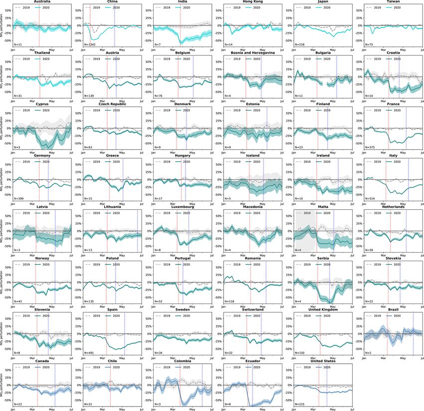
3556 C. A. Keller et al.: Global impact of COVID-19 restrictions
Petetin et al., 2020; Tobias et al., 2020; Le et al., 2020). NOx
has a short atmospheric lifetime and are predominantly emit-
ted during the combustion of fossil fuel for industry, trans-
port, and domestic activities (Streets et al., 2013; Duncan et
al., 2016). Atmospheric concentrations of nitrogen dioxide
(NO2 ) thus readily respond to local changes in NOx emis-
sions (Lamsal et al., 2011). While this may provide both
air quality and climate benefits, a quantitative assessment of
the magnitude of these impacts is complicated by the natural
variability of air pollution due to variations in synoptic con-
ditions (weather), seasonal effects, and long-term emission
trends, as well as the nonlinear responses between emissions
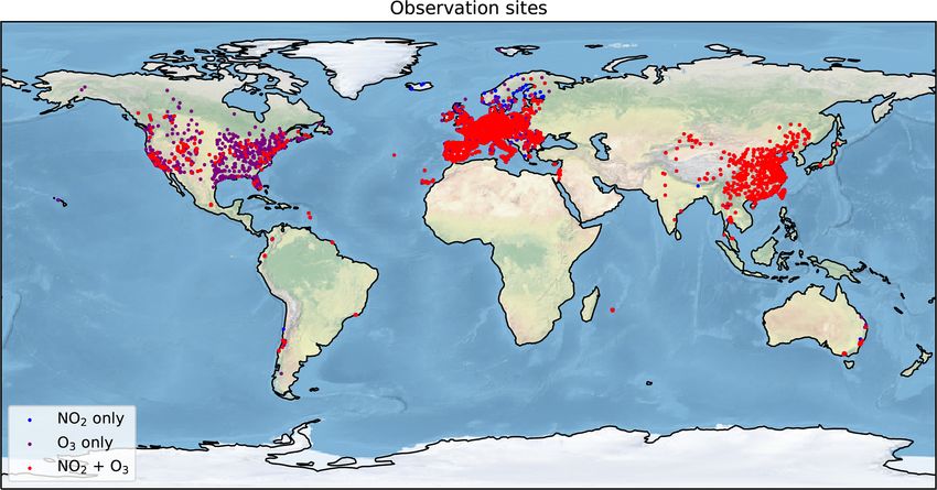
Figure 1. Location of the 5756 observation sites included in the
and concentrations. Thus, simply comparing the concentra-
analysis. Red points indicate sites with both NO2 and O3 observa-
tion of pollutants during the COVID-19 period to those im- tions (3485 in total), purple points show locations with O3 obser-
mediately beforehand or to the same period in previous years vations only (978 sites), and blue points show locations with NO2
is not sufficient to indicate causality. An emerging approach observations only (1293 sites). See the Appendix for detailed maps
to address this problem is to develop machine-learning-based for North America, Europe, and China.
“weather-normalization” algorithms to establish the relation-
ship between local meteorology and air pollutant surface
concentrations (Grange et al., 2018; Grange and Carslaw, 2 Methods
2019; Petetin et al., 2020). By removing the meteorological
influence, these studies have tried to better quantify emission 2.1 Observations
changes as a result of a perturbation.
Here, we adapt this weather-normalization approach to Our analysis builds on the recent development of unprece-
not only include meteorological information but also com- dented public access to air pollution model output and air
positional information in the form of the concentrations and quality observations in near-real time. We compile an air
emissions of chemical constituents. Using a collection of sur- quality dataset of hourly surface observations for a total of
face observations of NO2 and ozone (O3 ) from across the 5756 sites (4778 for NO2 and 4463 for O3 ) in 46 countries
world from 2018 to July 2020 (Sect. 2.1), we develop a for the time period 1 January 2018 to 1 July 2020, as sum-
“bias-correction” methodology for the NASA global atmo- marized in Fig. 1 and Table 1. More detailed maps of the
spheric composition model GEOS-CF (Sect. 2.2), which cor- spatial distribution of observation sites over China, Europe,
rects the model output at each observational site based on and North America are given in Figs. A1–A3. The vast ma-
the observations for 2018 and 2019 (Sect. 2.3). These biases jority of the observations were obtained from the OpenAQ
reflect errors in emission estimates, sub-grid-scale local in- platform and the air quality data portal of the European En-
fluences (representational error), or meteorology and chem- vironment Agency (EEA). Both platforms provide harmo-
istry. Since the GEOS-CF model makes no adjustments to the nized air quality observations in near-real time, greatly facil-
anthropogenic emissions in 2020, and no 2020 observations itating the analysis of otherwise disparate data sources. For
are included in the training of the bias corrector, the bias- the EEA observations, we use the validated data (E1a) for
corrected model (hereafter BCM) predictions for 2020 rep- the years 2018–2019 and revert to the real-time data (E2a)
resent a business-as-usual scenario at each observation site for 2020. For Japan, we obtained hourly surface observations
that can be compared against the actual observations. This al- for a total of 225 sites in Hokkaido, Osaka, and Tokyo from
lows the impact of COVID-19 containment measures on air the Atmospheric Environmental Regional Observation Sys-
quality to be explored, taking into account meteorology and tem (AEROS) (MOE, 2020). To improve data coverage in
the long-range transport of pollutants. We first apply this to under-sampled regions, we also included observations from
the concentration of NO2 (Sect. 3.1) and then O3 (Sect. 3.2) the cities of Rio de Janeiro (Brazil), Quito (Ecuador), and
and explore the differences between the counterfactual pre- Melbourne (Australia). All cities offer continuous, hourly
diction and the observed concentrations. In Sect. 3.3, we ex- observations of NO2 and O3 over the full analysis period,
plore how the observed changes in the NO2 concentrations thus offering an excellent snapshot of air quality at these lo-
relate to emission of NOx , and in Sect. 3.4 we speculate what cations. We include all sites with at least 365 d of observa-
the COVID-19 restrictions might mean for the second half of tions between 1 January 2018 and 31 December 2019 and
2020. an overall data coverage of 75 % or more since the first day
of availability. Only days with at least 12 h of valid data are
included in the analysis. The final NO2 and O3 dataset com-
prise 8.9 × 10⁷ and 8.2 × 10⁷ hourly observations, respec-
tively.
Atmos. Chem. Phys., 21, 3555–3592, 2021 https://doi.org/10.5194/acp-21-3555-2021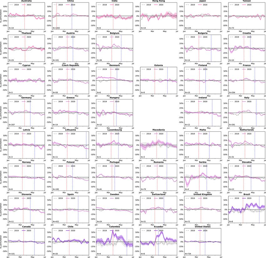
C. A. Keller et al.: Global impact of COVID-19 restrictions 3557
2.2 Model
Meteorological and atmospheric chemistry information at
each of the air quality observation sites is obtained from the
NASA Goddard Earth Observing System Composition Fore-
cast (GEOS-CF) model (Keller et al., 2020). GEOS-CF inte-
https://discomap.eea.europa.eu/map/fme/AirQualityExport.htm
grates the GEOS-Chem atmospheric chemistry model (v12-
01) into the GEOS Earth System Model (Long et al., 2015;
Hu et al., 2018) and provides global hourly analyses of atmo-
http://www.quitoambiente.gob.ec/ambiente/index.php
spheric composition at 25 × 25 km2 spatial resolution, avail-
able in near-real time at https://gmao.gsfc.nasa.gov/weather_
prediction/GEOS-CF/data_access/, last access: 5 July 2020
http://sciwebsvc.epa.vic.gov.au/aqapi/Help (Knowland et al., 2020). Anthropogenic emissions are pre-
http://www.data.rio/datasets/dados-hor
http://soramame.taiki.go.jp/Index.php
scribed using monthly Hemispheric Transport of Air Pol-
lution (HTAP) bottom-up emissions (Janssens-Maenhout et
al., 2015), with imposed weekly and diurnal scale factors as
described in Keller et al. (2020). The same anthropogenic
(last access: 3 July 2020)
(last access: 3 July 2020)
(last access: 4 July 2020)
(last access: 4 July 2020)
(last access: 4 July 2020)
(last access: 4 July 2020)
base emissions are used for the years 2018–2020. Therefore,
GEOS-CF does not account for any anthropogenic emission
https://openaq.org/
changes since 2018, notably any anthropogenic emission re-
ductions related to COVID-19 restrictions. However, it does
capture the variability in natural emissions such as wildfires
(based on the Quick Fire Emissions Dataset, QFED) (Dar-
Source
menov and Da Silva, 2015) or lightning and biogenic emis-
Table 1. Observational data sources used in the analysis. Time period covers 1 January 2018–1 July 2020.
sions (Keller et al., 2014). While the meteorology and strato-
spheric ozone in GEOS-CF are fully constrained by pre-
Sites
2410
3101
225
4
8
8
computed analysis fields produced by other GEOS systems
(Lucchesi, 2015; Wargan et al., 2015), no trace gas obser-
Australia, China, India, Hong Kong, Taiwan, Thailand, Canada,
Austria, Belgium, Bosnia and Herzegovina, Bulgaria, Croatia,
Cyprus, Czech Republic, Denmark, Estonia, Finland, France,
Germany, Greece, Hungary, Iceland, Ireland, Italy, Latvia,
Lithuania, Luxembourg, North Macedonia, Malta, Netherlands,
Norway, Poland, Portugal, Romania, Serbia, Slovakia, Slove-
vations are directly assimilated into the current version of
GEOS-CF. It thus provides a “business-as-usual” estimate of
NO2 and O3 that can be used as a baseline for input into the
meteorological normalization process.
nia, Spain, Sweden, Switzerland, United Kingdom
2.3 Machine learning bias correction
2.3.1 Overall strategy
We use the XGBoost machine learning algorithm
Chile, Colombia, United States
(https://xgboost.readthedocs.io/en/latest/#, last access:
15 March 2020) (Chen and Guestrin, 2016; Frery et al.,
2017) to develop a machine learning model to predict the
Brazil (Rio de Janeiro)
Australia (Melbourne)
time-varying bias at each observation site at an hourly
scale. XGBoost uses the Gradient Boosting framework to
Ecuador (Quito)
build an ensemble of decision trees, trained iteratively on
the residual errors to improve the model predictions in a
Countries
stagewise manner (Friedman, 2001). Based on the 2018–
Japan
2019 observation–model differences, the machine learning
model is trained to predict the systematic (recurring) model
bias between hourly observations and the co-located model
Municipal Government
predictions. These biases can be due to errors in the model,
such as emission estimates, sub-grid-scale local influences
of Rio de Janeiro
Ambiente, Quito
(representational error), or meteorology and chemistry.
EPA Victoria
Secretaria de
Since model biases are often site-specific, we train a separate
OpenAQ
AEROS
machine learning model for each site.
Name
EEA
https://doi.org/10.5194/acp-21-3555-2021 Atmos. Chem. Phys., 21, 3555–3592, 2021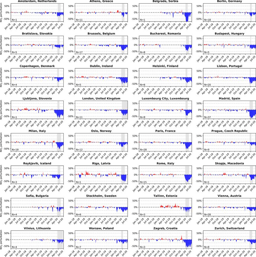
3558                                                               C. A. Keller et al.: Global impact of COVID-19 restrictions

   The design of the XGBoost framework is determined by              lutants. In addition, for sites with observations available for
a set of hyperparameters, such as the learning rate, maxi-           the full two years, we provide the calendar days since 1 Jan-
mum tree depth, or minimum loss reduction. While a full              uary 2018 as an additional input feature to also correct for
hyperparameter optimization across all sites – e.g., by us-          inter-annual trends in air pollution, e.g., due to a steady de-
ing a grid search approach – would be computationally pro-           crease in emissions not captured by the model. This follows
hibitive, we conducted hyperparameter sensitivity tests at           a similar technique to Ivatt and Evans (2020) and Petetin et
few selected sites and found that the XGBoost performance            al. (2020).
only improved marginally at these sites when using hyper-               Gradient-boosted tree models consist of a tree-like deci-
parameters other than the model defaults (less than 5 % im-          sion structure, which can be analyzed to understand how the
provement). In addition, we found that the sites respond dif-        model uses the input features to make a prediction. Partic-
ferently to the same change in hyperparameter setup, sug-            ularly useful in this context is the SHapely Additive exPla-
gesting that there is no uniform hyperparameter design that          nations (SHAP) approach, which is based on game-theoretic
is optimal across all sites. Based on this, we chose to use the      Shapely values and represents a measure of each feature’s re-
default XGBoost model parameters at all locations, with a            sponsibility for a change in the model prediction (Lundberg
learning rate of 0.3, minimum loss reduction of 0, maximum           et al., 2017). SHAP values are computed separately for each
tree depth of 6, and L1 and L2 regularization terms of 0 and         individual model prediction, offering detailed insight into the
1, respectively.                                                     importance of each input feature to this prediction while also
   For each location, we split the 2-year training dataset into      considering the role of feature interactions (Lundberg et al.,
eight quarterly segments (January–March, April–June, etc.)           2020). In addition, combining the local SHAP values offers a
and train the model eight times, each time omitting one of           representation of the global structure of the machine learning
the segments (8-fold cross validation). The omitted segment          model.
is used as test data to validate the general performance of the         Figure A4 shows the distribution of the SHAP values for
machine learning model and to provide an uncertainty esti-           all NO2 predictors separated by polluted sites (left panel)
mate, as is further discussed below. This approach aims to           and non-polluted sites (right panel), with polluted sites de-
reduce the auto-correlation signal that can lead to overly op-       fined as locations with an annual average NO2 concentration
timistic machine learning results (Kleinert et al., 2021), while     of more than 15 ppbv. Generally, the model-predicted (un-
still including data from all four seasons in the testing. Once      biased) NO2 concentration is the most important predictor
trained, the final model prediction at each location consists        for the model bias, followed by the hour of the day, the day
of the average prediction of the eight models.                       since 1 January 2018 (“trendday”), and a suite of meteorolog-
   The observations used in this analysis are not always             ical variables including wind speed (u10m, v10m), planetary
quality-controlled, which can cause issues if erroneous ob-          boundary hight (zpbl), and specific humidity (q10m). All of
servations are included in the training, such as unrealistically     these factors are expected to highly impact NO2 concentra-
high O3 concentrations of several thousand parts per billion         tions and it is thus not surprising that the model biases are
by volume. As an ad hoc solution to this problem, we re-             most sensitive to them. While there is considerable spread in
move all observations below or above 2 standard deviations           the feature importance across the individual sites, there is lit-
from the annual mean from the analysis. Sensitivity tests us-        tle overall difference in the feature ranking between polluted
ing more stringent thresholds of 3 or even 4 standard devia-         vs. non-polluted sites.
tions resulted in no significant change in our results.                 Figure A5 shows the SHAP value distribution for all O3
                                                                     predictors, again separated into polluted and non-polluted
2.3.2   Evaluation of model predictors                               sites (using the same definition as for the NO2 sites). Unlike
                                                                     for NO2 , the bias-correction models for polluted sites exhibit
The input variables fed into the XGBoost algorithm are pro-          different feature sensitivities than the non-polluted sites. At
vided in Table A1. The input features encompass 9 meteo-             polluted locations, the availability of reactive nitrogen (NO2 ,
rological parameters (as simulated by the GEOS-CF model:             NOy , PAN) is the dominant factor for explaining the model
surface northward and eastward wind components, surface              O3 bias, reflecting the tight chemical coupling between NOx
temperature and skin temperature, surface relative humidity,         and O3 (Seinfeld and Pandis, 2016). This is followed by the
total cloud coverage, total precipitation, surface pressure, and     month of the year, total precipitation (tprec), and O3 concen-
planetary boundary layer height), modeled surface concen-            tration, again variables that are expected to be correlated to
trations of 51 chemical species (O3 , NOx , carbon monoxide,         O3 . At non-polluted sites, the uncorrected O3 concentration
volatile organic compounds (VOCs), and aerosols), and 21             is on average the most relevant input feature for the bias cor-
modeled emissions at the given location. In addition, we pro-        rectors, followed by the month of the year and the odd oxy-
vide as input features the hour of the day, day of the week,         gen concentration (Ox =NO2 +O3 ). The non-polluted sites are
and month of the year; these allow the machine learning              generally more sensitive to wind speed, reflecting the fact
model to identify systematic observation–model mismatches            that O3 production and loss at these locations is less domi-
related to the diurnal, weekly, and seasonal cycle of the pol-       nated by local processes compared to the polluted sites.

Atmos. Chem. Phys., 21, 3555–3592, 2021                                                https://doi.org/10.5194/acp-21-3555-2021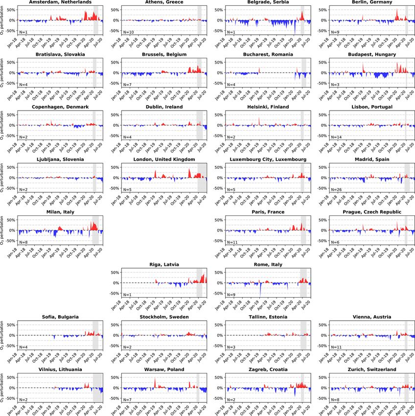
C. A. Keller et al.: Global impact of COVID-19 restrictions                                                                  3559

2.3.3   Machine learning model skill scores                        ties are adjusted accordingly by calculating the mean uncer-
                                                                   tainty σ from the above-described hourly uncertainties σi :
Figures 2 and 3 summarize the machine learning model                      XN  σi 2
statistics for NO2 and O3 , respectively. The normalized mean      σ2 =      i=1 N
                                                                                       .                                     (1)
bias (NMB), normalized root-mean-square error (NRMSE),
and Pearson correlation coefficient (R) at each site are shown     This assumes that the errors across individual sites are un-
for both the training (blue) and the test (red) dataset. We de-    correlated. The error covariance across sites is complex: two
fine NMB as mean bias normalized by average concentration          urban sites close to each other might show a low degree of
at the given site, and the NRMSE as the root-mean-square           error correlation due to local-scale (street, canyon, etc.) dif-
error normalized by the range of the 95th percentile concen-       ferences, whereas two background sites further apart might
tration and 5th percentile concentration. Rather than using        show significantly more correlation due to regional-scale
the mean as the denominator for the NRMSE, we choose the           (synoptic) processes. In addition, our uncertainty calculation
percentile window as a better reference point for the concen-      also implies that the aggregated mean error approaches zero.
tration variability at a given site. Using the mean as the de-     Given that the average mean biases of the machine learn-
nominator for the NRMSE would lead to very similar quali-          ing models are clustered around zero (Figs. 2 and 3), this
tative results.                                                    is a valid general assumption – especially when aggregating
   For both NO2 and O3 , the bias-corrected model predic-          across multiple sites. For simplicity we keep the current anal-
tions show no bias when evaluated against the training data,       ysis but acknowledge that it might lead to overly optimistic
NRMSEs of less than 0.3, and correlation coefficients be-          uncertainty estimates for sites with a relatively large mean
tween 0.6–1.0 (NO2 ) and 0.75–1.0 (O3 ). Compared to the           bias.
training data, the skill scores on the test data show a higher
variability, with an average NMB of −0.047 for NO2 and             2.4    Lockdown dates
−0.034 for O3 , a NRMSE of 0.25 (NO2 ) and 0.18 (O3 ), and
a correlation of 0.64 (NO2 ) and 0.84 (O3 ). We find no signif-    To support interpretation and guide visualizations, we
icant difference in skill scores between background vs. pol-       include approximate national lockdown dates in all fig-
luted sites or different countries.                                ures. The start and end dates for these are from https:
   A number of factors likely contribute to the poorer statisti-   //en.wikipedia.org/wiki/COVID-19_pandemic_lockdowns,
cal results at some of the sites. Importantly, some sites might    last access: 1 July 2020 (as of 1 July 2020) or based on
be prone to overfitting if the training data include events that   local knowledge, with the full list of start and end dates
are not easily generalizable, such as unusual emission activ-      given in Table A2. It should be noted that in many countries
ity (e.g., biomass burning, fireworks, closure of nearby point     lockdown policy varied regionally and that many locations
source) or weather patterns that are not frequently observed.      enacted “soft” stay-at-home orders before the official
In addition, the availability of test data at some locations is    lockdowns. Human behavior is therefore expected to have
weak (less than 50 %), which can contribute to a poorer skill      changed considerably in many locations before the official
score.                                                             lockdowns went into force.

2.3.4   Uncertainty estimation                                     3     Results
To quantify the uncertainty of an individual model predic-         3.1    Nitrogen dioxide
tions at any given site, we use the standard deviation of the
model-observation differences on the test data. For sites with     Figure 4 shows the weekly mean observations of NO2 con-
100 % test data coverage, this represents the standard devia-      centration, the GEOS-CF estimate, and the BCM prediction
tion from a sample of 17 520 hourly model-observation pairs.       based on the machine learning predictor trained on 2018–
The thus obtained individual NO2 prediction uncertainties          2019 for the five cities of Wuhan (China), Taipei (Taiwan),
range between 3.9–28 ppbv (mean = 8.5 ppbv) at polluted            Milan (Italy), New York (USA), and Rio de Janeiro (Brazil)
sites and 0.1–18 ppbv at clean sites (average of 4.9 ppbv). On     from January 2018 through June 2020. We choose these
a relative basis, this corresponds to an average uncertainty of    five cities for illustration as they represent a diverse level
45 % at polluted sites and 65 % at clean sites. For O3 , we ob-    of socio-economic development and due to the cities’ vari-
tain an average individual prediction uncertainty of 14 ppbv       able responses to the COVID-19 pandemic. These five cities
(4.6–33 ppbv) at polluted sites and 9.0 ppbv (2.8–45 ppbv) at      are also illustrative of the varying quality of the uncorrected
clean sites, corresponding to an average relative uncertainty      GEOS-CF predictions compared to the observations. For ex-
of an individual prediction of 29 % and 33 % at polluted and       ample, as shown by the dashed grey lines vs. the solid black
clean sites, respectively.                                         lines in Fig. 4, the uncorrected model predictions are in good
   The results presented in this paper are averages aggregated     agreement with observations in Rio de Janeiro but underes-
over multiple hours and locations, and the reported uncertain-     timate the observed NO2 concentrations in Taipei and Milan

https://doi.org/10.5194/acp-21-3555-2021                                            Atmos. Chem. Phys., 21, 3555–3592, 2021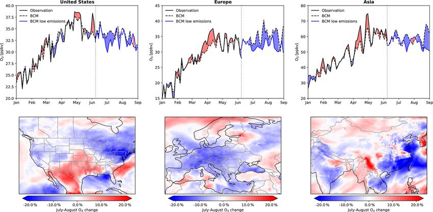
3560                                                                   C. A. Keller et al.: Global impact of COVID-19 restrictions

Figure 2. Machine learning statistics between hourly observations and the corresponding bias-corrected model predictions for each observa-
tion location. Shown are the normalized mean bias (NMB), normalized root-mean-square error (NRMSE), and Pearson correlation coefficient
(R) for the training data (blue) and the test data (red). Data are sorted by region: China, Europe, United States (USA), and rest of the world
(ROW). The mean values across all locations are shown in the figure inset.

Figure 3. The same as Fig. 2 but for O3 .

while overestimating concentrations over New York. These                 the start and end of the implementation of COVID-19 con-
differences are a combination of the observation–model scale             tainment measures. Once containment is implemented, ob-
mismatch (25 × 25 km2 vs. point observation) and model er-               served concentrations start to diverge from the BCM predic-
rors, such as the simulated spatiotemporal distribution of               tion for Wuhan, Milan, and New York (Fig. 4). For Wuhan,
NOx emissions or the modeling of the local boundary layer.               we find a reduction in NO2 of 54 (48–59) % relative to the
The model–observation mismatch is particularly pronounced                expected BCM value for February and March 2020, and av-
for Wuhan, where the model does not capture the observed                 erage decreases of 30 %–40 % are found over Milan (24 %–
seasonal cycle, pointing to errors in the imposed seasonal cy-           43 %) and New York (20 %–34 %) starting in mid-March
cle of NOx emissions in the model.                                       and lasting through April (Fig. 4; Tables A3–A5). For cities
   In contrast to the uncorrected model predictions, the BCM             where restrictions have been mainly removed (Wuhan, Mi-
closely follows the observations for years 2018 and 2019                 lan) concentrations rise back towards the BCM value, al-
(dashed black lines in Fig. 4). The grey region in Fig. 4 shows          though the concentrations in neither city have been fully re-

Atmos. Chem. Phys., 21, 3555–3592, 2021                                                     https://doi.org/10.5194/acp-21-3555-2021
C. A. Keller et al.: Global impact of COVID-19 restrictions                                                                         3561

Figure 4. Comparison of NO2 surface concentrations (ppbv = nmol mol−1 ) for Wuhan, Taipei, Milan, New York, and Rio de Janeiro for
January 2018 through June 2020. Observed values are shown in solid black, the original GEOS-CF model simulation is shown in dashed
grey, and the BCM predictions are in dashed black. The area between observations and BCM predictions is shaded blue (red) if observations
are lower (higher) than BCM predictions. Grey areas represent the period of lockdown. Shown are the 7 d average mean values for the 9,
18, 19, 14, and 2 observational sites in Wuhan, Taipei, Milan, New York, and Rio de Janeiro, respectively. Observations for China are only
available starting in mid-September 2018.

stored to what might be expected based on the business-as-             laxed containment measures in these places (Figs. A6–A8).
usual GEOS-CF simulation.                                              In contrast, Tokyo (Japan) and Stockholm (Sweden), which
   Looking more broadly at cities around the globe, 53 of the          also implemented a less aggressive COVID-19 response, ex-
64 specifically analyzed cities feature NO2 reductions of be-          hibit NO2 reductions comparable to those of cities with of-
tween 20 %–50 % (Figs. A6–A8 and Tables A3–A5). Most                   ficial lockdowns (>20 %), suggesting that economic and hu-
locations issued social distancing recommendations prior to            man activities were similarly subdued in those cities.
the legal lockdowns and observed NO2 declines often pre-                  Substantial differences exist between cities in South
cede the official lockdown date by 7–14 d (e.g., Brussels,             America, with Rio de Janeiro and Santiago de Chile show-
London, Boston, Phoenix, and Washington, D.C.).                        ing little change over the analyzed period, whereas Quito
   For Taipei and Rio de Janeiro, the observations and the             (Ecuador) and Medellín (Colombia) experienced a greater
BCM show little difference (Fig. 4), consistent with the less          than 50 % reduction in NO2 after the initiation of strict re-
stringent quarantine measures in these places. Other cities            strictions measures in mid-March (Fig. A8 and Table A5).
with only short-term NO2 reductions of less than 25 % in-              Concentrations in Medellín rebounded sharply in April and
clude Atlanta (USA), Prague (Czech Republic), and Mel-                 May, while concentrations in Quito remained 55 (52–58) %
bourne (Australia), again fitting with the comparatively re-

https://doi.org/10.5194/acp-21-3555-2021                                                 Atmos. Chem. Phys., 21, 3555–3592, 2021
3562                                                               C. A. Keller et al.: Global impact of COVID-19 restrictions

below business as usual throughout May and only started to           NO2 declines comparable to Wuhan or Milan (Figs. A9–
return back to normal in June.                                       A11). O3 enhancements of up to 20 % are found over Europe
   To evaluate the large-scale impact of COVID-19 restric-           (e.g., Belgium, Luxembourg, Serbia), with a peak in early
tions on air quality, we aggregate the individual observation–       April, approximately 2 weeks after lockdown started (Fig. 7).
model comparisons by country. We note that our estimates                The analysis of O3 is complicated by its nonlinear chem-
for some countries (e.g., Brazil, Colombia) are based on a           ical response to NOx emissions. In the presence of sunlight,
single city and likely not representative of the whole coun-         O3 is produced chemically from the oxidation of volatile or-
try. On a country level, we find the sharpest and earliest drop      ganic compounds in the presence of NOx (Seinfeld and Pan-
in NO2 over China, where observed concentrations fell, on            dis, 2016). Therefore, a decline in NOx emissions could de-
average, 55 (51–59) % below their expected value in early            crease O3 production and thus suppress O3 concentrations.
February when restrictions were implemented (Fig. 5). Con-           On the other hand, the process of NOx titration, in which
centrations remained at this level until late February, at which     freshly emitted NO rapidly reacts with O3 to form NO2 , acts
point they started to increase until restrictions were signifi-      as a sink for O3 (Seinfeld and Pandis, 2016). Odd oxygen
cantly relaxed in early April. Our analysis suggests that Chi-       (Ox ) is conserved when O3 reacts with NO and thus of-
nese NO2 concentrations have recovered to within 5 (1–9) %           fers a tool for separating these competing processes. Fig-
of the business-as-usual values since then. For 2019 (dashed         ure 8 presents the global mean diurnal cycle for O3 and
line in Fig. 5) the BCM shows a reduction in NO2 con-                Ox for the 5-month period since 1 February 2020 for both
centrations around Chinese New Year (5 February 2019),               the observations and the BCM model, based on the individ-
and it is likely that some reduction around the equivalent           ual hourly predictions at each observation site aggregated
2020 period (25 January 2020) would have occurred anyway.            by local hour. The analysis of O3 and Ox is based on the
However, the 2020 reductions are significantly larger and            same set of observation sites where both NO2 and O3 ob-
more prolonged than in 2019. Similar to China, India shows           servations are available (see Fig. 1). Compared to the BCM
large reductions in NO2 concentration (58 (49–67) %) coin-           model, there has been an increase in the concentration of
ciding with the implementation of restrictions in mid-March          nighttime O3 (00:00–05:00 LT, local time, Fig. 8a) by 1 ppbv
(Fig. 5); however, NO2 concentrations have not yet recovered         (ppbv = nmol mol−1 ) compared to the BCM, whereas Ox
by the end of June, reflecting the prolonged duration of lock-       shows a decrease of 1 ppbv (Fig. 8b). While these changes
down measures. Other areas of Asia, such as Hong Kong and            are small in magnitude, they represent a multi-month aggre-
Taipei, implemented smaller restrictions than China or In-           gate over 3485 observation sites that are statistically signif-
dia and they show significantly smaller decreases (less than         icant at the 1 % confidence interval. It should be noted that
20 %).                                                               the biases of the machine learning models show little diurnal
   For Europe and the United States, we find widespread NO2          variability (Figs. A12–13), suggesting that this result is not
reductions averaging 22 (19–25) % in March and 33 (30–               caused by poor model performance during specific times of
36) % in April (Fig. 5). In some countries, recovery is evi-         the day.
dent as lockdown restrictions are removed or lessened (e.g.,            Our results indicate that during the night reduced NO
Greece, Romania), but in 29 out of 36 countries concentra-           emissions led to a reduction in O3 titration, allowing O3 con-
tions remain 20 % or more below the business-as-usual sce-           centrations to increase. During the afternoon, we find that O3
nario throughout May and June.                                       concentrations are lower by 1 ppbv (Fig. 8a), while observed
                                                                     Ox concentrations are lower than the baseline model by al-
3.2    Ozone                                                         most 2 ppbv at 14:00 LT (Fig. 8b). We attribute the lower Ox
                                                                     to reduced net Ox production due to the lower NOx concen-
We follow the same methods for developing a business-as-             tration, but as titration is also reduced, daytime O3 concen-
usual counterfactual for O3 as we did for NO2 in Sect. 3.1.          trations change little. Overall changes to mean O3 concentra-
Any change in local O3 concentration arising from COVID-             tions are small, but there is a flattening of the diurnal cycle.
19 restrictions is set against a large seasonal increase in             As shown in the lower panels in Fig. 8, both factors – en-
(background) concentrations in the Northern Hemisphere               hanced nighttime O3 and reduced daytime Ox – are more
springtime (Fig. 6). Due to the longer atmospheric lifetime          pronounced at locations where preexisting NO2 concentra-
of O3 compared to NO2 , the local O3 signal is expected to           tions are high (>15 ppbv). This suggests that the observed
be comparatively small. This makes attributing changes in            O3 deviations from the BCM are indeed coupled to NOx re-
O3 concentration more challenging than for NO2 . Our anal-           ductions due to COVID-19 restrictions, given that those are
ysis shows an O3 increase of up to 50 % for some periods in          most pronounced at polluted sites.
cities with large NO2 reductions (e.g., Wuhan, Milan, Quito;
Figs. 3 and A9–A11), but there is much less convincing ev-           3.3   NOx emission reductions
idence for a systematic O3 response across cities or on a re-
gional level (Fig. 7). For example, our analysis shows little        The NO2 analysis presented in Sect. 3.1 implies a stark re-
O3 difference in Beijing and Madrid during lockdown despite          duction in NOx emissions. However, due to the impact of

Atmos. Chem. Phys., 21, 3555–3592, 2021                                                https://doi.org/10.5194/acp-21-3555-2021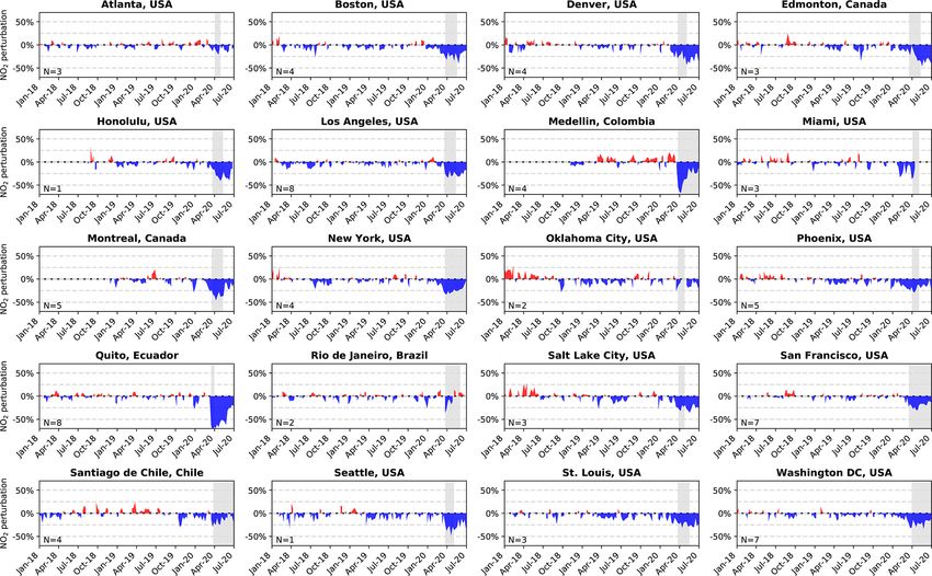
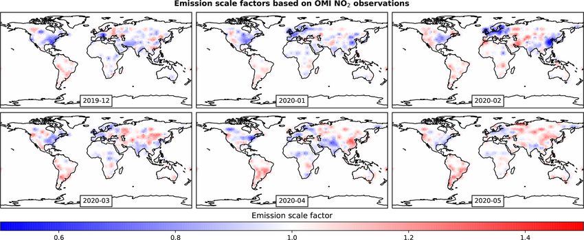
C. A. Keller et al.: Global impact of COVID-19 restrictions                                                                                3563

Figure 5. The 7 d average fractional difference between observed NO2 and the BCM predictions for 46 countries between 1 January through
30 June, aggregated from all sites across each country (number of sites given at the bottom left of each panel). The thick line indicates the
mean across all sites for the first half of 2020, with the shaded area representing the uncertainty estimate. Differing colors indicate differing
regions (cyan: Asia and Australia; green: Europe; blue: Americas). The dashed grey line indicates the equivalent average for the same 6 month
period in 2019 (note that 2019 data was included in the training). The dashed vertical red line indicates COVID-19 restriction dates, and the
blue line indicates the beginning of easing measures.

atmospheric chemistry, changes in NO2 concentrations do                    ring NOx emissions from NO2 concentrations (Lamsal et al.,
not reflect the same relative change in NOx emissions. Be-                 2011; Shah et al., 2020). To estimate the relationship be-
cause of this, the NO2 / NOx ratio and the NOx lifetime,                   tween changes in NOx emission and changes in NO2 con-
both of which depend on seasonality and the local chemi-                   centrations, we conducted a sensitivity simulation for the
cal environment, need to be taken into account when infer-                 time period 1 December 2019 to 8 June 2020 using the

https://doi.org/10.5194/acp-21-3555-2021                                                      Atmos. Chem. Phys., 21, 3555–3592, 2021
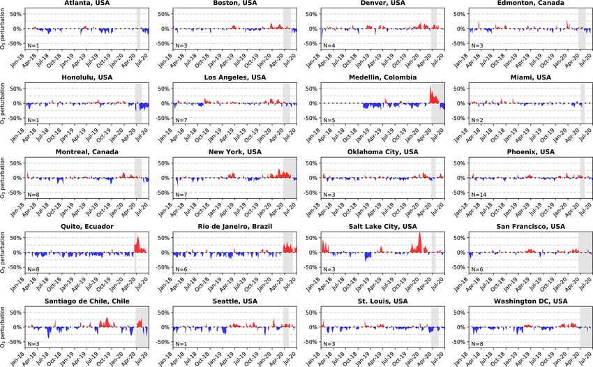
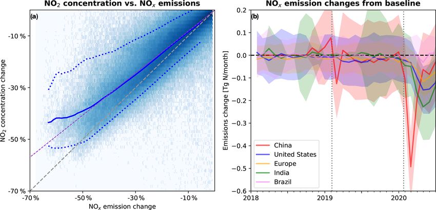
3564                                                                 C. A. Keller et al.: Global impact of COVID-19 restrictions

Figure 6. Comparison of O3 surface concentrations for Wuhan, Taipei, Milan, New York, and Rio de Janeiro for January 2018 through
June 2020. Observed values are shown in solid black, the original GEOS-CF model simulation is shown in dashed grey, and the BCM
predictions are in dashed black. The area between observations and BCM predictions is shaded blue (red) if observations are lower (higher)
than BCM predictions. The grey areas represent the period of lockdown. Shown are the 7 d average mean values for the 9, 18, 19, 14, and 4
observational sites in Wuhan, Taipei, Milan, New York, and Rio de Janeiro, respectively. Observations for China are only available starting
in mid-September 2018.

GEOS-CF model with perturbed anthropogenic emissions.                   factors do not necessarily coincide in space and time with
The perturbation simulation uses anthropogenic NOx emis-                the ones derived from observations and the BCM, and they
sions scaled based on adjustment factors derived from NO2               do not include any adjustment for the NO2 / NOx ratio.
tropospheric columns observed by the NASA OMI instru-                      Figure 9a shows the response of NO2 surface concentra-
ment (Boersma et al., 2011). Daily scale factors were com-              tion to a change in NOx emissions derived from the com-
puted by normalizing coarse-resolution (2 × 2.5◦ ) 14 d NO2             parison of the sensitivity experiment against the GEOS-CF
tropospheric column moving averages by the corresponding                reference simulation. Our results indicate that NO2 concen-
moving average for year 2018 (the emissions base year in                trations drop, on average, by 80 % of the fractional decrease
GEOS-CF; Sect. 2.2). Forest fire signals were filtered out              in anthropogenic NOx emission, with a further diminishing
based on QFED emissions and no scaling was applied over                 effect for emission reductions greater than 50 %. This reflects
water. This results in anthropogenic emission adjustment fac-           both the buffering effect of atmospheric chemistry and the
tors of 0.3 to 1.4 (Fig. A14), comparable to the magnitude              presence of natural background NO2 . The here-derived aver-
obtained from the observation–BCM comparisons at cities                 age sensitivity of 0.8 between a change in surface NO2 to a
globally (Fig. 5) and capturing the range of expected NOx               change in NOx emissions is comparable to the value of 0.86
emission changes. However, it should be noted that the scale            (1/1.16) obtained by Lamsal et al. (2011) for the relation-

Atmos. Chem. Phys., 21, 3555–3592, 2021                                                    https://doi.org/10.5194/acp-21-3555-2021
C. A. Keller et al.: Global impact of COVID-19 restrictions                                                                        3565

Figure 7. Similar to Fig. 5 but for O3 and without Bosnia and Herzegovina and Iceland. Differing colors indicate differing regions (pink:
Asia and Australia; light purple: Europe; dark purple: Americas).

ship between NOx emissions and tropospheric column NO2                 sensitivity (Fig. 9a). This is a simplification, as the local
observations.                                                          NOx / NO2 sensitivity ratio is highly dependent on the lo-
   To infer the reduction in anthropogenic NOx emissions               cal environment. To account for this uncertainty, we assign
due to COVID-19 containment measures during the first 6                an absolute error of 15 % to our NOx / NO2 sensitivity, as
months of 2020, we use the best linear fit between the sim-            derived from the spread in the NOx / NO2 ratio in the sensi-
ulated NOx / NO2 sensitivity (dashed purple line in Fig. 9a).          tivity simulation (Fig. 9a). We then aggregate these estimates
To do so, we calculate the monthly percentage emission                 to a country level by weighting them based on average NO2
change at each observation site based on the NO2 anomalies             concentrations per location, thus giving higher weight to lo-
derived in Sect. 3.1 and the corresponding best fit NOx / NO2          cations with more nearby NOx emission sources. It should be

https://doi.org/10.5194/acp-21-3555-2021                                                 Atmos. Chem. Phys., 21, 3555–3592, 2021
3566                                                               C. A. Keller et al.: Global impact of COVID-19 restrictions

Figure 8. Observed and BCM-modeled diurnal cycle of O3 (a) and Ox (b) averaged across all surface observation sites between 1 Febru-
ary 2020 through 30 June 2020 with estimated corresponding changes in surface O3 (c) and Ox (d) relative to the BCM. Bar plots (c and
d) show observed changes during nighttime (0:00–05:00 LT) and the afternoon (12:00–17:00 LT) for locations with low (15 ppbv) NO2 concentrations (based on the 2019 average).

noted that for some countries our estimates are based upon a          sions (excluding international shipping and aviation). We
small number of observation sites that might not be repre-            have no information for significant countries such as Rus-
sentative for the country as a whole. This is particularly true       sia, Indonesia, or anywhere in Africa due to the lack of pub-
for India and Brazil, where less than 10 observation sites are        licly available near-real-time air quality information. China
available. While the smaller observation sample size is re-           accounts for the largest fraction of the total deduced emis-
flected in the wider uncertainty associated with these emis-          sion reductions (28 %), followed by India (25 %), the United
sion estimates compared to countries with a much denser               States (18 %), and Europe (12 %).
monitoring network (e.g., China or Europe), the applied ex-              While our method does not allow for sector-specific emis-
trapolation method might incur errors that are not reflected          sion attribution, we assume our results to be most represen-
in the stated uncertainty ranges.                                     tative for changes in traffic emissions (rather than say air-
   To obtain absolute estimates in emission changes, the              craft emissions) given the location of the observation sites.
monthly country-level percentage emission changes are con-            On average, traffic emissions represent 27 % of total anthro-
voluted with bottom-up emissions estimates for 2015 from              pogenic NOx emissions (Crippa et al., 2018), and our derived
the Emission Database for Global Atmospheric Research                 total NOx emission reduction from January–June 2020 cor-
(EDGAR v5.0_AP; Crippa et al., 2018, 2020). The choice                responds to 21 (17–24) % of global annual traffic emissions.
of EDGAR v5.0 as the bottom-up reference inventory (over,             The share of transportation on total NOx emissions is higher
e.g., the HTAP emissions inventory used in GEOS-CF) was               in the US and Europe (approx. 40 %) compared to India and
motivated by the fact that its baseline has been updated more         China (20 %–25 %). Taking this into account, the derived ra-
recently and the country emission totals – which our analysis         tio of NOx emission reductions to annual traffic emissions
is based on – are readily available.                                  is 21 (16–26) % in the US, 25 (20–30) % in Europe, 39 (34–
   As summarized in Table 2, we calculate that the total re-          44) % in China, and 62 (55–69) % in India.
duction in anthropogenic NOx emissions due to COVID-
19 containment measures during the first 6 months of 2020             3.4   Long-term impact of reduced NOx emissions on
amounted to 3.1 (2.6–3.6) TgN (Fig. 9b and Table 2). This is                surface O3
equivalent to 5.5 (4.7–6.4) % of global annual anthropogenic
NOx emissions (Table 2). Our estimate encompasses 46                  The response of O3 to NO2 declines in the wake of the
countries that together account for 67 % of the total emis-           COVID-19 outbreak is complicated by the competing in-

Atmos. Chem. Phys., 21, 3555–3592, 2021                                                 https://doi.org/10.5194/acp-21-3555-2021
C. A. Keller et al.: Global impact of COVID-19 restrictions                                                                             3567

Figure 9. (a) Response of NO2 surface concentration (y axis) to a change in NOx emissions (x axis), as deduced from a model sensitivity
simulation (see methods). The solid blue line shows the mean value across all individual grid cells (blue squares) and the dotted blue lines
show the 5 % and 95 % quantiles. The dashed purple line shows the best linear fit. (b) Estimated monthly change in NOx emissions from the
baseline since 2018 for China (red), the United States (blue), Europe (yellow), India (green), and Brazil (purple), as estimated from observed
NO2 concentration anomalies. Shaded areas indicate estimated emission uncertainties. Dotted grey lines indicate Chinese New Year 2019
and 2020.

fluences of atmospheric chemistry. From February through                    Figure 10 shows the differences between the reference
June 2020, the diurnal observation-BCM comparisons sug-                  forecast and the sensitivity simulation over the United States,
gest that the reduction in photochemical production was off-             Europe, and China. Our results indicate that sustained lower
set by a smaller loss from titration, as described in Sect. 3.2.         anthropogenic emissions lead to a general decrease in surface
This resulted in a flattening of the diurnal cycle and an in-            O3 concentrations of 10 %–20 % over eastern China, Europe,
significant net change in surface O3 over a diurnal cycle. The           and the western and northeastern US during July and August
competing impacts of reduced NOx emissions on O3 produc-                 relative to the business-as-usual reference forecast simula-
tion and loss are dependent on the local chemical and mete-              tion. However, it is also notable that in some locations the
orological environment. This is reflected in the variable ge-            model forecast O3 concentrations increase by an equivalent
ographical response of O3 following the implementation of                amount (e.g., Scandinavia, southern central US and Mex-
COVID-19 restrictions (Le et al., 2020; Dantas et al., 2020).            ico, northern India), reflecting the high nonlinearity of atmo-
Moreover, as atmospheric reactivity increases through the                spheric chemistry. This highlights the complex interactions
Northern Hemisphere spring and summer, the relative impor-               between emissions, chemistry, and meteorology and their im-
tance of photochemical production is expected to increase in             pact on air pollution on different time scales.
the Northern Hemisphere.
   To assess the potential seasonal-scale impact of reduced
anthropogenic emissions on O3 , we conducted two free-                   4    Conclusions
running forecast simulations between 8 June and 31 Au-
gust 2020, initialized from the GEOS-CF simulation and                   The combined interpretation of observations and model sim-
the sensitivity simulation described in Sect. 3.3, respectively.         ulations using machine learning can be used to remove the
Both simulations use the same biomass burning emissions                  confounding effect of meteorology and atmospheric chem-
based on a historical QFED climatology. For the forecast                 istry, offering an effective tool to monitor and quantify
sensitivity experiment, we assume a sustained, time-invariant            changes in air pollution in near-real time. The global re-
20 % reduction in global anthropogenic emissions of NOx ,                sponse to the COVID-19 pandemic presents a perfect test
carbon monoxide (CO), and VOCs. We chose to alter not                    bed for this type of analysis, offering insights into the in-
only the anthropogenic emissions of NOx but also other pol-              terconnectedness of human activity and air pollution. While
lutants whose anthropogenic emissions are highly correlated              national mitigation strategies have led to substantial re-
to NOx , as a reduction in NOx emissions without corre-                  gional NO2 concentration decreases over the past decades
sponding declines in CO and VOC emissions seems unre-                    in many places (e.g., Hilboll et al., 2013; Russell et al.,
alistic.                                                                 2012; Castellanos and Boersma, 2012), the widespread and
                                                                         near-instantaneous reduction in NO2 following the imple-

https://doi.org/10.5194/acp-21-3555-2021                                                    Atmos. Chem. Phys., 21, 3555–3592, 2021
3568 C. A. Keller et al.: Global impact of COVID-19 restrictions
Table 2. Anthropogenic NOx emission reductions in GgN month−1 as derived from NO2 concentration changes.
Baselinea Feb 2020 Mar 2020 Apr 2020 May 2020 Jun 2020
Australia 621 −2.9 (−13.8–8.0) −3.7 (−14.4–6.9) −8.5 (−18.5–1.6) −6.1 (−16.1–3.8) −7.9 (−17.6–1.8)
Austria 73 −0.5 (−1.4–0.5) −1.7 (−2.7– −0.7) −2.0 (−3.0– −1.0) −1.6 (−2.6– −0.6) −1.8 (−2.8– −0.8)
Belgium 98 −1.0 (−2.4–0.3) −2.0 (−3.4– −0.7) −3.2 (−4.5– −1.9) −2.4 (−3.8– −1.1) −1.8 (−3.2– −0.5)
Bosnia and Herzegovina 32 0.05 (−0.47–0.57) −0.43 (−0.96–0.11) −0.90 (−1.45– −0.35) −0.39 (−0.99–0.21) −0.28 (−0.92–0.35)
Brazil 1844 −1.3 (−35.7–33.2) −1.5 (−37.0–34.0) −32.0 (−67.2–3.2) 7.2 (−26.1–40.6) 10.3 (−21.7–42.3)
Bulgaria 46 −0.12 (−0.83–0.58) −0.60 (−1.32–0.12) −1.20 (−1.93– −0.46) −0.67 (−1.44–0.11) −0.41 (−1.20–0.37)
Canada 755 −6.3 (−17.1–4.6) −12.2 (−23.3– −1.1) −19.8 (−31.4– −8.1) −18.5 (−30.5– −6.5) −11.4 (−23.8–1.0)
Chile 202 −0.5 (−3.9–2.9) −0.7 (−4.0–2.6) −2.8 (−6.0–0.4) −1.6 (−4.7–1.4) −1.0 (−4.1–2.1)
China 11876 −517 (−669– −366) −191 (−342– −39) −63 (−215–89) −82 (−235–70) −30 (−182–123)
Colombia 207 1.2 (−2.5–4.9) −0.2 (−3.8–3.4) −12.0 (−15.5– −8.5) −5.5 (−9.1– −1.9) −4.4 (−8.0– −0.7)
Croatia 24 −0.25 (−0.64–0.14) −0.55 (−0.95– −0.15) −1.03 (−1.44– −0.63) −0.96 (−1.37– −0.55) −0.90 (−1.31– −0.48)
Czech Republic 108 −1.0 (−2.5–0.4) −1.3 (−2.8–0.2) −1.8 (−3.2– −0.3) −1.3 (−2.8–0.2) −1.6 (−3.1– −0.1)
Denmark 48 −0.5 (−1.3–0.3) −0.8 (−1.6– −0.1) −1.4 (−2.1– −0.6) −1.0 (−1.8– −0.2) −0.8 (−1.5– −0.0)
Ecuador 133 0.5 (−1.6–2.6) −3.8 (−5.9– −1.8) −8.9 (−11.0– −6.9) −7.5 (−9.6– −5.4) −4.0 (−6.1– −2.0)
Estonia 13 −0.20 (−0.44–0.05) −0.16 (−0.41–0.10) −0.28 (−0.54– −0.02) −0.29 (−0.54– −0.03) −0.20 (−0.45– −0.04)
Finland 77 −1.1 (−2.3–0.1) −0.8 (−2.0–0.4) −2.3 (−3.6– −1.1) −2.0 (−3.3– −0.8) −2.0 (−3.3– −0.8)
France 337 −3.2 (−7.6–1.2) −9.1 (−13.5– −4.7) −15.7 (−20.1– −11.3) −12.7 (−17.1– −8.2) −6.9 (−11.3– −2.4)
Germany 494 −3.0 (−9.4–3.4) −7.1 (−13.5– −0.7) −11.5 (−17.9– −5.1) −8.3 (−14.7– −1.9) −9.2 (−15.7– −2.8)
Greece 101 0.1 (−1.4–1.5) −0.5 (−1.9–1.0) −2.9 (−4.4– −1.5) −1.5 (−3.0– −0.0) −1.3 (−2.8– −0.1)
Hong Kong, China 90 −1.5 (−2.8– −0.2) −0.2 (−1.6–1.1) −0.4 (−1.7–1.0) −0.3 (−1.6–1.0) −1.2 (−2.6–0.2)
Hungary 55 −0.3 (−1.1–0.5) −0.4 (−1.2–0.4) −1.0 (−1.8– −0.2) −1.0 (−1.8– −0.1) −1.0 (−1.9– −0.2)
Iceland 2 −0.04 (−0.08–0.01) −0.04 (−0.09–0.01) −0.09 (−0.14– −0.04) −0.07 (−0.12– −0.01) −0.04 (−0.10– −0.01)
India 4693 −52 (−125–21) −161 (−234– −88) −232 (−307– −157) −202 (−280– −125) −140 (−220– −59)
Ireland 35 −0.3 (−1.0–0.3) −0.8 (−1.4– −0.2) −1.3 (−1.9– −0.7) −1.4 (−2.0– −0.8) −1.2 (−1.8– −0.6)
Italy 357 −1.9 (−6.5–2.7) −9.7 (−14.4– −5.1) −15.6 (−20.2– −10.9) −12.4 (−17.1– −7.8) −7.7 (−12.3– −3.0)
Japan 996 −4.1 (−17.2–9.0) −12.6 (−25.7–0.6) −23.4 (−36.7– −10.2) −28.7 (−41.9– −15.4) −18.0 (−31.3– −4.7)
Latvia 14 −0.08 (−0.38–0.22) −0.16 (−0.45–0.12) −0.37 (−0.67– −0.06) −0.44 (−0.74– −0.13) −0.18 (−0.48–0.12)
Luxembourg 12 −0.17 (−0.48–0.15) −0.27 (−0.58–0.05) −0.50 (−0.82– −0.18) −0.40 (−0.72– −0.07) −0.32 (−0.64– −0.01)
Lithuania 20 0.01 (−0.18–0.19) −0.23 (−0.42– −0.05) −0.47 (−0.65– −0.29) −0.31 (−0.49– −0.13) −0.23 (−0.42– −0.05)
North Macedonia 10 −0.00 (−0.17–0.16) −0.08 (−0.25-0.09) −0.33 (−0.50– −0.16) −0.28 (−0.46– −0.10) −0.06 (−0.24– −0.12)
Malta 3 −0.00 (−0.06–0.06) −0.07 (−0.13– −0.01) −0.13 (−0.20– −0.07) −0.11 (−0.18– −0.05) −0.11 (−0.18– −0.05)
Netherlands 121 −1.4 (−3.1–0.4) −2.6 (−4.3– −0.8) −3.4 (−5.1– −1.7) −2.1 (−3.9– −0.4) −2.0 (−3.8– −0.2)
Norway 63 −0.8 (−1.7–0.0) −1.5 (−2.4– −0.6) −1.9 (−2.8– −1.0) −1.5 (−2.5– −0.6) −1.1 (−2.0– −0.2)
Poland 284 −3.3 (−7.1–0.5) −3.2 (−7.0-0.5) −5.9 (−9.7– −2.1) −4.0 (−7.8– −0.2) −5.1 (−9.0– −1.3)
Portugal 70 −0.4 (−1.4–0.6) −1.2 (−2.2– −0.2) −2.6 (−3.6– −1.5) −1.9 (−2.9– −0.9) −1.6 (−2.6– −0.5)
Romania 102 0.5 (−0.9–1.8) −1.1 (−2.5–0.3) −2.5 (−3.9– −1.2) −1.6 (−3.0– −0.2) −1.0 (−2.4–0.4)
Serbia 63 −0.48 (−1.54–0.59) −1.77 (−2.87– −0.68) −3.83 (−4.94– −2.72) −2.24 (−3.44– −1.04) −0.82 (−2.07–0.43)
Slovakia 33 −0.20 (−0.67–0.28) −0.43 (−0.90–0.05) −0.61 (−1.09– −0.13) −0.54 (−1.04– −0.05) −0.57 (−1.07– −0.07)
Spain 333 −2.9 (−7.2–1.5) −8.6 (−13.0– −4.2) −17.0 (−21.3– −12.6) −13.9 (−18.3– −9.5) −10.0 (−14.5– −5.6)
Sweden 85 −1.0 (−2.2–0.2) −1.3 (−2.5– −0.0) −2.0 (−3.3– −0.8) −1.9 (−3.1– −0.6) −1.6 (−2.9– −0.4)
Switzerland 36 −0.25 (−0.77–0.26) −0.65 (−1.16– −0.14) −0.94 (−1.45– −0.43) −0.83 (−1.36– −0.30) −0.84 (−1.37– −0.31)
Taiwan 371 −3.7 (−8.6–1.2) −1.5 (−6.4–3.5) −1.3 (−6.2–3.7) −1.7 (−6.7–3.4) −3.9 (−8.9–1.2)
Thailand 458 −2.6 (−9.2–4.0) −4.8 (−11.7–2.0) −10.7 (−17.6– −3.8) −11.6 (−18.6– −4.7) −8.5 (−15.6– −1.4)
United Kingdom 390 −3.0 (−8.3–2.2) −6.8 (−12.0– −1.6) −16.4 (−21.6– −11.2) −16.4 (−21.6– −11.1) −12.8 (−18.0– −7.5)
United States 6243 −34 (−116–48) −94 (−177– −11) −155 (−239– −72) −147 (−231– −64) −123 (−207– −40)
Other countriesb 1307 NA NA NA NA NA
Shipping and aviation 671 NA NA NA NA NA
Total 4681 −651 (−843– −460) −553 (−745– −360) −692 (−885– −498) −603 (−798– −408) −418 (−615– −222)
a EDGAR v5.0_AP 2015 annual emissions expressed as GgN month−1 (Crippa et al., 2020). b Primarily Indonesia, Iran, Mexico, Pakistan, Russia, Saudi Arabia, South Africa, South Korea, and Vietnam. NA: not
available.
mentation of COVID-19 containment measures indicates that 46 % between March 14 to 23 April , again in close agree-
there is still large potential to lower human exposure to NO2 ment with the values reported in Petetin et al. (2020).
through reduction of anthropogenic NOx emissions. While large reductions in NO2 concentrations are achiev-
The here-derived NO2 reductions are in good agreement able and immediately follow curtailments in NOx emissions,
with other emerging estimates. For instance, we determine the O3 response is more complicated and can be in the op-
an 18 % decline over China for the 20 d after Chinese New posite direction, at times by as much as 50 % (Jhun et al.,
Year relative to the preceding 20 d, consistent with the 21 % 2015; Le et al., 2020). The O3 response is dependent on sea-
reduction reported in Liu et al. (2020a). Similarly, our esti- son, timescale, and environment, with an overall tendency to
mated 22 % reduction over China for January to March 2020 lower surface O3 under a scenario of sustained NOx emis-
is in excellent agreement with the 21 %–23 % reported by sion reductions. This shows the complexities faced by policy
Liu et al. (2020b). For Spain, we obtain an NO2 reduction of makers in curbing O3 pollution.
Atmos. Chem. Phys., 21, 3555–3592, 2021 https://doi.org/10.5194/acp-21-3555-2021You can also read