The impact of short- and long-range perception on population movements - bioRxiv
←
→
Page content transcription
If your browser does not render page correctly, please read the page content below
bioRxiv preprint first posted online Oct. 10, 2018; doi: http://dx.doi.org/10.1101/440420. The copyright holder for this preprint
(which was not peer-reviewed) is the author/funder, who has granted bioRxiv a license to display the preprint in perpetuity.
                                  It is made available under a CC-BY 4.0 International license.

               The impact of short- and long-range perception on population
                                        movements

                                                 S. T. Johnstona,b , K. J. Painterc,d,∗
          a Systems Biology Laboratory, School of Mathematics and Statistics, and Department of Biomedical Engineering,
                                    University of Melbourne, Parkville, Victoria 3010, Australia.
          b ARC Centre of Excellence in Convergent Bio-Nano Science and Technology, Melbourne School of Engineering,

                                    University of Melbourne, Parkville, Victoria 3010, Australia.
              c Department of Mathematics and Maxwell Institute for Mathematical Sciences, Heriot-Watt University,

                                                          Edinburgh, UK.
                            d Dipartimento di Scienze Matematiche, Politecnico di Torino, Torino, Italy.

         Abstract
         Navigation of cells and organisms is typically achieved by detecting and processing orienteering
         cues. Occasionally, a cue may be assessed over a much larger range than the individual’s body
         size, as in visual scanning for landmarks. In this paper we formulate models that account for
         orientation in response to short- or long-range cue evaluation. Starting from an underlying ran-
         dom walk movement model, where a generic cue is evaluated locally or nonlocally to determine a
         preferred direction, we state corresponding macroscopic partial differential equations to describe
         population movements. Under certain approximations, these models reduce to well-known local
         and nonlocal biological transport equations, including those of Keller-Segel type. We consider a
         case-study application: “hilltopping” in Lepidoptera and other insects, a phenomenon in which
         populations accumulate at summits to improve encounter/mating rates. Nonlocal responses are
         shown to efficiently filter out the natural noisiness (or roughness) of typical landscapes and al-
         low the population to preferentially accumulate at a subset of hilltopping locations, in line with
         field studies. Moreover, according to the timescale of movement, optimal responses may occur for
         different perceptual ranges.
         Keywords: Animal navigation; Cell migration; Nonlocal sampling; Hilltopping; Perceptual range

         1. Introduction

         Navigation and migration play numerous crucial roles, for example allowing circulating immune
         cells to seek and destroy infections, and populations to collect at breeding grounds. A key ingre-
         dient for successful navigation lies in the availability of external orienteering cues, ranging from
         chemicals to visual landmarks, interpreted via (for organisms) a variety of sensory organs (eyes,
         ears, noses, lateral lines etc.) or (for cells) highly specific transmembrane receptors. The means
         by which cues are detected, processed and integrated are, naturally, subject to considerable spec-
         ulation [14].

            Numerous models have been formulated to describe oriented movement, most frequently for
         chemical gradient responses (chemotaxis). Given that movement data is typically recorded at

            ∗ Corresponding author
              Email address: K.Painter@hw.ac.uk (K. J. Painter)

         Preprint submitted to Elsevier                                                                            October 10, 2018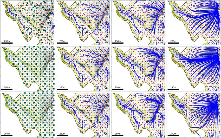
bioRxiv preprint first posted online Oct. 10, 2018; doi: http://dx.doi.org/10.1101/440420. The copyright holder for this preprint
(which was not peer-reviewed) is the author/funder, who has granted bioRxiv a license to display the preprint in perpetuity.
                                  It is made available under a CC-BY 4.0 International license.

         an individual level (e.g. cell/organism tracking), a natural approach is to model an individual’s
         movement as a velocity-jump random walk (VJRW) [32]. In a VJRW, an individual undergoes an
         alternating sequence of smooth “runs” with constant velocity and “turns” where a new velocity is
         chosen. We note that the latter provides a point for including orientation. In a groundbreaking
         paper, Patlak [37] derived a governing partial differential equation (PDE) for motions of this form,
         a model of advection-diffusion type in which an external bias drifts the population in a specific
         direction. This model foreshadowed phenomenological models such as the well-known Keller-Segel
         [22] model for chemotactic guidance, a popular choice for incorporating taxis-type orientation into
         models for biological movement [35].

             Many models implicitly assume that guidance information is local to the individual’s position.
         For an adult fruitfly, capable of detecting and orienting according to a (spatial) chemical gradient
         computed across its antennae [6], the length scale of antenna separation is microscopic in com-
         parison to its movement in the landscape at large. The scale of gradient detection is, effectively,
         local. Yet in other cases the sampling region for cue detection may be much larger, covering a
         significant portion of the individual’s environs. An obvious example lies in visual sensing, where
         individuals can assess information within eyesight. Here, the perceptual range – the “distance from
         which a particular landscape element can be perceived as such (or detected) by a given animal”
         [24] – is a key concept and has been estimated at distances ranging from metres to kilometres,
         according to species, habitat and conditions [54, 43, 30, 51, 11, 46, 12]. Auditory cues are also
         detectable at a distance: a few kilometres for elephants [26] and possibly hundreds of kilometres
         for baleen whales [38], the latter possible via the properties of sound propagation in water. Less
         obviously, fish and amphibians detect the electric fields generated by nearby organisms and objects,
         a process termed electrolocation [20]. Long-range assessments can also extend down to the single
         cell, with certain cells generating membrane protrusions (filopodia, cytonemes) that stretch mul-
         tiple cell diameters to acquire inherently nonlocal information about their tissue landscape [50, 23].

             In this paper we explore models, founded on a simplified VJRW, that incorporate local and
         nonlocal evaluation of the environment. Orientation enters by biasing turns into certain directions,
         according to an underlying navigation field that can be adapted to account for various modes of
         sampling the environment. As prototype models we consider three simple responses to a scalar
         cue: a local gradient-based orientation, a nonlocal gradient-based orientation and a nonlocal re-
         sponse in which orientation is according to the maximum cue value over the perceptual range.
         The corresponding macroscopic models for the VJRW are of drift-anisotropic diffusion type. Via
         approximating expansions, we show how the simple local gradient model reduces to a Keller-Segel
         equation while the nonlocal models reduce to forms related to commonly-employed integro-PDE
         equations, such as those used to describe nonlocal chemotaxis responses [17], cell interactions [36],
         swarming/flocking [28] and, pertinently, information gathering over some perceptual range [10].
         While these simplified forms strictly apply only when the orientation is weak, higher order approx-
         imations can extend the range of application. Separate approximations can be applied for very
         strong orientation responses, generating a pure drift equation in the simplest case.

            To demonstrate how nonlocal assessment contributes to population structuring, we consider a
         specific case-study application: hilltopping in butterflies, moths and other insects. In hilltopping,
         population members move up slope and localise at peaks and summits, a “lekking” behaviour
         that increases mating encounters [48, 47, 1]. Given that elevation is (primarily) sensed visually,
         we explore how perceptual range and assessment mode impacts on the macroscopic population
         movement. Gradually introducing noise into an idealised elevation profile, we show how nonlocal
         responses can allow a population to overcome roughness. Using terrain data for the Bodega

                                                                       2
bioRxiv preprint first posted online Oct. 10, 2018; doi: http://dx.doi.org/10.1101/440420. The copyright holder for this preprint
(which was not peer-reviewed) is the author/funder, who has granted bioRxiv a license to display the preprint in perpetuity.
                                  It is made available under a CC-BY 4.0 International license.

         Marine Reserve, a recent site of field studies [15], these findings are shown to extend to natural
         environments, with nonlocal sampling allowing the population to accumulate on a select subset
         of prominent peaks. We discuss the results both generally and within the specific context of
         hilltopping.

         2. Model framework

         We first outline the framework, referring to [32, 45, 18, 52] for further details. We let t denote time,
         x ∈ Rl the spatial coordinate and v ∈ Rl the velocity. While the following derivation is general,
         in this work we focus on two-dimensional navigation (l = 2). This type of navigation is relevant
         for movement across a landscape. Individuals move via a VJRW with instantaneous waiting time
         between reorientations, requiring two probability distributions: a runtime distribution over R+
         that dictates the reorientation rate and a turning distribution over velocity space V that describes
         the new velocity. The former is taken to be a standard Poisson process, that is, exponentially
         distributed runtimes with constant mean runtime τ (or turning rate λ = 1/τ ). We note that other
         choices of runtime can be made, potentially giving rise to subdiffusive or superdiffusive behaviour
         [13, 49, 9]. For the turning distribution we assume: (i) individuals move with a fixed speed s
         (i.e. v = sSl−1 ,); (ii) the new heading does not depend on the previous heading. Assumption (i)
         means that the turning distribution can be defined in terms of a directional distribution on the
         unit sphere, q(n|t, x), specifying the probability of choosing direction n ∈ Sl−1 following a turn,
         where n is the directional heading on the unit sphere Sl−1 .

             For the above VJRW, given stochastically independent walkers, we can obtain an evolution
         equation for the macroscopic population density at position x and time t, u(x, t). The process
         is to first write down the analogous transport (or kinetic) equation and, via scaling, obtain a
         macroscopic equation in an appropriate limit. We refer to [18] (and references therein) for details
         and simply state that applying a moment closure method1 generates a macroscopic model in the
         form of the Drift-Anisotropic Diffusion (DAD) equation

                                      u(t, x)t + ∇ · (a(t, x)u(t, x)) = ∇∇ : (D(t, x)u(t, x)).                                      (1)

         In the above, D(t, x) is a l × l diffusion tensor matrix and a(t, x) is the l-dimensional advection
         velocity. The colon (:) denotes the contraction of two tensors, resulting in a summation across all
         second order derivatives
                                                             l
                                                           X     ∂ ∂Du
                                               ∇∇ : Du =                .
                                                          i,j=1
                                                                ∂xi ∂xj

         The macroscopic quantities a and D are determined from the statistical properties of the individual-
         level model: mean speed, mean runtime and the turning distribution. Specifically,
                                               Z
                                a(t, x) = s           nq(n|t, x)dn ,                                      (2)
                                                  l−1
                                               ZS
                                D(t, x) = τ           (sn − a)(sn − a)T q(n|t, x)dn .                     (3)
                                                            Sl−1

            1 Our moment closure relies on two frequently used assumptions: (i) the population’s variance is computable

         from the equilibrium distribution, and (ii) a fast flux relaxation. The latter effectively states that, at the space/time
         scales of interest, the particle responds instantaneously to the information obtained at its current position. In
         later simulations we compare directly the distributions from repeated simulations of the stochastic model and the
         macroscopic model, confirming their validity for the present problem.

                                                                       3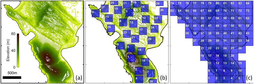
bioRxiv preprint first posted online Oct. 10, 2018; doi: http://dx.doi.org/10.1101/440420. The copyright holder for this preprint
(which was not peer-reviewed) is the author/funder, who has granted bioRxiv a license to display the preprint in perpetuity.
                                  It is made available under a CC-BY 4.0 International license.

         Thus, the drift is proportional to the expectation of q and the anisotropic diffusion is proportional
         to its variance-covariance matrix.

            Environmental guidance is encoded in q, via biasing turns into specific directions. For the
         two-dimensional case considered here, the von Mises distribution [25] is a natural choice:
                                                                           1
                                                        q(n | k, ν) =            ekn·ν ,                                            (4)
                                                                        2πI0 (k)

         where Ij (k) denotes the modified Bessel function of first kind of order j. Equation (4) plays an
         analogous role to the normal distribution of linear statistics, and generates a predominance of
         turns into preferred direction ν ∈ S1 with certainty increasing with concentration parameter k. We
         note that ν(x, t) and k(x, t) are functions of space and time to reflect variation in the direction
         and strength of the orienteering cue, but we omit the dependences for clarity of presentation. As
         k → 0, q tends to a uniform distribution, while as k → ∞, q approaches a singular distribution in
         which the preferred direction is always selected.

            Expectations and variance-covariance matrices of (4) can be explicitly calculated [19], yielding
         the following drift-velocity and diffusion tensor

                                                      I1 (k)
                                        a(k, φ) = s          ν,                                                                     (5)
                                                      I0 (k)
                                                     τ s2                           I1 (k)2

                                                                I2 (k)          2             I2 (k)
                                        D(k, φ) =           1−           I − τs             −          A.                           (6)
                                                      2         I0 (k)              I0 (k)2   I0 (k)

         Intuitively, the drift is in the dominant direction. The anisotropic diffusion tensor has been decom-
         posed into isotropic (proportional to the identity matrix I) and anisotropic (proportional to the
         singular matrix A = νν T ) components. The relative strength of diffusion to advection depends on
         k, via the modified Bessel functions. We note that
                 I1 (k) I2 (k)
             •   I0 (k) , I0 (k)   → 0 as k → 0 and we converge to isotropic diffusion;
                 I1 (k) I2 (k)
             •   I0 (k) , I0 (k)   → 1 as k → ∞ and we converge to a pure-drift equation;
                 I1 (k)2       I2 (k)
             •   I0 (k)2   >   I0 (k)   for all k, and hence the dominating axis of diffusion lies orthogonal to that of
                 drift.
         Modified Bessel functions arise in numerous applications and a correspondingly large literature has
         emerged [31]. In particular, approximating expansions are available for small and large arguments,
         as presented in Appendix A.

         3. Orientation: local and nonlocal sampling

         Orienteering information is encoded into a navigation vector field, denoted w(x, t) ∈ Rl . The
                                                                                                       w(x,t)
         directions and vector lengths of w form the inputs for the von Mises distribution: ν(x, t) = |w(x,t)|
         and k(x, t) = |w(x, t)|. The navigation field in turn depends on a navigating factor, represented as
         a single scalar intensity function E(x, t), such as chemical concentration, elevation, temperature
         or magnetic intensity. We define w to have one of two generic forms:
             • Local sampling – the navigation field is computed according to information obtained strictly
               at an individual’s current position;

                                                                        4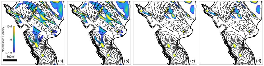
bioRxiv preprint first posted online Oct. 10, 2018; doi: http://dx.doi.org/10.1101/440420. The copyright holder for this preprint
(which was not peer-reviewed) is the author/funder, who has granted bioRxiv a license to display the preprint in perpetuity.
                                  It is made available under a CC-BY 4.0 International license.

         Figure 1: (a-c) Illustration of (M1)-(M3) in the context of hilltopping behaviour. Red circles and blue stars indicate
         starting and expected final locations of the individual; green arrows represent the initial direction of the bias; red
         and blue lines indicate the sampling region at the start and at the end of movement. (a) Local slope response; (b)
         Individual responds to the elevation angle, with θR > θL implying a bias to the right; (c) Individual responds to the
         absolute elevation, with EL > ER implying a bias to the left. (d) Illustration of nonlocal sampling. An individual
         at x samples the environmental cue E at points within some compact region (here taken to be a circle centred on
         x and characterised by the perceptual range, R), averaging the response into a preferred directional bias (green
         arrow).

             • Nonlocal sampling – the navigation field is computed over some spatially-extended sampling
               region, centred on the current position.
            For both sampling mechanisms we consider a general form before tailoring into the following
         three model prototypes:
         (M1) a local and linear gradient model;
         (M2) a nonlocal and nonlinear gradient model;
         (M3) a nonlocal and nonlinear maximum model.
         The above have widespread applicability, but are particularly intuitive in the context of hilltopping.
         In (M1), responses are to the local gradient, as highlighted in Figure 1(a). An individual, initially
         at the red circle, moves up the slope until coming to rest at the nearest local peak (blue star).
         In (M2), presented in Figure 1(b), evaluations are made up to a given perceptual range (red/blue
         lines). The bias is weighted in the direction of the maximum elevation angle from the current
         position and, while all three peaks are observed from its initial position, the individual typically
         moves towards the closer of the two higher peaks: despite its lower overall height, it has the larger
         elevation angle from the initial location. In (M3), the individual estimates the true height of peaks
         and biases according to the highest peak within perceptual range, as highlighted by the schematic
         in Figure 1(c).

         3.1. Local sampling
         Local models implicitly assume pointwise sampling (at the scale of the overall environment). To
         generate a directional response we assume the local gradient of E can be determined. This results
         in a (local) tropotaxis response in which w points in the direction of ∇E and the magnitude

                                                                       5
bioRxiv preprint first posted online Oct. 10, 2018; doi: http://dx.doi.org/10.1101/440420. The copyright holder for this preprint
(which was not peer-reviewed) is the author/funder, who has granted bioRxiv a license to display the preprint in perpetuity.
                                  It is made available under a CC-BY 4.0 International license.

         depends on E and |∇E| (and other factors, if necessary). Thus,

                                                                                  ∇E
                                                      w(x, t) = k(E, |∇E|)            .
                                                                                 |∇E|

         where k(E, |∇E|) describes the strength and form of response: positive (negative) values of k imply
         attraction (repulsion). We note that k(E, |∇E|) must satisfy k = 0 for |∇E| = 0. Given data, k
         can be estimated through fitting, for example in leukocyte chemotaxis where chemokine responses
         have been calculated for different concentrations and gradients [21].

             To generate the prototype model (M1) we invoke the simple choice of linear gradient depen-
         dence: k = κ1 |∇E| with associated response coefficient κ1 . The navigation field is therefore
         directly proportional to ∇E, yielding
                                                 w = κ1 ∇E .                                      (M1)
         We remark that similar models have been proposed in a cell biology context, where E arises from
         local crowding between cells [3]. Movement in these models can either be repulsive and hence
         proportional to −∇E, or attractive and hence proportional to ∇E [3]. We note that such models
         consider navigation based from interactions between individuals, whereas we focus on processes
         where individuals do not interact with each other. Instead, navigation information is obtained
         from an underlying environmental cue.

         3.2. Nonlocal sampling
         We consider the schematic in Figure 1(d) and suppose an individual at x computes a movement
         response by directly sampling the environment at positions x + ri for i = 1 . . . L, where L is
         total number of perceived locations. Sampling could occur through (for an organism) visual focus
         on a distant point or (for a cell) extending a filopodium. We define a probability distribution,
         Ω(r|x, t), that denotes the probability that position x + r is sampled from position x at the time
         of reorientation t. Logically, Ω has compact support to reflect a maximum perceptual range, but
         analytically convenient forms with decaying tails (such as Gaussians) may also be reasonable. We
         suppose the strength of attraction towards (or repulsion from) x + r is encoded into a response
         function g(E(x+r, t), E(x, t), |r|), potentially depending on the cue at both the current and sampled
         points, as well as the sampling distance. The attraction vector pr (x, t) in direction r/ |r| due to
         information at x + r is hence
                                                                                                r
                                            pr (x, t) = Ω(r)g(E(x + r, t), E(x, t), |r|)           .
                                                                                               |r|

         We suppose w is formed from the net attraction, obtained by sampling over different locations and
         calculating the average. Thus, we take
                                                       L
                                                   1X                                          r
                                     w(x, t) =           Ω(r|x, t)g(E(x + r, t), E(x, t), |r|) .
                                                   L i=1                                      |r|

         If a large number of points are sampled we can approximate w via the integral form
                                          Z
                                                                                     r
                               w(x, t) =       Ω(r|x, t)g(E(x + r, t), E(x, t), |r|) dr .                                           (7)
                                           R l                                      |r|

         This generic formulation is easily adapted and we next consider the simple prototype models. Note
         that here, for simplicity, we exclusively concentrate on uniform sampling over a circular region of

                                                                       6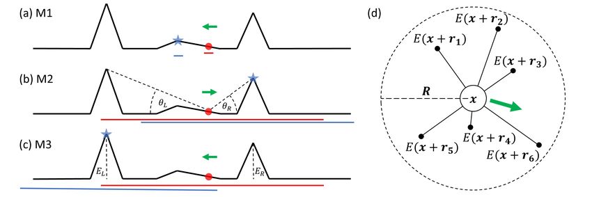
bioRxiv preprint first posted online Oct. 10, 2018; doi: http://dx.doi.org/10.1101/440420. The copyright holder for this preprint
(which was not peer-reviewed) is the author/funder, who has granted bioRxiv a license to display the preprint in perpetuity.
                                  It is made available under a CC-BY 4.0 International license.

         radius R, where we define R to be the perceptual range
                                                    1
                                                      VR   if r ∈ BR (0)
                                       Ω(r|x, t) =                       ,                                                          (8)
                                                       0 otherwise

         where BR (0) is the ball of radius R, centred on the origin, and VR is its volume (i.e. VR = πR2
         for l = 2).

         3.2.1. Nonlocal gradient sampling
         Suppose attraction is according to the nonlocal gradient of E

                                                                              E(x + r, t) − E(x, t)
                                      g(E(x + r, t), E(x, t), |r|) = κ2                             ,
                                                                                       |r|

         with sensitivity coefficient κ2 . Substituting both the above and (8) into (7), we obtain
                                                        Z
                                                    κ2        E(x + r, t) r
                                          w(x, t) =                          dr .
                                                    VR BR (0)     |r|    |r|

         Notably, a Taylor series expansion about x applied to the RHS yields
                                                                      κ2
                                                      w(x, t) =          ∇E + O(R2 ) .
                                                                      2
         Hence, as R → 0 the nonlocal gradient model converges to the local gradient model with κ2 = 2κ1 .

             It is straightforward to incorporate nonlinear processing of the cue, and in particular we consider

                                                                            E(x + r, t)n − E(x, t)n
                                      g(E(x + r, t), E(x, t), |r|) ∝                                .
                                                                                      |r|

         The parameter n gives additional control, increasing the weighting of attraction bias as n is in-
         creased. This gives the following navigation field (M2)

                                                            E(x + r, t)n r
                                                    Z
                                       w(x, t) = α2                          dr .                   (M2)
                                                     BR (0)     |r|      |r|
                                                                                       κ2 ω1
         We note that we have absorbed various constants into α2 =                           , where
                                                                                       VR ωn

                                                                      E(x + r, t)i r
                                                           Z
                                                   ωi =                                dr .
                                                             BR (0)       |r|      |r|

         The scaling normalises the navigation field, so that the magnitude remains essentially the same as
         n is altered. Note that Taylor expansion again yields (M1) in a small R approximation.

         3.2.2. Maximum value evaluation
         Our second prototype nonlocal model takes g to depend on the absolute size of the cue at E(x+r, t)

                                             g(E(x + r, t), E(x, t), |r|) = κ3 E(x + r, t) ,

                                                                        7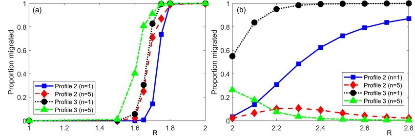
bioRxiv preprint first posted online Oct. 10, 2018; doi: http://dx.doi.org/10.1101/440420. The copyright holder for this preprint
(which was not peer-reviewed) is the author/funder, who has granted bioRxiv a license to display the preprint in perpetuity.
                                  It is made available under a CC-BY 4.0 International license.

         where κ3 is the sensitivity coefficient. Substituting into (7) along with (8) now yields
                                                       Z
                                                    κ3                     r
                                        w(x, t) =             E(x + r, t) dr .
                                                    VR BR (0)             |r|

         The distinction with the gradient-based evaluation is exemplified through a Taylor expansion,
         where we find
                                          w(x, t) = κ3 R∇E + O(R3 ) .
         Hence, as R → 0 the navigation vector field shrinks to zero length and orienteering information is
         lost. As before, we can extend to a nonlinear form to obtain (M3)
                                                    Z
                                                                         r
                                       w(x, t) = α3         E(x + r, t)n dr,                         (M3)
                                                     BR (0)             |r|
                         κ3 ω1
         where α3 =            and
                         VR ωn
                                                           Z
                                                                                      r
                                                    ωi =              E(x + r, t)i       dr ,
                                                             BR (0)                  |r|
         provides the normalisation as n is altered.

         4. Approximations

         A choice must be made about whether to perform direct stochastic simulations of the VJRW
         model or solve the full DAD model (1) with their Bessel function dependent coefficients (5)-(6).
         Both approaches have associated costs. Simulations of the stochastic VJRW are expensive, scaling
         with population size; evaluations of the modified Bessel functions and implementing anisotropic
         diffusion terms are also costly. In an analytic context, anisotropic diffusion terms may be more
         difficult to deal with than isotropic counterparts. Consequently, it is worthwhile investigating
         simplifying reductions.

         4.1. Local sampling approximations
         We consider model (M1). Expansions of the modified Bessel functions (see Appendix A) allow
         a series of approximations to (1) to be obtained, relevant for small or large values of k (weak or
         strong navigating cues, respectively). For weak cues the lowest order approximation (O(k 1 )) yields
         the well known Keller-Segel equation for (chemo)taxis

                                                       ut = d∇2 u − ∇ · (χu∇E) ,                                                    (9)

         with constant diffusion (d = τ s2 /2) and chemotactic (χ = sκ1 /2) coefficients2 . The above is
         strictly valid only for weak cues, but a series of higher order “corrections” extends the range of
         k values for which the approximation accurately describes the full DAD model. We tabulate up

           2 We remark the general choice k would instead yield a general form Keller-Segel equation in the first order

         approximation:
                                                                               E
                                        ut = d∇2 u − ∇ · k(E, ∇E, |∇E|)u∇           .
                                                                             |∇E|

                                                                        8
bioRxiv preprint first posted online Oct. 10, 2018; doi: http://dx.doi.org/10.1101/440420. The copyright holder for this preprint
(which was not peer-reviewed) is the author/funder, who has granted bioRxiv a license to display the preprint in perpetuity.
It is made available under a CC-BY 4.0 International license.
to O(k 4 ) in Appendix B. For example, the O(k 2 ) approximation in two dimensions introduces a
correction for each of the diffusion and chemotaxis terms, such that
! ! !
2 2 2
κ21 |∇E| κ21 |∇E| κ21 |∇E|
ut = D∇∇ : 1− 2 I−2 2 − 2 A u
8 + 2κ21 |∇E| 4 + 2κ21 |∇E| 8 + 2κ21 |∇E|
! !
2
2 + κ21 |∇E|
−∇· χ 1− 2 u∇E . (10)
4 + κ21 |∇E|
Notably, this correction introduces the anisotropic diffusion component. We remark that diffusion
coefficients remain positive for all κ1 , so the system is well-behaved.
As k becomes larger the approximations become less useful: more terms are required to achieve
reasonable accuracy, and it would be natural to instead revert to the full DAD model (1). However,
very large k can alternatively be dealt with through large argument approximations (Appendix B).
For example, for sufficiently large k (corresponding to strong navigation fields) we can approximate
the full DAD model (1) via the pure drift-equation
s
ut + ∇ · u∇E = 0 ,
|∇E|
which simply generates direct movement with speed s in the direction of the steepest gradient. Cor-
rections to this again yield a sequence of chemotaxis/anisotropic diffusion style models, tabulated
in Appendix B. For example, the O(k −1 ) approximation in 2D generates
τ s2
1 s 2κ1 |∇E| − 1
ut = ∇∇ : (I − A)u − ∇ · u∇E .
κ1 |∇E| |∇E| 2κ1 |∇E|
The anisotropic diffusion in the above corresponds to a degenerate/singular form in which diffusion
is one-dimensional and along the axis orthogonal to the preferred direction.
4.2. Nonlocal sampling approximations
The process is identical for nonlocal sampling scenarios, and we therefore only state the first order
weak cue form for the general navigation field (7), and for both (M2)-(M3). In the general case,
the first order approximation under a weak cue yields a nonlocal integro-PDE equation
Z
r
ut = d∇2 u − ∇ · σu Ω(r|x, t)g(E(x + r, t), E(x, t), |r|) dr , (11)
Rl |r|
for d = τ s2 /2 and σ = s/2. The above is closely related to various nonlocal PDE models. For
example, if E is directly based on the population’s own density distribution the above is similar to
those employed to describe swarming [28] and cell interactions [36]. Moreover, the above is closely
related to the model proposed in [10] for perceived gradient following.
If we consider the two prototype models, the above becomes
!
E n (x + r, t) r
Z
2
ut = d∇ u − ∇ · σα2 u dr ,
BR (0) |r| |r|
9bioRxiv preprint first posted online Oct. 10, 2018; doi: http://dx.doi.org/10.1101/440420. The copyright holder for this preprint
(which was not peer-reviewed) is the author/funder, who has granted bioRxiv a license to display the preprint in perpetuity.
It is made available under a CC-BY 4.0 International license.
Profile One (a) Profile Two (b) Profile Three (c) Profile Four (d)
1 2 30
1
E(y) E(y) E(y) E(y)
0 0 0 0
0 y 2 0 y 6 0 y 6 0 y 6
Figure 2: Four different idealised elevation profiles.
for (M2), and !
Z
r
ut = d∇2 u − ∇ · σα3 u E n (x + r, t) dr ,
BR (0) |r|
for (M3).
4.3. Numerical validation
We restrict our validation to local gradient sampling under an environmental cue that does not
vary with time. The population is initially distributed uniformly across the rectangular region
0 ≤ x ≤ 1, 0 ≤ y ≤ 2. We generate a quasi-one-dimensional scenario by assuming the cue varies
only with y, specifically
2
E(y) = e−β(y−1) . (12)
The corresponding cue profile is presented in Figure 2(a). The dominant direction for individuals
with locations y < 1 (y > 1) will be π/2 (−π/2) and subsequently individuals are expected ac-
cumulate along the ridgeline y = 1. Comparisons are presented for (i) the average behaviour of
multiple realisations of the velocity-jump process, (ii) numerical solution of the full DAD model
(1) under (5)-(6), and (iii) the O(k) to O(k 4 ) approximations. These approximations rely on an
assumption that the strength of the navigating cue, k, is small. Numerical methods are described
in the Supplementary Materials, Section S3. Briefly, an implicit timestep method and an operator
splitting method are used to numerically solve the full DAD model and the corresponding O(k) to
O(k 4 ) approximations. The trajectories of individuals in the velocity-jump process are simulated
directly as described in [34], and additionally detailed in the Supplementary Material, Section S3.
The Bessel function approximations are independent of s and we therefore expect that the
difference between approximations and the full DAD model (1) is constant as s changes. Thus,
differences between solutions under increasing s should stem only from the assumptions made
when deriving the macroscopic model from the velocity-jump process. The difference between the
approximations and either the full DAD model solution or the average behaviour of the velocity-
jump process decreases with the order of the approximation. Further, both the full DAD model
solution and approximations prove to be less accurate against the average velocity-jump behaviour
as s increases (Supplementary Material, Section S1), consistent with previous investigations [34].
Generally, whether (1) provides a reasonable description of the underlying random walk depends
on whether the spatial and temporal scales are appropriately macroscopic, for example see [5, 18]
for further discussion. Specifically, average run lengths need to be short, compared to the overall
domain dimensions, and individuals need to make numerous turns over the study time.
10bioRxiv preprint first posted online Oct. 10, 2018; doi: http://dx.doi.org/10.1101/440420. The copyright holder for this preprint
(which was not peer-reviewed) is the author/funder, who has granted bioRxiv a license to display the preprint in perpetuity.
It is made available under a CC-BY 4.0 International license.
We next explore the match for fixed s = 0.001 and varying response coefficient κ1 . Vary-
ing κ1 directly influences the concentration parameter k, so increasing κ1 should impact on the
matching ability of the approximations. Note that for a quasi-one-dimensional case the diffusion
tensor reduces to a function depending on y and k, denoted d(y), while the drift reduces to a
“chemotaxis”-type function, denoted a(y). As expected, truncating at higher order terms yields
a better fit for these functions, see Figures 3(a,d,g) for a(y) and Figures 3(b,e,h) for d(y). For
sufficiently small κ1 (e.g. κ1 = 0.5) even the lowest order approximations prove highly acceptable,
while larger values (e.g. κ1 = 2) demand a higher order for a good fit.
Turning to full numerical solutions, we compare O(k) to O(k 4 ) approximations with those of
the full DAD model and the average velocity-jump behaviour. Note that for the parameter values
under consideration, the full DAD model closely describes the average velocity-jump behaviour.
For κ1 = 0.5, Figure 3(c), all approximations are generally successful, although O(k) and O(k 2 )
approximations show some inaccuracy in regions where the diffusivity function approximation is
at its worst. Increasing κ1 generates a poorer fit: under this cue distribution and κ1 = 2, the
maximum value of k ≈ 5.43 is beyond the expected range of k values for reasonably valid approx-
imations. Nevertheless, the O(k 4 ) still proves reasonably accurate.
Overall, numerical comparisons validate the approximations, but only when k remains within
relevant regions. Thus, if it is known that a particular cue provides only a weak bias (say, a
cell migrating in a fairly stable and shallow gradient) it is reasonable to use the simplified PDE,
such as the local or nonlocal Keller-Segel equation. If, rather, cue strength cue varies widely, one
should resort to employing the full DAD equation (1), assuming the spatial/temporal scales are
appropriately macroscopic.
5. Short and long-range sampling: hilltopping case study
The accumulation of butterflies, moths and other insects at hilltops has been widely documented
[48, 47, 8, 1, 43, 15]. Many insect populations fluctuate over different locations and seasons, and
strategies that offer robustness against extinction events are necessary. Hilltopping is perceived
as one such mechanism, due to an improved rate of mating encounters. The relatively local scale
over which movements occur, the precision to which terrain can be documented and the (relative)
ease of tracking/counting population members combine to form an ideal system for determining
how environments structure a population. Given visual assessment of topography, it is natural
to query how perceptual range impacts on hilltopping. Natural terrains are typically “rough”, so
responses based strictly on the local gradient could easily trap a large percentage of the population,
scattered through small accumulations on many local peaks. Instead, studies of a hilltopping but-
terfly (Melitaea trivia) indicate that their orientation may be according to both the local slope and
higher peaks within a longer range (∼50 metres) [43]. Moreover, a recent capture-mark-recapture
study of the tiger moth (Arctia virginalis) revealed that populations accumulated only on a subset
of summits, with the largest numbers found at the highest elevations [15].
Motivated by these findings, we use this section to explore how short- and long-range topo-
graphical sensing alters hilltopping outcomes. We consider our three prototype models for moving
up slopes, effectively describing populations that respond to: (M1) the strictly local gradient; (M2)
the nonlocal gradient, that is, according to the elevation angle of terrain within perceptual range;
(M3) the true height of land within perceptual range. We first generate idealised terrains in order
to test principles before considering an application using elevation data for the Bodega Marine
Reserve, as used in a recent hilltopping survey conducted by Grof-Tisza et al. [15].
11bioRxiv preprint first posted online Oct. 10, 2018; doi: http://dx.doi.org/10.1101/440420. The copyright holder for this preprint
(which was not peer-reviewed) is the author/funder, who has granted bioRxiv a license to display the preprint in perpetuity.
It is made available under a CC-BY 4.0 International license.
Profile One
(a) (b) (c)
3 0.6 2
κ1 = 0.5 a(y) d(y) U(y)
-3 0 0
0 y 2 0 y 2 0 y 2
(d) (e) (f )
3 0.6 4 4
κ1 = 1.0 a(y) d(y) U(y)
-3 0 0 0
0 y 2 0 y 2 0 y 2
(g) (h) (i)
3 0.6 8
κ1 = 2.0 a(y) d(y) U(y)
-3 0 0
0 y 2 0 y 2 0 y 2
Figure 3: (a),(d),(g) Comparison between the drift-velocity function (red), and the corresponding O(k) to O(k4 )
approximations (orange, purple, green, blue, respectively) for (a) κ1 = 0.5, (d) κ1 = 1, (g) κ1 = 2. (b),(e),(h)
Comparison between the diffusivity function (red), and the corresponding O(k) to O(k4 ) approximations (orange,
purple, green, blue, respectively) for (b) κ1 = 0.5, (e) κ1 = 1, (h) κ1 = 2. (c),(f),(i) Comparison of the average
velocity-jump behaviour (black, dashed), and the numerical solutions to the full DAD model (red) and the O(k)
to O(k4 ) approximations (orange, purple, green, blue, respectively) for (c) κ1 = 0.5, (f) κ1 = 1, (i) κ1 = 2.
Random walk parameters are set at s = 0.001 and τ = 1; elevation is set by (12) with β = 10; simulations are
based on averaging over 106 realisations of the VJRW and a spatial discretisation of ∆y = 0.001 for the numerical
approximation of the continuous models. Simulations are computed until tend = 100.
12bioRxiv preprint first posted online Oct. 10, 2018; doi: http://dx.doi.org/10.1101/440420. The copyright holder for this preprint
(which was not peer-reviewed) is the author/funder, who has granted bioRxiv a license to display the preprint in perpetuity.
It is made available under a CC-BY 4.0 International license.
We note that several previous simulation studies have explored hilltopping. For example, in [41,
39] an agent-based modelling approach was used to simulate butterfly movement paths, based on
field study data [43]. Topography was shown to channel movement paths along “virtual corridors”.
Further agent-based studies in [42] highlighted the importance of an element of randomness in the
movement paths to avoid the above described trapping. In [34] the multiscale framework used here
was employed to demonstrated how accumulations formed by hilltopping could optimise mating
for low-density populations, but may be disadvantageous for more abundant populations. The
current study here extends that work, specifically incorporating long-range perception to explore
its impact on population distribution.
5.1. Idealised study
We first explore how the prototype orienteering mechanisms impact hilltopping in a series of
idealised studies. We assume a quasi one-dimensional terrain and, unless stated otherwise, initially
suppose the population to be uniformly randomly distributed across the terrain. We first examine
the suitability of models (M1)-(M3) to describe hilltopping, considering movement on a terrain
containing a single peak centred at y = 1, as presented in Figure 2(a). For succinctness we simply
note that all model prototypes allow the population to relocate to the peak by t = 100; results and
further discussion are provided in the Supplementary Material, Section S2.1. Thus, all proposed
mechanisms are plausible and we shift to a more sophisticated analysis of the mechanisms.
5.1.1. Perceptual range and nonlocal response order
Here we investigate the influence of the perceptual range, R, and nonlocal response order, n. We
consider a landscape containing two peaks of different heights, as highlighted in Figure 2(b). For
model (M3) we observe a significant change between R = 1.5 and R = 2.0. For smaller radii the
population is split into separated sub-populations, one on each hilltop with the majority of the
individuals on the higher of the two peaks. In contrast, for R = 2.0 the individuals merge into a
single contiguous population at the higher peak. Comparing the dominant direction for the two
radii, Figure 4(c) and (f), a transition is observed such that under smaller radii each peak has
its own “zone of attraction”. For larger radii, however, the zone of attraction for the larger peak
expands to cover the entire domain. Note that for this example, n does not qualitatively change
the results.
Under model (M2) with a high nonlocal order (n = 5), two distinct sub-populations are main-
tained even for large R. That is, even when the higher peak is fully within perceptual range of
members on the lower peak, the two sub-populations remain separate. Here, higher weighting is
applied according to the largest elevation angles. Consequently, the lower peak can always be
perceived as more attractive for individuals located sufficiently close. As the nonlinear order is
decreased, however, the sub-population that initially formed on the lower peak begins to migrate
towards the higher peak. This is reflected in the comparison of the dominant direction, Figure
4(l), where we observe a collapse from two zones of attraction to one. As the nonlocal gradient
model effectively places a weight on higher environmental cue values close to an individual, it is
difficult for an individual to move away from the peak if that weighting is further compounded by
a high nonlinear order.
To examine whether migration is unidirectional (from the lower to higher peak), we consider
the migration proportion for two initially separated populations: one uniformly distributed around
the lower peak and the second about the higher peak (see Supplementary Material, Section S2.1).
Notably, when peak to peak migration occurs it is only for those initially located on the lower
13bioRxiv preprint first posted online Oct. 10, 2018; doi: http://dx.doi.org/10.1101/440420. The copyright holder for this preprint
(which was not peer-reviewed) is the author/funder, who has granted bioRxiv a license to display the preprint in perpetuity.
It is made available under a CC-BY 4.0 International license.
Profile Two
Nonlocal maximum Nonlocal gradient
(a) (d) (g) (j)
25 25 30 30
R = 1.5 R = 2.0 R = 2.0 R = 2.5
t = 100 U(y) U(y) U(y) U(y)
0 0 0 0
0 y 6 0 y 6 0 y 6 0 y 6
(b) (e) (h) (k)
25 25 30 30
R = 1.5 R = 2.0 R = 2.0 R = 2.5
t = 1000 U(y) U(y) U(y) U(y)
0 0 0 0
0 y 6 0 y 6 0 y 6 0 y 6
n=1 (c) n=1 (f ) n=1 (i) n=1 (l)
Dominant Direction
Dominant Direction
Dominant Direction
Dominant Direction
n=5 n=5 n=5 n=5
0 y 6 0 y 6 0 y 6 0 y 6
Figure 4: Comparison of different R and n for the full DAD model (solid) and the average velocity-jump process
(dashed), respectively, using (a)-(f) (M3) and (g)-(l) (M2). Cyan/blue corresponds to n = 1, orange/black corre-
sponds to n = 5. Initially the population is uniformly distributed and the elevation profile corresponds to Profile
Two in Figure 2. Parameters used are as follows: (a)-(f) κ3 = 3, (g)-(l) κ2 = 0.3; random walk parameters are set
at τ = 1, s = 0.01; numerical simulations based on averaging over 2 × 10⁵ realisations of the VJRW and using a
spatial discretisation of ∆y = 0.001 for the numerical approximation of the continuous models.
Figure 5: Proportion of population initially located on the lower peak that migrates to the higher peak by t = 5000
for various R, n and peak height ratios. (a) Results for (M3), using κ3 = 3; (b) Results for (M2), using κ2 = 0.2.
Other parameters are set at ∆y = 0.003, τ = 1, s = 0.01.
14bioRxiv preprint first posted online Oct. 10, 2018; doi: http://dx.doi.org/10.1101/440420. The copyright holder for this preprint
(which was not peer-reviewed) is the author/funder, who has granted bioRxiv a license to display the preprint in perpetuity.
It is made available under a CC-BY 4.0 International license.
peak, which translocate to the higher one. We therefore investigate how the combination of per-
ceptual range, ratio of peak heights and nonlocal order influences the proportion of the lower peak
population that have migrated by a fixed time, set at t = 5000. The influence of peak height ratio
is determined via two elevation profiles, Figures 2(b)-(c), with peaks located at the same position
but with distinct heights to generate ratios of 1.5 and 2.0 respectively. Figure 5(a) summarises
the results for (M3). For all scenarios, there is negligible migration for R = 1 and full migration
by R = 2. In between, there is a steep transition with its location changing according to nonlocal
order and peak height ratio: increases in either will lower the perceptual range required to shift
the population. Effectively, an increase in either of these properties increase the attractiveness of
the higher peak and the population migrates accordingly. Figure 5(b) summarises the results for
(M2). Notably, there is now a significant difference between n = 1 and n = 5 for both profiles. As
discussed previously, the extra weighting toward higher environmental values close to an individ-
ual, introduced by the 1/|r| factor in the nonlocal gradient term, influences the dominant direction
(Figure 4(o)). Substantially altering the disparity between peak heights, though, can overcome
this additional weighting.
5.1.2. Influence of noisy environments
So far we have considered smoothly varying cues. In reality, environments are expected to be
considerably rougher, due to small-scale variations in topography. Since a strictly local response
depends on the gradient at a specific point, this variation may significantly impact on an individ-
ual’s ability to move across some environment. To explore this, we introduce a form of gradient
noise into our environmental cue: we refer to Appendix C for details, but remark that the added
noise contains local spatial correlation to ensure a differentiable underlying environment.
We examine the average displacement of a population moving in response to a linear topograph-
ical profile, Figure 2(d), subject to the addition of various levels of noise. Initially, the population
is uniformly distributed between y = 0 and y = 1.2 (and zero elsewhere). Average displacement
is calculated by numerically solving the full DAD equation (1) under twenty identically-prepared
noise terms. That is, we generate twenty different noise terms according to the same process,
with the only difference stemming from the numbers sampled from the (pseudo)-random number
generator. We then solve (1) for each of the noise terms and calculate the overall displacement
of the population, defined as the difference between the median of the population at t = 0 and
t = 500. We repeat this process for different levels of noise and scale according to the average
displacement under zero noise.
The results for models (M1)-(M3) are summarised in Figure 6 (a), where for the nonlocal mod-
els we consider R = 0.2, R = 0.5 and R = 1.0. As might be expected, increasing the strength of
the noise compared to the strength of the environmental cue results in a decrease in the average
displacement. Local sensing (M1) is the most susceptible to the added noise, with increasing noise
significantly reducing the displacement. Nonlocal models (M2)-(M3) prove considerably more re-
silient, particularly for large perceptual ranges. This result is intuitive, as the nonlocal response
involves averaging the environmental cue over the perceptual region, reducing the contribution of
any noise. Note that as R → 0 for (M2), we observe convergence to (M1), consistent with our
earlier findings. Overall, given that environments in nature are non-smooth and exhibit variation,
nonlocal responses may be necessary for successful migration.
We now return to the example with two peaks, with two initially distinct populations, and
examine how the presence of noise influences the successful migration from the lower to higher peak.
We note that a small amount of noise can elicit a large change in the proportion of the population
15bioRxiv preprint first posted online Oct. 10, 2018; doi: http://dx.doi.org/10.1101/440420. The copyright holder for this preprint
(which was not peer-reviewed) is the author/funder, who has granted bioRxiv a license to display the preprint in perpetuity.
It is made available under a CC-BY 4.0 International license.
Profile Two
(a) (b)
1 1
Migratory Proportion
Average displacement
M1
M2, R = 0.2
M2, R = 0.5
M2, R = 1.0 M2, R = 2.2
M3, R = 0.2 M2, R = 2.8
M3, R = 0.5 M3, R = 1.75
M3, R = 1.0 M3, R = 2.0
0.4 0
0 Noise Scaling 8 0 Noise Scaling 1
Figure 6: (a) Scaled average displacement by t = 500 for a population of individuals initially uniformly distributed
between y = 0 and y = 1.2 for both local (solid) and nonlocal (dashed) responses and three R values. For each
parameter combination the average displacement is obtained from 20 simulations on identically-generated terrain.
Parameters used are κ1 = 0.3, κ2 = 0.6, κ3 = 2.0, ∆y = 0.003, τ = 1, s = 0.01, n = 1. (b) Average proportion of
the population initially located on the lower peak in Profile Two that migrates to the higher peak by t = 5000 for
M3 and R = 1.75 (cyan), M3 and R = 2.0 (orange), M2 and R = 2.2 (green), and M2 and R = 2.8 (purple). For
each parameter combination the average migratory proportion is obtained from twenty simulations on identically-
generated terrain. Parameters used are κ2 = 0.6, κ3 = 1.5, ∆y = 0.003, τ = 1, s = 0.01, n = 1.
16bioRxiv preprint first posted online Oct. 10, 2018; doi: http://dx.doi.org/10.1101/440420. The copyright holder for this preprint
(which was not peer-reviewed) is the author/funder, who has granted bioRxiv a license to display the preprint in perpetuity.
It is made available under a CC-BY 4.0 International license.
Figure 7: (a) Topography of Bodega Marine Reserve study site. (b)-(c) Zones used for population counts, following
either (b) peak-centred or (c) tessellated gridding.
that undergoes migration (Supplementary Material, Section S2.1). To determine how different
levels of variation influence hilltopping, we append twenty identically-prepared noise terms to
Profile Two. Using two distinct R values we examine the proportion of individuals initially located
on the lower peak that migrate to the higher peak by t = 5000, presenting the results in Figure 6
(b) for (M2) and (M3). As expected, we find that increasing the amount of noise generally reduces
the ability for individuals to translocate to the higher peak for both models: for combinations of R
and κ that allow the entire population to relocate in the absence of noise, introducing noise inhibits
a portion of the population from doing so. Consistent with previous findings, larger perceptual
ranges offset noise-induced trapping. As naturally occurring environments do not typically exhibit
the smoothness of idealised models, this suggests that the mechanism by which sensory information
is processed must be able to account for the noise.
5.2. Bodega Marine Reserve study
5.2.1. Study site and elevation data
We extend our case study to a natural environment, utilising topographical data for the Bodega
Marine Reserve, a site of recent hilltopping studies [15]. High spatial resolution LIDAR data
was obtained from the United State Geological Survey’s “The National Map” project over the
co-ordinate range of the study site, and longitude, latitude, elevation and classification (water,
ground etc.) are extracted at each data point. Interpolation onto a regular grid is performed,
and the resulting topographical structure is mapped in Figure 7(a). This topographical structure
allows individuals to obtain navigation information in a manner that mimics the behaviour of a
population undergoing directed motion according to the topography in the Bodega Marine Re-
serve. A population of butterflies/moths is uniformly randomly distributed across the landmass
at t = 0 and their movements are followed over 20 hours. Of course, more realistic distributions
should account for oviposition/larval sites but a uniform distribution limits any subsequent bias
in the final distributions. Simulation methods are described in the Supplementary Methods. Note
that we impose boundary conditions that effectively confine the population within the bounds of
the region plotted in Figure 7(a), as described in the Supplementary Methods, Section S3.
For later analyses we subdivide the land region using two methods. The first is a peak-centred
scheme, Figure 7(b), where 200m by 200m (4 hectare) non-overlapping regions are defined accord-
ing to topography: (i) we find the complete set of local maxima; (ii) zone 1 is centred on the
17bioRxiv preprint first posted online Oct. 10, 2018; doi: http://dx.doi.org/10.1101/440420. The copyright holder for this preprint
(which was not peer-reviewed) is the author/funder, who has granted bioRxiv a license to display the preprint in perpetuity.
It is made available under a CC-BY 4.0 International license.
highest maximum and both this maximum and any others within distance are excluded; (iii) zone
2 is centred on the next highest non-excluded maximum and so forth. The second subdivision,
Figure 7(c), is a regular tessellation that intersects with the land coverage. The use of two methods
is to reduce bias due to zoning.
We consider the three prototype models for topographic sensing, (M1)-(M3). Note that in
order to concentrate on how altering the navigation field and its associated parameters impacts on
population structuring, we fix the speed, turning rate and sensitivity coefficients at values similar
to those in an earlier study [34]. Specifically, we set s = 4 m/min and a mean run time of τ = 1 min;
note that these values account for pauses/resting periods during flight. Sensitivity coefficients are
set at κ1 = 5, κ2 = 10 and κ3 = 0.2; the relationship between κ1 and κ2 ensures convergence
from (M2) to (M1) as R → 0; the relationship between κ2 and κ3 is to generate quasi-equaivalent
navigation fields for (M2) and (M3) when R = 50 m. To provide context to these values, a butterfly
located on a linear ramp of gradient 10% would choose an uphill direction on just over 75% of
occasions, rising to slightly more than 90% for a 20% gradient.
5.3. Navigation field variation
We first consider how orientation information changes as we shift from local to nonlocal models.
For ease of illustration we plot only a portion of the full study site (the top left region in Figure
7(a)). Plots are presented in the form of a “direction field”, where red arrows indicate the local
direction of w at selected points and blue lines indicate the trajectory traced out if an individual
exactly follows these arrows. Light blue circles indicate trajectory end points, and can be inter-
preted as attractors that potentially lead to local accumulations of the population.
The plots in Figure 8 show results for (M1), i.e. R = 0, and (M2) with R = 25, R = 100
and R = 500; note that these plots assume n = 5. Under local sampling we observe significant
fluctuations in arrow directions, with some arrows pointing in the direction of prominent peaks
but others directed elsewhere. Numerous local maxima exist, so that trajectories travel short dis-
tances before becoming trapped at an attractor. Transitioning to the nonlocal model, however,
dramatically reduces the number of attractors. The majority of trajectories now converge on a
select few summits (examples given by black arrowheads) and trajectories can be significantly
longer than the perceptual range. Effectively, movement is first according to the highest elevation
angle within range, but subsequent higher peaks may be observed. For example, in Figure 8 (c)
we see trajectories converging on the top-left attractor over a distance of approximately 1 km, an
order of magnitude greater than the perceptual range. Increasing R steadily reduces the num-
ber of attractors, such that by R = 500 all trajectories converge on one of just two attractors
within the plotted region, corresponding to prominent peaks. These peaks are not necessarily the
two highest peaks across the studied zone, rather they correspond to the highest within their region.
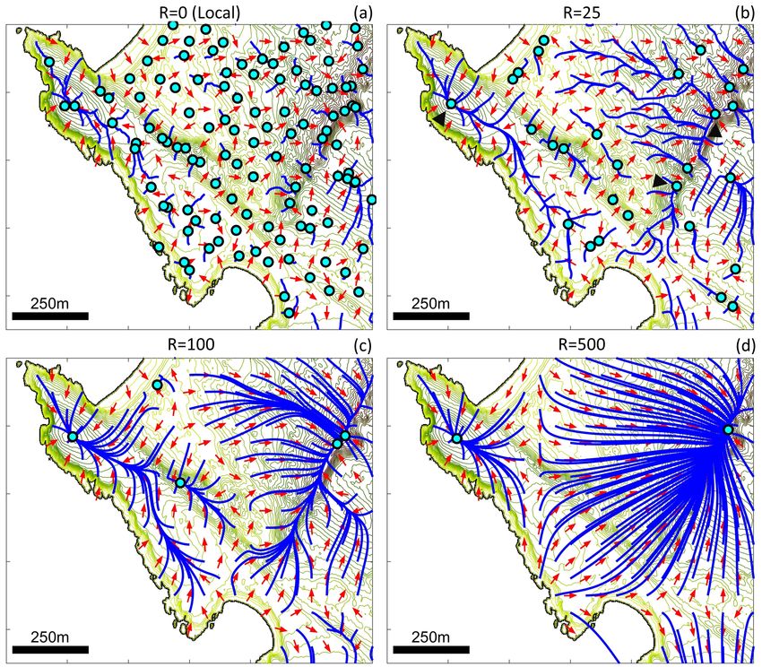
Further analyses have been performed for (M2) with n = 1 and (M3) with both n = 1 and
n = 5 (see Supplementary Materials, Section S2.2). Qualitatively we observe similar phenomena,
with a reduction in the number of attractors as R is increased. However, a few subtleties emerge:
(i) higher nonlocal orders promote the persistence of attractors at lower prominences, consistent
with our earlier idealised study; (ii) for n = 1, attractors can occasionally form some distance
away from the nearest local peak. This latter observation stems from the fact that, under a lower
nonlocal order, the weighting to summit points is diluted and evaluation is more according to a
broad assessment of the terrain. However, broadly the results are consistent and we note that
perceptual range, rather than the precise sensing model or degree of nonlinearity, appears to be
the primary determinant in the number of attractors. For the remainder of our investigation we
18bioRxiv preprint first posted online Oct. 10, 2018; doi: http://dx.doi.org/10.1101/440420. The copyright holder for this preprint
(which was not peer-reviewed) is the author/funder, who has granted bioRxiv a license to display the preprint in perpetuity.
It is made available under a CC-BY 4.0 International license.
Figure 8: Representation of orientation information, for w given by (M2) with (a) R = 0, (b) R = 25, (c) R = 100
and (d) R = 500. Note that the R = 0 case is effectively the local gradient model (M1). For these plots we use
n = 5 as the nonlinear coefficient.
therefore restrict to presenting the results for (M2) under n = 5, noting that results for the other
cases are qualitatively consistent.
5.4. Comparison of the velocity jump and macroscopic models
We proceed to simulate the VJRW and the full (unapproximated) macroscopic model (1) across a
range of R, using (M1), i.e. R = 0, and (M2) with R = 25, R = 100 and R = 500. Results are pre-
sented in Figure 9. Agent-based model simulations of the VJRW are presented in Figures 9(a)-(d),
where blue circles denote final locations (after 20 hours) and red dots indicate trajectories. The
results parallel the previous direction field plots. For the local model, some larger collections occur
at the most prominent peaks but the overall population remains scattered with numerous small
accumulations trapped at local maxima. Expanding the perceptual range reduces trapping, allow-
ing the population to coalesce into fewer and larger aggregates that correlate with the prominent
peaks. The capacity for long-range information to influence movement is particularly illustrated
by the individuals that move across the bays, attracted to peaks on the other side (arrowheads in
Figure 9(d)).
Under each agent-based simulation we show the corresponding population distributions pre-
dicted by the macroscopic model after 2, 8 and 20 hours. Note that the distributions correlate well
with those of the agent-based model, suggesting that the macroscopic model accurately captures
individual-level behaviour at the spatial and temporal scales of study. We subsequently focus on
19You can also read