Population Genomic Surveys for Six Rare Plant Species in San Diego County, California - Open-File Report 2018-1175
←
→
Page content transcription
If your browser does not render page correctly, please read the page content below
Prepared in cooperation with the San Diego Association of Governments

Population Genomic Surveys for Six Rare Plant Species in
San Diego County, California

Open-File Report 2018–1175

U.S. Department of the Interior
U.S. Geological Survey
Cover photographs:

Top Left: Acanthomintha ilicifolia (San Diego thornmint). Photograph by Margie Mulligan, 2016–17, San Diego County, California.
Top Middle: Baccharis vanessae (Encinitas baccharis). Photograph by Jon Rebman, 2016–17, San Diego County, California.
Top Right: Dicranostegia orcuttiana (Orcutt’s bird’s-beak). Photograph by Margie Mulligan, 2016–17, San Diego County, California.

Bottom Left: Chloropyron maritimum ssp. maritimum (salt marsh bird’s-beak). Photograph by Margie Mulligan, 2016–17, San Diego County,
California.
Bottom Middle: Deinandra conjugens (Otay tarplant). Photograph by Margie Mulligan, 2016–17, San Diego County, California.
Bottom Right: Monardella viminea (willowy monardella). Photograph by Margie Mulligan, 2016–17, San Diego County, California.

Back: Field of Chloropyron maritimum ssp. maritimus (salt marsh bird’s-beak) at Dog Beach in Ocean Beach. Photograph by E.R. Milano, July 21,
2017, San Deigo, California.
Prepared in cooperation with the San Diego Association of Governments

Population Genomic Surveys of Six Rare Plant
Species in San Diego County, California
By Elizabeth R. Milano and Amy G. Vandergast

Open-File Report 2018–1175

U.S. Department of the Interior
U.S. Geological Survey
U.S. Department of the Interior
RYAN K. ZINKE, Secretary
U.S. Geological Survey
James F. Reilly II, Director

U.S. Geological Survey, Reston, Virginia: 2018

For more information on the USGS—the Federal source for science about the Earth,
its natural and living resources, natural hazards, and the environment—visit
https://www.usgs.gov/ or call 1–888–ASK–USGS (1–888–275–8747).

For an overview of USGS information products, including maps, imagery, and publications,
visit https://store.usgs.gov/.

Any use of trade, firm, or product names is for descriptive purposes only and does not imply
endorsement by the U.S. Government.

Although this information product, for the most part, is in the public domain, it also may
contain copyrighted materials as noted in the text. Permission to reproduce copyrighted items
must be secured from the copyright owner.

Suggested citation:
Milano, E.R., and Vandergast, A.G., 2018, Population genomic surveys for six rare plant species in San
Diego County, California: U.S. Geological Survey Open-File Report 2018–1175, 60 p.,
https://doi.org/10.3133/ofr20181175.

ISSN 2331-1258 (online)
Acknowledgments
This research used resources provided by the Core Science Analytics, Synthesis, & Libraries (CSASL)
Advanced Research Computing (ARC) group at the U.S. Geological Survey (USGS). We acknowledge
support from the San Diego Association of Governments and the USGS Ecosystems Mission Area and
Western Ecological Research Center. This report is part of the rare plant monitoring effort by the San Diego
Management and Monitoring Program and relied on expertise and field collections by J. Rebman and
M.Mulligan with the San Diego Natural History Museum. We acknowledge K. Preston for valuable
comments and workshop support; workshop attendees S. Anderson, L. Defalco, D. Elam, N. Fraga, P.
Gordon-Reedy, C. Lieberman, J. Maschinski, K. McEachern, M. Neel, M. Osborne, K. Rice, and M.
Spiegelberg; and R. Massatti and D. Shryock for providing valuable comments during the review process.

                                                         iii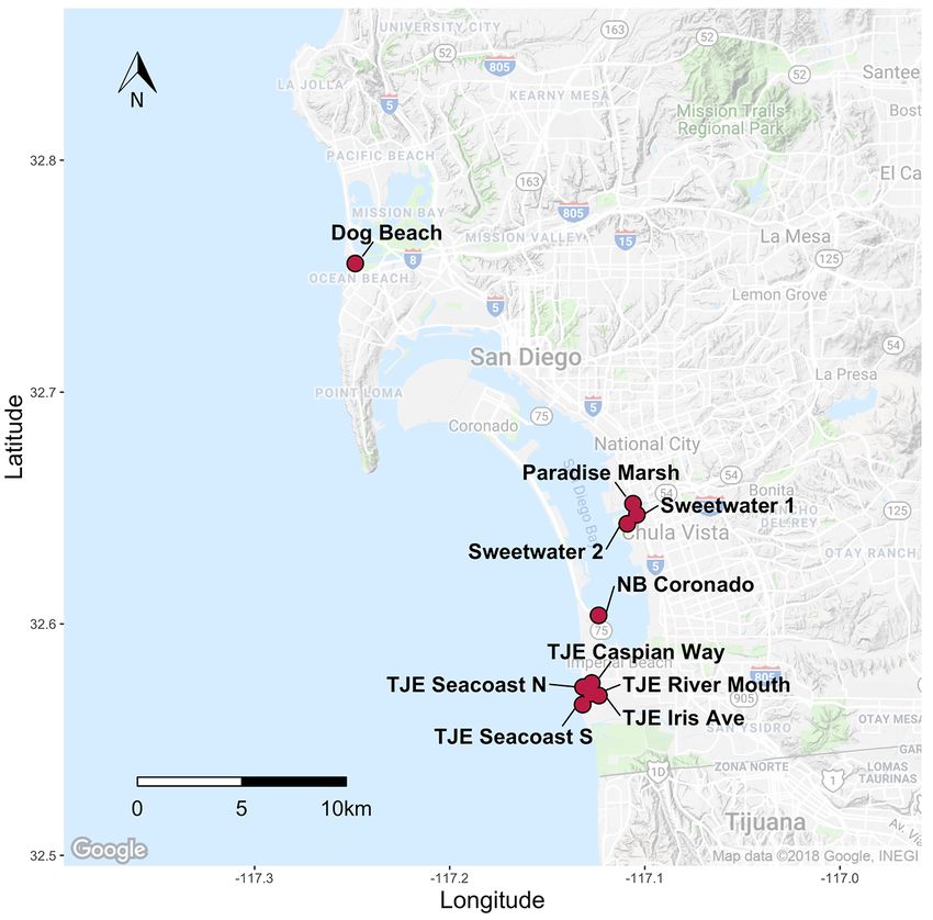
Contents
Acknowledgments ......................................................................................................................................... iii
Abstract ......................................................................................................................................................... 1
Introduction .................................................................................................................................................... 1
  Study Objectives ........................................................................................................................................ 3
Methods ......................................................................................................................................................... 3
     Sample Collection .................................................................................................................................. 3
     Flow Cytometry ...................................................................................................................................... 4
     Genomic Library Preparation ................................................................................................................. 4
     Genotyping and Analysis ....................................................................................................................... 4
     Management Ranking and Panel Discussion ........................................................................................ 5
       Genetic Differentiation Among Occurrences ...................................................................................... 6
       Genetic Diversity Within Occurrences ................................................................................................ 6
       Inbreeding and Relatedness Within Occurrences............................................................................... 6
       Occurrence Size and Field Data ......................................................................................................... 7
Results and Discussion ................................................................................................................................. 7
     Flow Cytometry ...................................................................................................................................... 7
  Species-Specific Genetic Structure Results and Discussion ...................................................................... 8
     Acanthomintha ilicifolia .......................................................................................................................... 8
     Baccharis vanessae ............................................................................................................................. 14
     Chloropyron maritimum ssp. maritimum .............................................................................................. 19
     Deinandra conjugens ........................................................................................................................... 27
     Dicranostegia orcuttiana ...................................................................................................................... 32
     Monardella viminea .............................................................................................................................. 37
  Management Rankings and Compatible Management Strategies............................................................ 42
References Cited ......................................................................................................................................... 43
Glossary ...................................................................................................................................................... 46
Appendix 1................................................................................................................................................... 48
Appendix 2................................................................................................................................................... 49

Figures
Figure 1. Map of sampled Acanthomintha ilicifolia occurrences.................................................................... 9
Figure 2. Genetic diversity statistics for Acanthomintha ilicifolia reported as mean values and standard
errors for each occurrence. Note the scale is unique to each dataset and should be considered before
comparing across plots. ............................................................................................................................... 10
Figure 3. Pairwise FST heatmap for Acanthomintha ilicifolia occurrences. Light color shading represents low
genetic differentiation, and dark color shading represents high genetic differentiation; values provided in
red. Note color scale is unique to each dataset and should not be compared across species. ................... 11
Figure 4. Principal component (PC) plot for Acanthomintha ilicifolia occurrences with PC1 on the horizontal
axis and PC2 on the vertical axis. Each point represents an individual sample, and each color and solid
ellipse represents an occurrence. Grey hashed ellipses identify occurrences in specific geographic regions.
Inset scree plot shows relative values of retained PCs, dimensional grid scale indicated in the upper right
corner of main plot. ...................................................................................................................................... 12

                                                                                      iv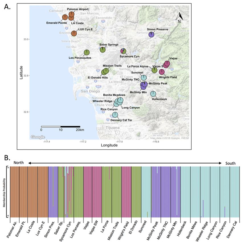
Figure 5. Maximum likelihood membership probability of Acanthomintha ilicifolia where color represents
probability of belonging to one of K = 5 genetic clusters. A, averaged by occurrence on map, and B,
ordered north to south, where each bar represents an individual. ............................................................... 13
Figure 6. Map of sampled Baccharis vanessae occurrences. ..................................................................... 15
Figure 7. Genetic diversity statistics for Baccharis vanessae reported as mean values and standard errors
for each occurrence. Note the scale is unique to each dataset and should be considered before comparing
across plots. ................................................................................................................................................ 16
Figure 8. Pairwise FST heatmap for Baccharis vanessae occurrences. Light color shading represents low
genetic differentiation, and dark color shading represents high genetic differentiation; values provided in
red. Note color scale is unique to each dataset and should not be compared across species. ................... 17
Figure 9. Principal component (PC) plot for Baccharis vanessae occurrences with PC1 on the horizontal
axis and PC2 on the vertical axis. Each point represents an individual sample, and each color and ellipse
represents an occurrence. Inset scree plot shows relative values of retained PCs, dimensional grid scale
indicated in the upper right corner of main plot. ........................................................................................... 18
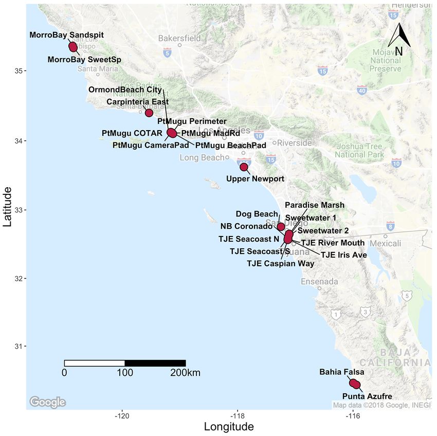
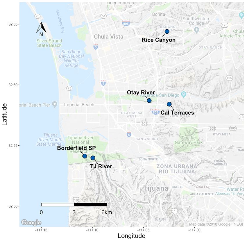
Figure 10. Map of sampled San Diego Chloropyron maritimum ssp. maritimum occurrences. ................... 20
Figure 11. Map of sampled regional Chloropyron maritimum ssp. maritimum occurrences. ....................... 21
Figure 12. Genetic diversity statistics for Chloropyron maritimum ssp. maritimum reported as mean values
and standard errors for each occurrence. Note the scale is unique to each dataset and should be
considered before comparing across plots. ................................................................................................. 22
Figure 13. Pairwise FST heatmap for Chloropyron maritimum ssp. maritimum occurrences. Light color
shading represents low genetic differentiation, and dark color shading represents high genetic
differentiation; values provided in red. Note color scale is unique to each dataset and should not be
compared across species. ........................................................................................................................... 23
Figure 14. Principal component (PC) plot for San Diego Chloropyron maritimum ssp. maritimum
occurrences with PC1 on the horizontal axis and PC2 on the vertical axis. Each point represents an
individual sample, and each color and ellipse represents an occurrence. Inset scree plot shows relative
values of retained PCs, dimensional grid scale indicated in the upper right corner of main plot. ................. 24
Figure 15. Principal component (PC) plot for regional Chloropyron maritimum ssp. maritimum occurrences
with PC1 on the horizontal axis and PC2 on the vertical axis. Each point represents an individual sample,
and each color and solid ellipse represents an occurrence. Grey hashed ellipse identifies San Diego
occurrences. Inset scree plot shows relative values of retained PCs, dimensional grid scale indicated in the
upper right corner of main plot. .................................................................................................................... 25
Figure 16. Maximum likelihood membership probability of regional Chloropyron maritimum ssp. maritimum
where color represents probability of belonging to one of K = 5 genetic clusters. A, averaged by occurrence
on map, and B, ordered north to south, where each bar represents an individual. ...................................... 26
Figure 17. Map of sampled Deinandra conjugens occurrences. ................................................................. 28
Figure 18. Genetic diversity statistics for Deinandra conjugens reported as mean values and standard
errors for each occurrence. Note the scale is unique to each dataset and should be considered before
comparing across plots. ............................................................................................................................... 29
Figure 19. Pairwise FST heatmap for Deinandra conjugens occurrences. Light color shading represents low
genetic differentiation, and dark color shading represents high genetic differentiation; values provided in
red. Note color scale is unique to each dataset and should not be compared across species. ................... 30
Figure 20. Principal component (PC) plot for Deinandra conjugens occurrences with PC1 on the horizontal
axis and PC2 on the vertical axis. Each point represents an individual sample, and each color and ellipse
represents an occurrence. Inset scree plot shows relative values of retained PCs, dimensional grid scale
indicated in the upper right corner of main plot. ........................................................................................... 31
Figure 21. Map of sampled Dicranostegia orcuttiana occurrences. ............................................................ 33
v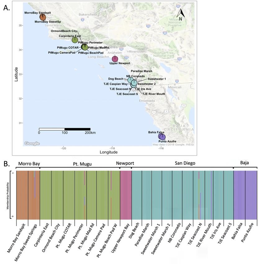
Figure 22. Genetic diversity statistics for Dicranostegia orcuttiana reported as mean values and standard
errors for each occurrence. Note the scale is unique to each dataset and should be considered before
comparing across plots. ............................................................................................................................... 34
Figure 23. Pairwise FST heatmap for Dicranostegia orcuttiana occurrences. Light color shading represents
low genetic differentiation, and dark color shading represents high genetic differentiation; values provided in
red. Note color scale is unique to each dataset and should not be compared across species. ................... 35
Figure 24. Principal component (PC) plot for Dicranostegia orcuttiana occurrences with PC1 on the
horizontal axis and PC2 on the vertical axis. Each point represents an individual sample, and each color
and ellipse represents an occurrence. Inset scree plot shows relative values of retained PCs, dimensional
grid scale indicated in the upper right corner of main plot............................................................................ 36
Figure 25. Map of sampled Monardella viminea occurrences. .................................................................... 38
Figure 26. Genetic diversity statistics for Monardella viminea reported as mean values and standard errors
for each occurrence. Note the scale is unique to each dataset and should be considered before comparing
across plots. ................................................................................................................................................ 39
Figure 27. Pairwise FST heatmap for Monardella viminea occurrences. Light color shading represents low
genetic differentiation, and dark color shading represents high genetic differentiation; values provided in
red. Note color scale is unique to each dataset and should not be compared across species. ................... 40
Figure 28. Principal component (PC) plot for Monardella viminea occurrences with PC1 on the horizontal
axis and PC2 on the vertical axis. Each point represents an individual sample, and each color and ellipse
represents an occurrence. Inset scree plot shows relative values of retained PCs, dimensional grid scale
indicated in the upper right corner of main plot. ........................................................................................... 41
Figure 1–1. Example histogram output from flow cytometry analysis; RN1 indicates peak position of
internal standard, and RN2 indicates peak position of sample. ................................................................... 48

Tables
Table 1. Mean and standard deviation of flow cytometry peak ratios by species. ......................................... 7
Table 2–1. Acanthomintha ilicifolia occurrence locations and summary statistics. ...................................... 49
Table 2–2. Baccharis vanessae occurrence locations and summary statistics. .......................................... 50
Table 2–3. Chloropyron maritimum ssp. Maritimum occurrence locations and summary statistics. ............ 51
Table 2–4. Deinandra conjugens occurrence locations and summary statistics.......................................... 52
Table 2–5. Dicranostegia orcuttiana occurrence locations and summary statistics. .................................... 53
Table 2–6. Monardella viminea occurrence locations and summary statistics. ........................................... 54
Table 2–7. Summary of management ranking decision, compatible potential management options, and
additional needed information by species. ................................................................................................... 55

                                                                                     vi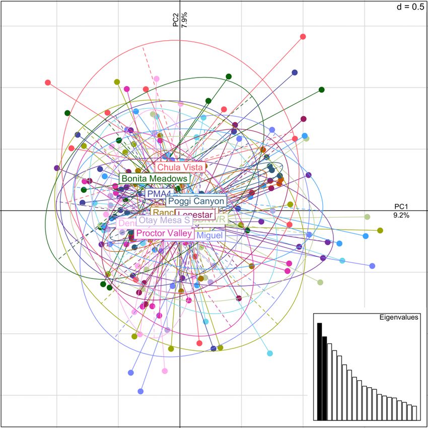
Conversion Factors
International System of Units to Inch/Pound
                       Multiply                               By                            To obtain
                                                          Mass
nanogram (ng)                                           3.527 × 10⁻¹¹ ounce, avoirdupois (oz)
picogram (pg)                                           3.527 × 10⁻¹⁴ ounce, avoirdupois (oz)

Datum
Vertical coordinate information is referenced to the North American Vertical Datum of 1988 (NAVD 88).
Horizontal coordinate information is referenced to the North American Datum of 1983 (NAD 83).

Abbreviations
AIC              Akaike information criterion
bp               base pair
BIC              Bayesian information criterion
CBI              Conservation Biology Institute
CPEN             Marine Corps Base Camp Pendleton
ddRAD            double-digest restriction-site associated DNA sequencing
DNA              deoxyribonucleic acid
IBD              isolation by distance
IMG              inspect and manage protocol
MCAS             Marine Corps Air Station
MSP              Management Strategic Plan
MPA              Management Plan Area
PCA              principal component analysis
PCR              polymerase chain reaction
qPCR             quantitative polymerase chain reaction
RSABG            Rancho Santa Ana Botanical Garden
SE               standard error
SNP              single nucleotide polymorphism
USDA             U.S. Department of Agriculture
USFWS            U.S. Fish and Wildlife Service
USGS             U.S. Geological Survey

                                                                   vii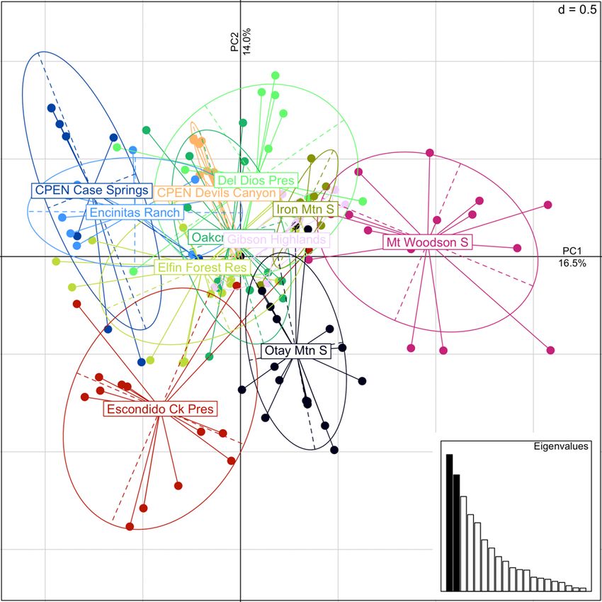
Population Genomic Surveys for Six Rare Plant
Species in San Diego County, California
By Elizabeth R. Milano and Amy G. Vandergast

Abstract
         San Diego County is a hotspot of biodiversity, situated at the intersection of the Baja
peninsula, the California floristic province, and the desert southwest. This hotspot is
characterized by a high number of rare and endemic species, which persist alongside a major
urban epicenter. San Diego County has implemented a strategic management plan that identifies
species, based on low numbers of occurrences or high level of threat, for which management
practices are recommended. In creating a management plan for rare species, it is important to
strike a balance between preserving locally adapted traits and maintaining genetic diversity, as
species’ ranges fluctuate in response to a changing climate and habitat fragmentation. This
project, in partnership with the San Diego Natural History Museum, aims to provide a reference
point for the current status of genetic diversity of rare plant species that will inform future
preservation and restoration efforts. We focused on six threatened or endangered plant species:
Acanthomintha ilicifolia, Baccharis vanessae, Chloropyron maritimum ssp. maritimum,
Deinandra conjugens, Dicranostegia orcuttiana, and Monardella viminea. For each species,
botanists from the San Diego Natural History Museum visited all known occurrences in San
Diego County and collected leaf tissue for genetic and cytological analysis. We then developed a
panel of genetic markers to estimate genetic diversity and population structure. This population
genetic survey provided insight into the amount of genetic differentiation across each species’
range, identified isolated occurrences potentially subject to inbreeding or genetic bottlenecks,
and identified areas that are rich sources of allelic diversity. Finally, we convened a panel of
experts to review results and compatible management options for each species. A summary of
the management workshop is included in this report. Overall, we found low genetic
differentiation among occurrences across the San Diego region for all species, with the exception
of A. ilicifolia. Relative inbreeding was low and consistent across sites, and genetic diversity
across sites was variable, with noted exceptions. These findings allow for a wide array of
management options that are compatible with panmictic population structure in five of the six
surveyed species.

Introduction
        The Management Strategic Plan (MSP) for western San Diego County has identified rare
plant species within the plan area for which management activities, such as enhancing population
sizes or establishing new occurrences, are ongoing or recommended based on low numbers of
individuals, low numbers of occurrences, or high risk of threat (table V3.App1A in San Diego
Management and Monitoring Program and The Nature Conservancy, 2017). However, the

                                                1
genetic diversity and genetic structure of these species are largely unknown, and the MSP
identifies conducting genetic surveys as a research need to inform development of
implementation plans, planned translocations, seed banking, and other management actions.
Genetic data provide information on plant population status, such as gene flow and
adaptive potential, which is useful when planning conservation management strategies
(Ellstrand and Elam, 1993; Frankham and others, 2002). Genetic factors, including ploidy and
levels of genetic relatedness among individuals, can influence compatibility and survivorship of
transplanted individuals or outcrossed offspring (McKay and others, 2005; Gibson and others,
2017). A key genetic concern when faced with restoration choices is determining the appropriate
balance between retaining local adaptation and maximizing overall diversity to avoid negative
inbreeding effects and retain the ability to respond to future environmental change (Weeks and
others, 2011; Harrisson and others, 2014). Understanding population genetic structure can aid in
this assessment by estimating the scale over which gene flow occurs and providing information
on the distribution of genetic diversity across individuals and occurrences (Hughes and others,
2008; Engelhardt and others, 2014). Here we use the term occurrence to refer to the primary unit
of management recognized by the MSP. Following the California Natural Diversity Database
definition of an element occurrence, two occurrences are unique if the distance between their
closest parts is ≥ 0.25 miles without regard to whether individuals interbreed (California Natural
Diversity Database, 2011). Population parameters that can be estimated with genetic data include
genetic differentiation among occurrences, genetic diversity within occurrences, and levels of
inbreeding and relatedness among individuals within occurrences (Ottewell and others, 2016).
Genetic differentiation among occurrences comprises the amount of total genetic
variation partitioned among occurrences and the genetic distinctiveness of occurrences or groups
of occurrences. Genetic differentiation among occurrences can arise over time when gene flow
(movement of pollen and seeds) is low among occurrences. This can be due to physical or
environmental barriers on the landscape or factors that reduce survivorship and interbreeding
among individuals with non-local genotypes (such as differences in ploidy or locally adaptive
traits). Gene flow can also be limited spatially, leading to a pattern of isolation by distance
(IBD), where genetic differentiation increases as distance between occurrences increases. When
gene flow is high among occurrences (and genetic differentiation is low), this may imply a
certain level of genetic redundancy across sites, in the sense of ecological redundancy of species
contributing to ecosystem resilience (Walker, 1992). Estimating levels of differentiation is useful
in selecting sets of compatible occurrences for seed or translocation sources.
Genetic variation provides the raw material for selection and diversification, and the
amount of genetic variation contained within a population is closely tied to population size,
connectivity, and thus persistence and adaptive potential (Frankham, 2005). Small occurrences—
those founded from just a few individuals or those that undergo frequent or extended genetic
bottlenecks— tend to have lower genetic diversity than those that are large or well-connected
via gene flow to other occurrences. Low genetic diversity can be correlated with increased
extinction risks and low adaptive potential (Spielman and others, 2004; Markert and others,
2010). If genetic diversity is very low, it may be useful to introduce new genetic material to the
occurrence to boost genetic diversity and to conduct management activities to support more
individuals in situ. When selecting occurrences for seed sources, higher diversity sites might be
preferable to lower diversity sites, if genetic similarity among sites is also high. Loss of genetic
diversity within sites will also increase the level of divergence between them because of the
2random loss of alleles (genetic drift). Signatures of high genetic divergence and low genetic
diversity often occur together (Allendorf, 1986; Slatkin, 1987; Young and others, 1996).
In predominantly outcrossing species, as populations become small it is more likely for
close relatives to interbreed or for selfing to occur (Wright, 1938, 1978). Such small populations
will have higher levels of inbreeding and relatedness than larger ones with random mating.
Breeding between relatives lowers heterozygosity and can reduce the fitness of offspring
(inbreeding depression), which can then adversely affect population growth rates (Crnokrak
and Roff, 1999; Williams, 2001). Although levels of inbreeding and relatedness can be estimated
using genetic information, determining the level of inbreeding depression also requires gathering
data on individual fitness (Crnokrak and Roff, 1999).
Study Objectives
We examined the genetic population structure of six priority plant species throughout the
San Diego Management Plan Area (MPA): Acanthomintha ilicifolia, Baccharis vanessae,
Chloropyron maritimum ssp. maritimum, Deinandra conjugens, Dicranostegia orcuttiana, and
Monardella viminea. With the exception of D. orcuttiana, all of these species are federally listed
as endangered or threatened. To understand the genetic structure of each of these species, we
obtained samples from most known occurrences of the six priority species, developed and
analyzed a panel of genetic markers to assess population diversity and divergence, and
performed a comparative cytological analysis. Results were then summarized according to a
conservation prioritization and decision-making framework (Ottewell and others, 2016) to
inform land managers.
Following genetic and cytological analysis, we convened a panel of ecologists and rare
plant experts to review results and identify compatible management options for each species
relative to their respective MSP objectives. This report includes those options on genetic
management of occurrences, addresses MSP objectives involving seed banking and seed bulking
needs for each species, and identifies information gaps that, if addressed, could further support
management efforts. In addition to supporting regional conservation efforts for the San Diego
MPA, these results provide scientific information for the U.S. Fish and Wildlife Service
(USFWS) for the five Federally listed species. Finally, these data provide a snapshot for
monitoring genetic diversity trends over time in response to future disturbances or restoration
actions.
Methods
Sample Collection
Samples were collected in the spring and fall of 2016 and the spring of 2017 by the San
Diego Natural History Museum (2018). San Diego Natural History Museum botanists attempted
to visit and sample from all known occurrences of each priority species within the San Diego
MPA. In some cases, additional occurrences were sampled on lands not managed as part of the
MSP. These samples were included for analysis context only. Any compatible management
options are provided for MSP occurrences.
Collections were made from 20 randomly selected plants from each occurrence, though
some occurrences contained fewer than 20 individuals and so fewer were sampled (San Diego
Natural History Museum, 2018). Sampled plants were distributed evenly throughout the spatial
3extent of each occurrence. Five plants from each occurrence were further sampled for flow
cytometry analysis. Leaf tissue for DNA (deoxyribonucleic acid) extraction was collected into
coin envelopes and assigned a unique identifier. Envelopes were stored with color-indicating
silica gel desiccant in plastic bins at room temperature. Containers were gently shaken daily to
expedite moisture extraction from the leaf tissue. Silica gel beads were changed regularly when
fully saturated.
Flow Cytometry
Fresh leaf tissue was shipped overnight to the U.S. Department of Agriculture (USDA)
Forest Service Shrub Science Laboratory in Provo, Utah, for flow cytometric analysis. All
samples were run on a Cyflow Space cytometer (Sysmex Corporation) with Atriplex canescens
(1C-value = 1.64 pg) 2× or 4× as an internal standard. The value of each sample was determined
by a ratio of the sample peak position to the internal standard peak position, where peak position
is indicated by the mean-x value of the designated peaks on the histogram output from the flow
cytometer (fig. 1–1). The peak ratio (sample/standard) mean and standard deviation were
calculated for each species. Multiple levels of ploidy within species would be suspected if
twofold differences in peak ratios were detected.
Genomic Library Preparation
Genomic DNA was extracted from 15 samples per occurrence. Additional collected
samples were used as reserve in case of tissue damage or low yield of DNA following extraction.
In total, 1,273 samples were prepared for genetic analysis across all 6 species and
77 occurrences. Extractions were performed using either the Qiagen DNeasy Plant Mini Kit
(Qiagen, Valencia, California) or the E-Z 96® Plant DNA Kit (Omega Bio-tek Inc., Norcross,
Georgia) according to respective manufacturers guidelines, with the addition of a 1-hour room
temperature incubation during the first elution. Reduced representation genomic libraries were
prepared using a modified double-digest restriction-site associated DNA sequencing (ddRAD)
scheme (Peterson and others, 2012). In brief, 300 nanograms (ng) of DNA were cut with EcoRI
and SbfI restriction enzymes. In-line barcodes were ligated onto the SbfI cut site, fragments
were size-selected on a Pippin Prep (Sage Science, Inc., Beverly, Massachusetts) at a 350 ± 50
base pairs (bp) range, and Illumina sequencing adaptors were ligated onto the EcoRI cut site.
Each library, containing 16 multiplexed samples, was polymerase chain reaction (PCR)
amplified for 14 cycles with the addition of a unique library index sequence and quantified with
quantitative PCR (qPCR). This dual index scheme allowed for multiple libraries to be sequenced
in a single sequencing lane. In total, 101 libraries were pooled (8–12 libraries per lane, U.S.
Geological Survey [USGS] data release https://doi.org/10.5066/P9OWNCG8) into 11–100 bp
paired-end HiSeq 4000 lanes (Illumina, Inc., San Diego, California). Libraries were quantified,
pooled, and sequenced at the Vincent J. Coates Genomic Sequencing Laboratory at University of
California, Berkeley (Berkeley, California).
Genotyping and Analysis
Raw sequence demultiplexing, quality filtering, and genotyping was performed using the
software Stacks v2.0b8 (Catchen and others, 2011) on the USGS Yeti High Performance
Computing Cluster. Clustering, assembly, and filtering parameters were optimized for each
species using a subset of high coverage individuals, comprised of 25–35 percent of all samples,
4evenly distributed across collection locations, following the r80 method by Paris and others
(2017). This sample subset was also used to create the locus catalog (cstacks) for the full Stacks
genotyping pipeline. We report the following Stacks parameters for each species: M, maximum
number of mismatches between stacks within individuals; n, maximum number of mismatches
between stacks between individuals; r, minimum percentage of individuals in an occurrence
required to process a locus for that occurrence; and p, minimum number of occurrences a locus
must be present in to process a locus (Catchen and others, 2011). Genetic diversity statistics,
including pairwise genetic differentiation (FST) expected heterozygosity (He), number of private
alleles, and inbreeding (FIS), were calculated using the populations program in Stacks, while
filtering for a single bi-allelic single nucleotide polymorphism (SNP) per locus (detailed in
Hohenlohe and others, 2010). Specifically, populations used an analysis of molecular variance
framework to calculate a nucleotide-level FST value, a measure of genetic variation within and
between sites, between each pair of occurrences (Weir, 1996; Rochette and Catchen, 2017). He, a
measure of genetic diversity within site, was calculated as the mean expected frequency of
heterozygotes under Hardy-Weinberg conditions (Catchen and others, 2013), and private alleles
were considered so if only found in one occurrence. FIS, a measure of genetic variation within an
individual, was calculated as the degree of difference between observed and expected
heterozygotes within occurrences (Wright, 1931, 1978; Catchen and others, 2013). Relatedness
(r) within each occurrence was calculated using the Queller and Goodnight (1989) estimator, as
implemented in the package related v1.0 (Pew and others, 2015) in R v3.3.2 (R Core Team,
2016), to provide further insight into within-site dynamics. To account for missing data,
occurrence sample size is presented as an average of the number of individuals with an allele call
at each locus.
Genetic clustering analyses were used to explore the pattern of genetic structure in each
species. We used two methods, a principal component analysis (PCA) and maximum-likelihood
K-means clustering (snapclust; Beugin and others, 2018), to identify differences in allele
frequencies across each set of genetic markers. For snapclust, an optimal number of clusters (K)
was chosen using both the Bayesian information criterion (BIC) and the Akaike information
criterion (AIC), as implemented in snapclust.choose.k. Finally, a mantel test was used to test for
a significant pattern of isolation by distance (IBD). Genetic clustering and spatial analyses were
implemented in the R package adegenet v2.1.1 (Jombart, 2008). Raw sequence data are available
at http://www.ncbi.nlm.nih.gov/bioproject/484956, and final genetic marker datasets for each
species are provided as a USGS data release at https://doi.org/10.5066/P9OWNCG8.
Management Ranking and Panel Discussion
We convened a group of experts to review genetic data results for six rare plant species
throughout San Diego County to determine population status and discuss compatible
management options and outstanding information needs for occurrences on conservation lands
contained within the San Diego MPA. We used a rubric to rank species on a scale of
management intensity based on three types of genetic information.
We generally followed the strategies of Ottewell and others (2016) to assign species into
management categories using three levels of genetic information with relevance for
conservation: genetic differentiation (FST) among occurrences, genetic diversity (measured as
expected heterozygosity, He) and private alleles within occurrences, and inbreeding (FIS) and
relatedness (r) among individuals within occurrences (figure 1 in Ottewell and others, 2016).
Genetic clustering and IBD results also contributed to determining genetic differentiation among
5occurrences. Additionally, we considered other occurrence characteristics from field data
gathered at the time of genetic sample collection or during implementation of the inspect and
manage protocol (IMG) for plant occurrence monitoring in the MPA ( San Diego Management
and Monitoring Program, 2018a).
Genetic Differentiation Among Occurrences
First, we ranked genetic differentiation among occurrences as high or low. We used three
types of metrics to assess genetic differentiation: pairwise FST, IBD, and genetic clustering (see
section “Genotyping and Analysis”). Genetic differentiation was considered high if most
estimates of FST between occurrence pairs were significantly different from zero and (or) if
multiple genetic clusters were detected. Isolation by distance was supported if a significantly
positive relationship was determined between pairwise genetic distance and the geographic
distances between occurrences. Genetic differentiation was considered low if most estimates of
FST between occurrence pairs were low and if PCA and clustering methods indicated a single
genetic cluster best represented structure across the study area.
Genetic Diversity Within Occurrences
We ranked genetic diversity within occurrences as low or high based on average expected
heterozygosity (He) and number of private alleles (see section “Genotyping and Analysis”). We
assigned a rank of high if all assessed occurrences had relatively even average genetic diversity.
We assigned a rank of low if one or more occurrences had lower average genetic diversity
compared to other sites. We mainly relied on among occurrence comparisons within species
because in most cases (with the exception of C. maritimum spp. maritimum) we did not have
samples from outside of the San Diego MPA to compare. We also attempted to relate any
unusually low diversity aggregations with known historical factors such as notably low census
size or whether the occurrence was outplanted or natural. Although we could also consider
whether average genetic diversity within a particular species was generally high or low in
comparison to other species examined in this study, there are several important caveats to
comparing across species. Notably, each species was surveyed at a different set of unique loci
across the genome. In addition, the species surveyed are not closely related, and so each is
subject to a unique evolutionary history, life history traits, and breeding structure that will
generally affect genomic diversity (Hamrick and Godt, 1996).
Inbreeding and Relatedness Within Occurrences
Finally, we examined statistics to determine individual levels of inbreeding or genetic
relatedness within occurrences as low or high. We examined coefficients of inbreeding (FIS) and
relatedness (r) among individuals within occurrences. If inbreeding and relatedness coefficients
had error bars that included zero, we assumed that inbreeding and relatedness were non-
significant and met expectations under random mating conditions. We categorized the inbreeding
as high if multiple occurrences had inbreeding with values greater than zero. Negative estimates
are also possible and can be interpreted as individuals being less related than expected in a
randomly mating population. It should be noted that the accuracy of inbreeding and relatedness
estimators can be affected by small numbers of markers, small sample sizes within populations,
and genotyping errors (Pemberton, 2004; Wang, 2007, 2017). As with genetic diversity,
inbreeding and genetic relatedness should be measured against a reference population and should
not be compared across species because these measures are highly dependent on the mating
6system, particularly the level of self-compatibility and frequency of self-fertilization. Here, we
compared occurrences within species to each other to determine whether any outliers, that may
indicate unusual levels of mating between close relatives, were present.
Occurrence Size and Field Data
We compiled existing data for each occurrence of each species for review. These data
included estimates of abundance, aspect, soil texture, vegetation community, descriptions of
morphological differences among plants within occurrences, and noted disturbance within
occurrences (San Diego Natural History Museum, 2018). If available, we also compiled IMG
survey abundance and disturbance estimates (San Diego Management and Monitoring Program,
2018a). Disturbances included presence of non-native species, physical disturbance or habitat
modifications (trails, trampling, illegal dumping restoration activities), altered hydrology, and
recent fire.
Rankings were then discussed using compatible management options (table 1; Ottewell
and others, 2016) as a starting guide. Discussion of results for each species centered around two
major themes: (1) compatible management actions or strategies that could be applied and (2)
existing data or information gaps for each species. Species-specific threats and natural history
were taken into account when developing compatible management options.
Results and Discussion
In general, with the genetic loci we analyzed, we found low genetic differentiation for all
species across the San Diego region, with the exception of A. ilicifolia. Relative genetic diversity
between occurrences was variable, and average inbreeding values were relatively low and
consistent across sites. These findings of panmictic population structure in most species are
compatible with a wide array of management options.
Flow Cytometry
We did not find evidence of multiple levels of ploidy within species. The greatest
variation in peak ratios was within C. maritimum spp. maritimum (mean = 4.18; standard
deviation = 0.77), but we did not observe a twofold difference between any samples that would
indicate doubled (or greater) genome size variation.
Table 1. Mean and standard deviation of flow cytometry peak ratios by species.
SPECIES RATIO RATIO
MEAN ST. DEV.
A. ilicifolia 7.24 0.37
B. vanessae 4.09 0.28
C. maritimum spp. 5.19 0.77
maritimum
D. conjugens 4.18 0.44
D. orcuttiana 3.64 0.29
M. viminea 6.67 0.32
7Species-Specific Genetic Structure Results and Discussion
Acanthomintha ilicifolia
Acanthomintha ilicifolia (Lamiaceae) is an annual herb restricted to clay lenses in San
Diego County and northwest Baja California, Mexico. Occurrence size estimates can fluctuate
annually, sometimes by an order of magnitude (U.S. Fish and Wildlife Service, 2009a) and are
widely variable across the region. Notably, 750,000 individuals were found in Sycamore Canyon
in 2017; only 17,500 were found in 2016. Similarly, 15 plants were counted on the southwest
slope of McGinty Mountain in 2016, followed by 100 plants in 2017 (San Diego Management
and Monitoring Program, 2018a; San Diego Natural History Museum, 2018).
We analyzed 350 individuals from 24 occurrences (fig. 1; table 2–1). Raw 100-bp paired-
end sequence reads totaled 806,037,612 with an average of 2,202,288.56 (standard deviation =
926,614.29) paired-end reads per individual. The final genetic marker dataset consisted of
195 independent SNP loci, using the following stacks parameters: M = 3, n = 3, r = 0.8, p = 18.
Inbreeding was low and consistent across sites, whereas relatedness ranged from 0.16 (± 0.02
SE; standard error) to 0.95 (± 0.01 SE). Genetic diversity (He) ranged from 0.007 (± 0.002 SE) at
Emerald Pointe to 0.074 (± 0.01 SE) at Bonita Meadows (fig. 2; table 2–1). Genetic
differentiation (FST) between sites ranged from 0.036 to 0.5, where pairwise comparisons with
Emerald Pointe were among the highest values (fig. 3). Results from genetic clustering analyses
showed distinct groupings of occurrences that correspond to geographic regions. A PCA
revealed three clusters that correspond to a northern group of occurrences (Palomar Airport,
Emerald Pointe, La Costa, and Lux Canyon), an eastern group (Wright’s Field, Viejas, Viejas
Southwest, and part of La Force Alpine), and a central group that contained the remainder of
occurrences (fig. 4). Maximum-likelihood clustering showed five genetic clusters that not only
distinguish the northern and eastern groups, but break up the central occurrences into one
distinctly southern group and two central groups (fig. 5). The largest occurrence, Sycamore
Canyon, contained individuals assigned to all except the northern cluster. A mantel test for IBD
revealed a significant correlation between genetic and geographic distance matrices (R2 = 0.623;
p < 0.001; 999 permutations) that is consistent with genetic clustering among geographic
regions.
Given low genetic diversity within Emerald Pointe and a small occurrence size estimate
(39 plants in 2016; San Diego Natural History Museum, 2018), large among-site differences
could reflect genetic drift owing to loss of genetic diversity within this site as well as loss of
connectivity with all but the closest neighboring occurrences. Conservation Biology Institute
(Conservation Biology Institute, 2018) has binned all known occurrences into “regional
population structure” (not to be confused with population genetic structure) categories based on
population size, proximity to other occurrences, and management opportunity, among other
factors. We found similarities between CBI’s categories and genetic clustering in the northern
and eastern groupings of occurrences as identified in the PCA, but we also found that the central
occurrences are genetically more connected than expected when categorizing based on habitat
and size. We found no evidence of multiple levels of ploidy across sampled occurrences (see
section “Flow Cytometry”). This is in contrast to a recent study by DeWoody and others (2018)
that found cytogenetic variation, in low proportions, within two occurrences adjacent to, but not
overlapping with, occurrences we sampled in the northern and eastern regions. DeWoody and
other’s (2018) eastern occurrence now no longer exists, and we did not have access to the
northern occurrence in question. Although our cytology results differ, both studies did find
8evidence of distinct population genetic structure across the region, which is an important
consideration when developing an assisted migration plan.
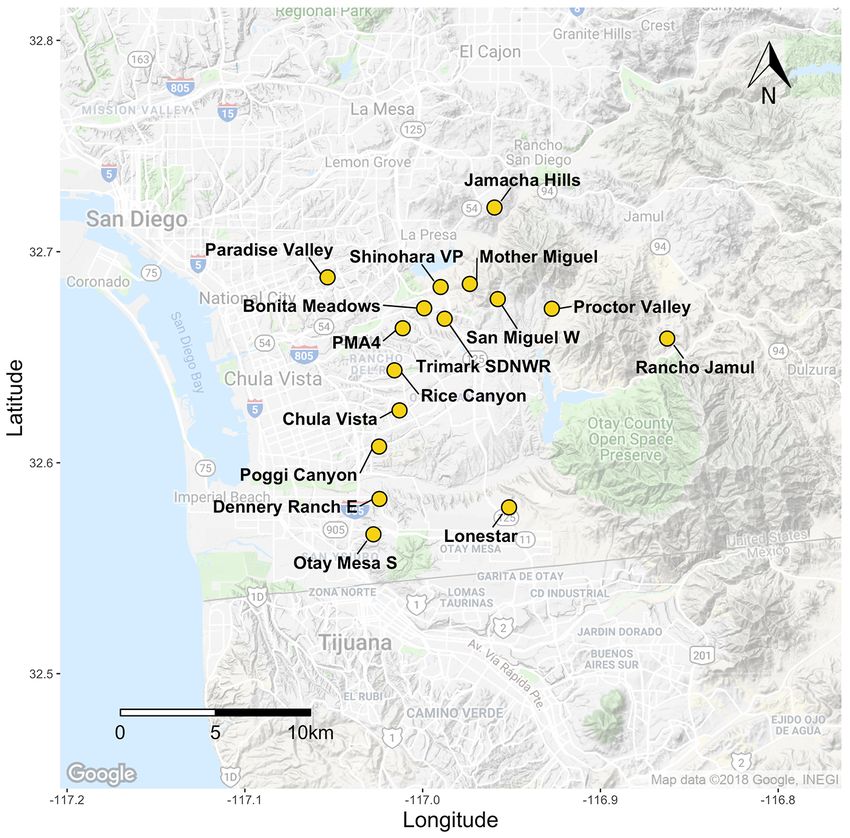
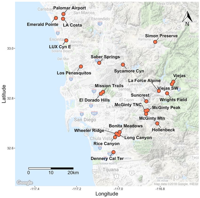
Figure 1. San Diego County map of sampled Acanthomintha ilicifolia occurrences. Cyn, Canyon; E, East;
Mtn, Mountain; SW, Southwest; Ter, Terraces; TNC, The Nature Conservancy.
9Figure 2. Genetic diversity statistics for Acanthomintha ilicifolia reported as mean values and standard
errors for each occurrence. Note the scale is unique to each dataset and should be considered before
comparing across plots. Cyn, Canyon; E, East; Mtn, Mountain; SW, Southwest; Ter, Terraces; TNC, The
Nature Conservancy.
10Figure 3. Pairwise FST (genetic differentiation) heatmap for Acanthomintha ilicifolia occurrences. Light color
shading represents low genetic differentiation, and dark color shading represents high genetic
differentiation; values provided in red. Note color scale is unique to each dataset and should not be
compared across species. Cyn, Canyon; E, East; Mtn, Mountain; SW, Southwest; Ter, Terraces; TNC, The
Nature Conservancy.
11Northern occurrences
Eastern occurrences
Figure 4. Principal component (PC) plot for Acanthomintha ilicifolia occurrences with PC1 on the horizontal
axis and PC2 on the vertical axis. Each point represents an individual sample, and each color and solid
ellipse represents an occurrence. Grey hashed ellipses identify occurrences in specific geographic regions.
Inset scree plot shows relative values of retained PCs, dimensional grid scale indicated in the upper right
corner of main plot. Cyn, Canyon; E, East; Mtn, Mountain; SW, Southwest; Ter, Terraces; TNC, The Nature
Conservancy.
12Figure 5. Maximum likelihood membership probability of Acanthomintha ilicifolia where color represents
probability of belonging to one of K = 5 genetic clusters. A, averaged by occurrence on map, and B,
ordered north to south, where each bar represents an individual. Cyn, Canyon; E, East; Mtn, Mountain;
SW, Southwest; Ter, Terraces; TNC, The Nature Conservancy.
13Baccharis vanessae
Baccharis vanessae (Asteraceae) is an herbaceous dioecious shrub endemic to San Diego
County. It occurs in dense chaparral vegetation (Beauchamp, 1980) in a patchy distribution from
Marine Corps Base Camp Pendleton (CPEN) in the north to Otay Mountain in the south.
Outplanting was attempted at a single site in San Dieguito County Park, but success has not been
reported and the occurrence is presumed extirpated (Beauchamp, 1980; U.S. Fish and Wildlife
Service, 2011). Recruitment is low at extant sites, and no seedlings have been observed since
1991. This may be due to dependence on regular fire cycles and (or) maintaining viable male and
female plants in close proximity (U.S. Fish and Wildlife Service, 2011).
We analyzed 133 individuals from 11 occurrences, 2 of which were newly discovered
during this study and located on CPEN (fig. 6; table 2–2). Raw 100-bp paired-end sequence
reads totaled 377,644,136 with an average of 2,586,603.67 (standard deviation = 2,711,797.03)
paired-end reads per individual. The final genetic marker dataset consisted of 45 independent
SNP loci using the following Stacks parameters: M = 4, n = 4, r = 0.7, p = 7. Inbreeding was
effectively zero for all sites, whereas relatedness ranged from –0.05 (± 0.05 SE) to 0.6 (± 0.03
SE) with the majority of sites falling between 0.4 and 0.6. Genetic diversity (He) was generally
low but consistent, ranging from 0.04 (± 0.02 SE) at CPEN Devil’s Canyon to 0.09 (± 0.03 SE)
at Oakcrest Park (fig. 7; table 2–2). Differentiation (FST) between sites ranged from 0.032 to
0.235 (fig. 8), and though we did not find any distinct genetic clusters (fig. 9) or evidence of
isolation by distance, Mount Woodson, Otay Mountain, and Escondido Creek were slightly more
differentiated than the main cluster of occurrences.
Baccharis vanessae was only first described in 1980 in and around Encinitas, California
(Beauchamp, 1980), but we did not find evidence that occurrences found outside of this locale
(that is Otay Mountain and CPEN) were genetically distinct from the central occurrences. This
connectivity through gene flow could indicate that there are additional unknown populations or
that long distance dispersal can occur. Additional undocumented populations would not be
surprising given that B. vanessae is somewhat cryptic on the landscape and can be difficult to
identify in its preferred dense chaparral environment. Male and female plants can only be
differentiated by floral morphology; unfortunately, not all plants were flowering during
collection, so we could not compare sex ratios between occurrences. It is concerning that verified
recruitment has not been recorded during field visits. Other species of Baccharis are known to
have a short seed viability timeframe (U.S. Fish and Wildlife Service, 2011), so we do not expect
multiple generations of seeds to be stored in the seedbank.
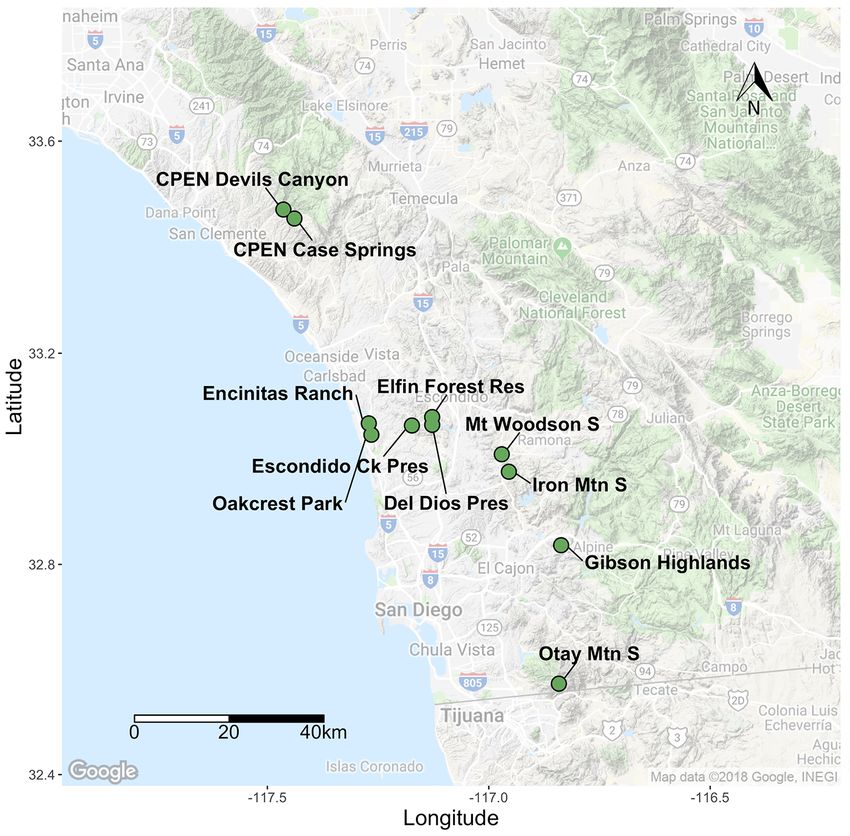
14Figure 6. San Diego County map of sampled Baccharis vanessae occurrences. Ck, Creek; CPEN, Marine
Corps Base Camp Pendleton; Mt, Mount; Mtn, Mountain; Pres, Preserve; Res, Reserve; S, South.
15Figure 7. Genetic diversity statistics for Baccharis vanessae reported as mean values and standard errors
for each occurrence. Note the scale is unique to each dataset and should be considered before comparing
across plots. Ck, Creek; CPEN, Marine Corps Base Camp Pendleton; Mt, Mount; Mtn, Mountain; Pres,
Preserve; Res, Reserve; S, South.
16Figure 8. Pairwise FST (genetic differentiation) heatmap for Baccharis vanessae occurrences. Light color
shading represents low genetic differentiation, and dark color shading represents high genetic
differentiation; values provided in red. Note color scale is unique to each dataset and should not be
compared across species. Ck, Creek; CPEN, Marine Corps Base Camp Pendleton; Mt, Mount; Mtn,
Mountain; Pres, Preserve; Res, Reserve; S, South.
17Figure 9. Principal component (PC) plot for Baccharis vanessae occurrences with PC1 on the horizontal
axis and PC2 on the vertical axis. Each point represents an individual sample, and each color and ellipse
represents an occurrence. Inset scree plot shows relative values of retained PCs, dimensional grid scale
indicated in the upper right corner of main plot. Ck, Creek; CPEN, Marine Corps Base Camp Pendleton; Mt,
Mount; Mtn, Mountain; Pres, Preserve; Res, Reserve; S, South.
18Chloropyron maritimum ssp. maritimum
Chloropyron maritimum ssp. maritimum (Orobanchaceae) is a hemiparasitic annual
halophyte found in salt marshes from Morro Bay, California, to Punta Azufre in northern Baja
California, Mexico. It is self-compatible and pollinated by a number of bee species. Host plant
species are unconfirmed and appear to be variable, depending on location (U.S. Fish and
Wildlife Service, 2009b). Two reintroduction projects have been attempted in the species,
including one at Sweetwater Marsh in San Diego County that was planted with seeds from
multiple occurrences around the Tijuana Estuary.
For this species in particular, we obtained samples from all known occurrences in San
Diego as well as additional occurrences spanning the range of C. maritimum ssp. maritimum
from Punta Azufre in Baja California, Mexico, to Morro Bay, California. In total, we analyzed
311 individuals from 22 occurrences across the range; 10 of those occurrences were in San
Diego County (figs. 10, 11; table 2–3). Raw 100-bp paired-end sequence reads totaled
592,586,084 with an average of 1,905,421.49 (standard deviation = 1,424,316.67) paired-end
reads per individual. The final genetic marker dataset consisted of 111 independent SNP loci,
using the following stacks parameters: M = 4, n = 4, r = 0.7, p = 15. For the sites located in San
Diego County, inbreeding was effectively zero, whereas relatedness ranged from –0.13 (± 0.07
SE) to 0.76 (± 0.05 SE). Genetic diversity (He) ranged from 0.015 (± 0.01 SE) at Paradise Marsh
to 0.085 (± 0.04 SE) at Tijuana Estuary River Mouth (fig. 12; table 2–3). The average He for San
Diego occurrences was 0.052, in contrast to the rangewide average He of 0.041, and the range
wide average He excluding San Diego occurrences of 0.032, indicating that San Diego is a
relatively diverse area for this species. Differentiation (FST) between sites ranged from 0.001 to
0.32 in San Diego (fig. 13), and we did not find any distinct genetic clusters or evidence of IBD
(fig. 14). However, we did find distinct genetic clusters rangewide that correspond to distinct
geographic locations. A PCA showed three clusters that correspond to San Diego, Naval Air
Station Point Mugu, and all other sites (fig. 15), and maximum-likelihood clustering revealed
five distinct clusters that correspond to regional sampling locations (fig. 16).
We found very little evidence of population structure within San Diego County but did
observe that genetic diversity is highest for the Tijuana Estuary occurrences, compared to the
Sweetwater Marsh transplanting locations and other San Diego marshes. A reintroduction project
in Seal Beach, California, closest to the Newport occurrence, was unsuccessful after several
attempts (U.S. Fish and Wildlife Service, 2009b), whereas the Sweetwater Marsh reintroduced
occurrences still support healthy plants. However, it is especially important to maintain large
numbers of individuals at transplanted sites to counteract the effects of genetic drift. Regionwide,
we do see evidence of genetic structure tightly correlated with geographic location. Although it
is noted that common co-occurring species are found to be influenced by tidal movement, and C.
maritimum ssp. maritimum seeds can float for up to 50 days (Hopkins and Parker, 1984; U.S.
Fish and Wildlife Service, 2009b), many historical occurrences in Los Angeles County, San
Bernardino County, and Orange County, including three inland sites, are now extirpated. This
has most likely reduced the connectivity of the San Diego occurrences to the more northern
locations, though no dispersal studies have been conducted.
19You can also read