Wind turbine load validation in wakes using wind field reconstruction techniques and nacelle lidar wind retrievals - WES
←
→
Page content transcription
If your browser does not render page correctly, please read the page content below
Wind Energ. Sci., 6, 841–866, 2021
https://doi.org/10.5194/wes-6-841-2021
© Author(s) 2021. This work is distributed under
the Creative Commons Attribution 4.0 License.

          Wind turbine load validation in wakes using wind field
                 reconstruction techniques and nacelle
                           lidar wind retrievals
                          Davide Conti1 , Vasilis Pettas2 , Nikolay Dimitrov1 , and Alfredo Peña1
                   1 Department of Wind Energy, Technical University of Denmark, Frederiksborgvej 399,
                                                 4000 Roskilde, Denmark
             2 Stuttgart Wind Energy (SWE), University of Stuttgart, Allmandring 5b, 70569 Stuttgart, Germany

                                      Correspondence: Davide Conti (davcon@dtu.dk)

                               Received: 3 September 2020 – Discussion started: 24 September 2020
                             Revised: 1 March 2021 – Accepted: 15 April 2021 – Published: 7 June 2021

       Abstract. This study proposes two methodologies for improving the accuracy of wind turbine load assessment
       under wake conditions by combining nacelle-mounted lidar measurements with wake wind field reconstruction
       techniques. The first approach consists of incorporating wind measurements of the wake flow field, obtained from
       nacelle lidars, into random, homogeneous Gaussian turbulence fields generated using the Mann spectral tensor
       model. The second approach imposes wake deficit time series, which are derived by fitting a bivariate Gaussian
       shape function to lidar observations of the wake field, on the Mann turbulence fields. The two approaches are nu-
       merically evaluated using a virtual lidar simulator, which scans the wake flow fields generated with the dynamic
       wake meandering (DWM) model, i.e., the target fields. The lidar-reconstructed wake fields are then input into
       aeroelastic simulations of the DTU 10 MW wind turbine for carrying out the load validation analysis. The power
       and load time series, predicted with lidar-reconstructed fields, exhibit a high correlation with the corresponding
       target simulations, thus reducing the statistical uncertainty (realization-to-realization) inherent to engineering
       wake models such as the DWM model. We quantify a reduction in power and loads’ statistical uncertainty by
       a factor of between 1.2 and 5, depending on the wind turbine component, when using lidar-reconstructed fields
       compared to the DWM model results. Finally, we show that the number of lidar-scanned points in the inflow and
       the size of the lidar probe volume are critical aspects for the accuracy of the reconstructed wake fields, power,
       and load predictions.

1   Introduction                                                   turbine responses and inducing high fatigue damage (Larsen
                                                                   et al., 2013). Moreover, small turbulence eddies that result
Wind turbines operating under wake conditions experience           from the breakdown of the tip vortices can cause small fa-
higher loading and lower power productions than those op-          tigue load cycles (Madsen et al., 2005). Thus, aeroelastic
erating under wake-free conditions (Barthelmie et al., 2009;       analysis of wind turbines operating under wake conditions
Larsen et al., 2013). The wake-induced velocity deficit and        requires detailed modeling of the wake flow fields.
its meandering are critical aspects in both loads and power           To date, detailed predictions of wake-generated turbulence
analyses (Madsen et al., 2010; Doubrawa et al., 2017). The         can be achieved with large eddy simulation (LES); however,
former reduces the inflow wind speed and causes unbalanced         the computational cost is prohibitive when large numbers of
aerodynamic load distribution at the rotor, which in turn in-      simulations are required. This makes engineering wake mod-
duces high load cycle amplitudes in the whole wind turbine         els a practical alternative for certain applications. For de-
structure (Lee et al., 2012). The latter is the main source of     sign load evaluation, the IEC 61400-1 standard (IEC, 2019)
wake-added turbulence (Madsen et al., 2010), affecting wind

Published by Copernicus Publications on behalf of the European Academy of Wind Energy e.V.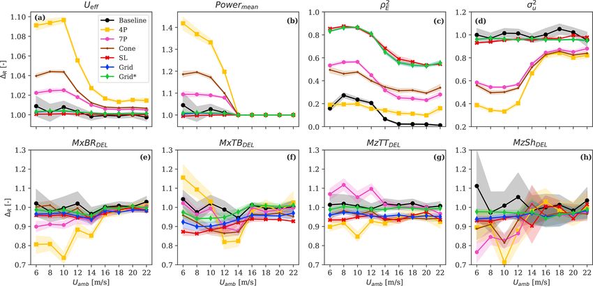
842                        D. Conti et al.: Wind turbine load validation in wakes using wind field reconstruction techniques

recommends the dynamic wake meandering (DWM) model,               power and loads in a validation analysis, it is essential to ac-
among other low-order engineering wake models.                    curately reconstruct wake meandering time series.
   The DWM model considers wakes to act as passive tracers           Alternative load verification procedures are being explored
displaced in the lateral and vertical directions by the large     to potentially reduce the statistical and modeling uncertainty
eddies of the atmospheric flow (Madsen et al., 2010). The         in engineering wake models and replace measurements from
wake field is modeled as a “cascade” of quasi-steady velocity     masts with those from Doppler lidars (Dimitrov et al., 2019;
deficits emitted by the source turbine that meander through       Reinwardt et al., 2020; Conti et al., 2020). Lidars can pro-
a pre-calculated stochastic meandering path and that are ad-      vide high-spatial-resolution and high-temporal-resolution in-
vected in the stream-wise direction adopting Taylor’s hypoth-     flow observations and extend (and eventually replace) tradi-
esis of frozen turbulence. These wake deficit time series are     tional point-like measurements such as those from cup and
superposed on random three-dimensional turbulence fields          sonic anemometers. Further, as modern wind turbines have
serving as input for aeroelastic simulations (Larsen et al.,      considerably increased in size, reaching rotor diameters of
2008; Madsen et al., 2010). The wake flow features simulated      the order of 150–200 m, accurate measurements of the in-
by the DWM model are conditional on both the ambient con-         flow wind field for aeroelastic calculations require multi-
ditions, which can be measured from a local meteorological        point and multi-height wind measurements within the entire
mast, and the operational conditions of the upstream wind         rotor plane.
turbines. In order to carry out load simulations, the 10 min         In particular, nacelle-mounted lidars have the advantage
statistical properties (mean and variance) of the simulated       of being aligned with the rotor, which increases the num-
ambient inflow are set to match the measured ambient wind         ber of validation data in contrast to a fixed mast where only
statistics (Dimitrov and Natarajan, 2017).                        a small wind direction sector is valid. The feasibility of
   There are three primary sources of uncertainty intrinsic of    nacelle-mounted lidar observations has been demonstrated
engineering wake models that affect the accuracy in power         for wake characterization (Trujillo et al., 2011; Fuertes et al.,
and load predictions, which we here denote as the measure-        2018; Herges and Keyantuo, 2019; Reinwardt et al., 2020),
ment, modeling, and statistical uncertainty. The measure-         lidar-assisted control (Schlipf et al., 2013; Simley et al.,
ment uncertainty includes deviations between the measured         2013, 2018), and power and load analysis in free-stream con-
quantity of interest (e.g., the ambient wind field’s charac-      ditions (Wagner et al., 2014; Dimitrov et al., 2019).
teristics or the power and load data) and its actual true val-       The recent work of Conti et al. (2020) proposed a lidar-
ues. The modeling uncertainty originates from the simplistic      based load validation procedure under wake conditions that
flow-modeling assumptions adopted to describe wake flow           describes wake flow fields by means of time-averaged wind
fields. This type of uncertainty can partly be reduced by im-     field characteristics estimated using nacelle lidar measure-
proving the wake model (e.g., by adding further physical ef-      ments. Although the quantified uncertainty in lidar-based
fects) (Keck et al., 2015) or by calibrating model parameters     power and load predictions was found to be comparable
using measurements (Larsen et al., 2013; Reinwardt et al.,        to estimates from IEC-recommended practices that use the
2020). Calibrating the DWM model with site-specific obser-        DWM model (Conti et al., 2020), the authors stated that lidar-
vations improves the accuracy in power and load estimates;        based load validation procedures in wakes should account for
however, such calibrations do not hold at other sites (Madsen     a model of the wake deficit and its meandering dynamics to
et al., 2010; Keck et al., 2012; Larsen et al., 2013; Reinwardt   predict power and loads accurately.
et al., 2020). As a result, DWM-model-based power and                Overall, developing lidar-based wake wind field recon-
load assessments might be highly uncertain at a given site        struction techniques that reduce the modeling and statistical
unless high-spatial-resolution and high-temporal-resolution       uncertainties in the inflow inherent of low-order engineering
measurements of the wake are available for model calibra-         wake models can improve loads and lifetime estimation ac-
tion.                                                             curacy (Rommel et al., 2020), enhance power curve testing
   The statistical uncertainty derives from the traditional       in wind farms (Lydia et al., 2014; Wagner et al., 2015), and
method of performing aeroelastic simulations, for which the       promote lidar-assisted wind turbine and wind farm control
numerical wind fields are set to match the statistical prop-      strategies (Bossanyi et al., 2014; Raach et al., 2017; Simley
erties (mean and variance) of the observed wind field on a        et al., 2018; Schlipf et al., 2020).
10 min basis. Since the numerical turbulence field and the           The present work proposes two alternative approaches for
wake meandering are stochastic processes, the instantaneous       wind turbine load validation under wake conditions using
velocities of the simulated wake wind field and the result-       nacelle-mounted lidar retrievals combined with wake wind
ing load prediction time series are uncorrelated with the ob-     field reconstruction techniques. The first approach builds on
servations. This can lead to simulation errors (Zwick and         the work of Dimitrov and Natarajan (2017), which incorpo-
Muskulus, 2015) and introduces high statistical uncertainty       rates multiple lidar retrievals in a turbulence field generated
into power and load predictions (Dimitrov and Natarajan,          using the Mann spectral model (Mann, 1994) through a con-
2017; Pedersen et al., 2019). Further, to accurately predict      strained Gaussian field algorithm. Incorporating nacelle-lidar
                                                                  measurements as constraints into turbulence fields can cir-

Wind Energ. Sci., 6, 841–866, 2021                                                    https://doi.org/10.5194/wes-6-841-2021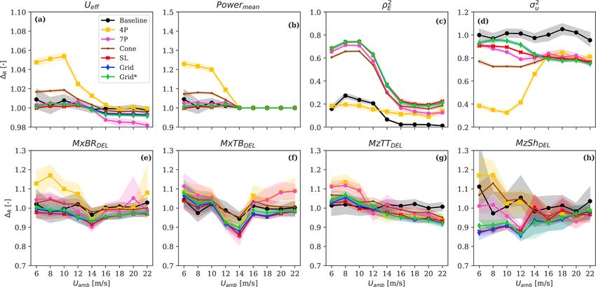
D. Conti et al.: Wind turbine load validation in wakes using wind field reconstruction techniques                               843

cumvent the DWM model’s assumption to consider wakes                    We use two sets of random turbulence field realizations,
passive tracers (Madsen et al., 2010), while reconstructing          which we denote as set A and set B. These turbulence fields
the actual observed inflow at a high spatial and temporal res-       are generated using the model by Mann (1994); thus, they
olution.                                                             are defined as zero-mean, homogeneous, uniform-variance
   The second approach reconstructs wake deficit character-          Gaussian random fields. We simulate DWM model-based
istics including wake meandering by fitting a bivariate Gaus-        wake fields using turbulence realizations from set A, which
sian shape function to lidar retrievals and superimposes these       we denote as the target fields (see the rectangular black boxes
deficits on a random realization of the Mann turbulence field.       in Fig. 1). In contrast, the DWM model-based wake fields us-
This approach intends to minimize errors in wake deficit rep-        ing turbulence field realizations from set B are denoted as the
resentations and introduce the observed wake meandering              baseline (see the rectangular blue boxes in Fig. 1). Since the
path directly into the simulations. Both lidar-based wake field      turbulence fields from set A and set B have the same turbu-
reconstruction techniques can potentially decrease the mod-          lence characteristics, as they are generated using the same
eling and statistical uncertainty inherent to the DWM model,         Mann parameters, but are statistically independent (i.e., the
thus predicting accurate power productions and loads.                resulting wind fields time series are uncorrelated), we expect
   We evaluate these lidar-based wake field reconstruction           that the outcomes of load simulations with set A and set B
techniques in a tailored designed numerical framework that           will have the same statistical properties but will not be corre-
simulates a nacelle-mounted lidar scanning the synthetic             lated (Dimitrov and Natarajan, 2017).
wake fields generated with the DWM model. The main ob-                  Hence, the result of a one-to-one comparison of load statis-
jective of this study is to verify that nacelle-mounted lidar        tics between the baseline and the target simulations is a direct
measurements incorporated into wake field reconstruction             measure of the statistical uncertainty (i.e., load scatter) that
methods improve the accuracy of power and load predictions           originates from both the random Mann-based turbulence re-
when compared to wake field reconstruction using engineer-           alizations and the stochastic meandering process inherent to
ing wake models alone.                                               the DWM model. In a traditional load validation analysis, the
   The work is structured as follows. In Sect. 2, we briefly         target loads will be the measured loads, whereas the baseline
formulate the load validation procedure. Section 3 introduces        loads will be the loads resulting from aeroelastic simulations
the methodology including the Mann spectral tensor model             using turbulence fields with the same properties as the mea-
(Sect. 3.1) and the DWM model (Sect. 3.2). Section 3.3 de-           sured inflow conditions (IEC, 2015).
scribes the virtual lidar simulator and the analyzed scanning           To evaluate the lidar-based approaches, we use a virtual
configurations. The wake field reconstruction techniques are         lidar simulator that scans the target wake fields and, through
formulated in Sect. 3.4. The results are provided in Sect. 4,        our proposed wake field reconstruction technique, incorpo-
including the uncertainty analysis of the lidar-reconstructed        rates these samples in a random turbulence field realization
fields in Sect. 4.1; a detailed analysis of the load validation      from set B (see Fig. 1). This numerical approach intends to
results in Sect. 4.2; and the effects of the lidar specifications,   imitate what we would eventually do when nacelle lidar mea-
e.g., probe volume size and sampling frequency, and those            surements within wakes are available for load predictions.
related to the atmospheric inflow conditions on the load pre-           Further, by incorporating lidar retrievals in the wind field
diction accuracy in Sect. 4.3. The last two sections are ded-        reconstruction technique, we expect to reduce the amount of
icated to the discussion of the findings and the conclusions         statistical uncertainty as the load time series resulting from
from the study.                                                      this approach will have greater similarity with the load time
                                                                     series based on the target turbulence fields. Therefore, this
                                                                     procedure allows us to quantify the uncertainty in load pre-
2   Problem formulation                                              dictions that results from lidar-reconstructed wake fields (see
                                                                     the red elements in Fig. 1) against the target and, at the same
The design load cases (DLCs) and load verification proce-            time, to compare the associated statistical uncertainty with
dure for wind turbines operating in wakes are described in           that of the baseline. To summarize, the following load simu-
the IEC standards (IEC, 2015, 2019). The present work cov-           lation cases are defined:
ers the analysis of fatigue loads of wind turbines operating
in wakes (see IEC 61400-1, DLC1.2). We apply the one-to-               – Target. These are DWM model-based wake fields im-
one load validation procedure of IEC 61400-13 (IEC, 2015),               posed on random turbulence field realizations from
which consists of comparing simulated and targeted (e.g.,                set A.
measured) load statistics to assess the accuracy of aeroelas-          – Baseline. These are DWM model-based wake fields
tic simulations. As we carry out the load validation analy-              imposed on random turbulence field realizations from
sis numerically, we define a tailored designed load validation           set B.
procedure, inspired by the approach of Dimitrov and Natara-
jan (2017) and illustrated in Fig. 1. The DTU 10 MW wind               – Constrained simulations (CSs). These are lidar-
turbine (Bak et al., 2013) is used as reference in this study.           reconstructed wake fields, where lidar virtual measure-

https://doi.org/10.5194/wes-6-841-2021                                                       Wind Energ. Sci., 6, 841–866, 2021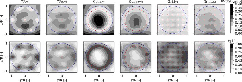
844                          D. Conti et al.: Wind turbine load validation in wakes using wind field reconstruction techniques

Figure 1. An illustration of the numerical framework utilized to reconstruct wake fields through the DWM model and our proposed lidar-
based wake field reconstruction techniques (i.e., the constrained simulations, CSs, and the wake deficit simulations, WDSs). Further, this
framework allows quantifying the uncertainty in power and load predictions resulting from aeroelastic simulations with the DWM model-
based and lidar-based wake fields. More details can be found in the text.

      ments of the target fields are incorporated as constraints       by reconstructing wake fields with stronger similarities to the
      to random turbulence field realizations from set B.              actual inflow.
  – Wake deficit simulations (WDSs). These are lidar-
    reconstructed wake fields, where lidar virtual measure-            3     Methodology
    ments of the target fields are fitted to a wake deficit
    shape function to compute wake deficits, which are then            3.1    Mann turbulence spectral model
    superimposed onto random turbulence field realizations
    from set B.                                                        The time-domain aeroelastic simulations require input of a
                                                                       three-dimensional turbulence field that mimics atmospheric
   The load validation comprises a large number of simula-             turbulence (Dimitrov et al., 2017). For this purpose, the IEC
tions (we use 18 random turbulence field realizations for each         61400-1 recommends, inter alia., the Mann uniform shear
individual 10 min statistic of the inflow wind) to quantify the        spectral tensor model (Mann, 1994) or the Kaimal model
statistical uncertainty in power and load predictions under in-        (Kaimal et al., 1972). The turbulence spectral properties of a
flow conditions measured at a site. More details on the load           three-dimensional homogeneous wind field are described by
validation analysis are provided in Sect. 4.2. Eventually, we          the spectral velocity tensor 8ij (k) (Kristensen et al., 1989):
quantify the load uncertainties of the baseline and CS and
WDS methods by comparison to the loads of the target sim-                            1
                                                                                            Z
ulations, and we define two main criteria to evaluate the pro-         8ij (k) =                Rij (r) exp(−ik · r)dr,               (1)
                                                                                   (2π )3
posed approaches:
                                                                       which is the Fourier transform of the covariance tensor
  I. The bias (here defined as the mean ratio between
                                                                       Rij (r); r = (x, y, z) is the spatial separation vector defined
     simulated and target loads) obtained with the lidar-
                                                                       in a right-handed coordinate system such that the longitu-
     reconstructed CSs and WDSs is equal to that obtained
                                                                       dinal component of the wind field (u) is in the x direction,
     with the baseline.
                                                                       y and z are the directions of the transverse components (i.e.,
 II. The statistical uncertainty (here defined as the stan-            the v- and w-velocity components), and k = (k1 , k2 , k3 ) is the
     dard deviation of the ratio between simulated and tar-            vector with the wavenumbers in the (x, y, z) directions.
     get loads) derived with the lidar-reconstructed CSs and              The model by Mann (1994) (hereafter referred to as the
     WDSs is lower than that obtained with the baseline.               Mann model), assumes neutral atmospheric conditions and
                                                                       defines the spectral tensor as a function of three input pa-
   Provided that these criteria are satisfied, the proposed            rameters: αk  2/3 is a product of the spectral Kolmogorov
lidar-based wake field reconstruction techniques will pro-             constant αk and the turbulent energy dissipation rate ; 0
duce (I) power and load predictions in wakes that are sta-             is a parameter describing the anisotropy of the turbulence,
tistically unbiased compared to the DWM model results and              and L is a length scale proportional to the size of turbulence
(II) a reduced statistical uncertainty in power and load predic-       eddies. From the spectral tensor, the cross spectra between
tions compared to the DWM model results, which is achieved             two points located in a y–z plane and separated by a distance

Wind Energ. Sci., 6, 841–866, 2021                                                              https://doi.org/10.5194/wes-6-841-2021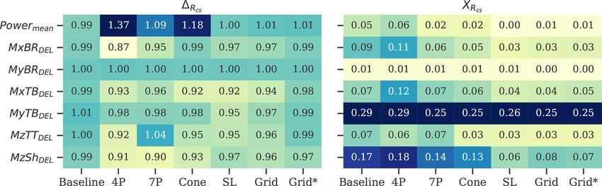
D. Conti et al.: Wind turbine load validation in wakes using wind field reconstruction techniques                                           845

(1y , 1z ) are calculated numerically by                                   tor (Madsen et al., 2010) as
                        ZZ
χij (k1 , 1y , 1z ) =        8ij (k, αk  2/3 , L, 0)                                                               ∂ 2 Udef (y, z)
                                                                           kmt (y, z) = | 1 − Udef (y, z) | km1 +                   km2 ,   (4)
                                                                                                                         ∂y∂z
                        × exp(ik2 1y + ik3 1z )dk2 dk3 .             (2)
                                                                           where Udef is the axisymmetric velocity deficit in the MFoR
Further, by inverse Fourier transforming the cross spectrum                (see also Fig. 2a) and km1 and km2 are calibration constants
χij , we can derive the auto- and cross-correlation structure              (Madsen et al., 2010). The two-dimensional spatial distri-
of the turbulence field (Dimitrov and Natarajan, 2017) as                  bution of kmt is shown in Fig. 2b. As wake turbulence is
                        Z                                                  both highly isotropic and characterized by a reduced turbu-
Rij (1x , 1y , 1z ) ∝        χij (k1 , 1y , 1z ) exp(ik1 1x )dk1 .   (3)   lence length scale compared to that of the ambient turbulence
                                                                           (Madsen et al., 2005), kmt of Eq. (4) scales the residual field
                                                                           of a Mann-generated turbulence field with a standard devi-
                                                                           ation of the longitudinal wind component equal to 1 m s−1
3.2   Dynamic wake meandering model                                        (IEC, 2019), assuming isotropic turbulence, i.e., 0 = 0, and
The DWM model is an engineering wake model that simu-                      a small turbulence length scale (L ≈ 10 %–25 % of the am-
lates wind field time series and includes three components:                bient turbulence length scale) (Madsen et al., 2010).
a quasi-steady velocity deficit, the wake-added turbulence,                   The wake meandering is assumed to be governed by the
and the wake meandering (Madsen et al., 2010). Figure 2                    atmospheric turbulent structures of the order of two rotor di-
illustrates these wake feature components qualitatively. The               ameters (D) or larger (Madsen et al., 2010). This assump-
DWM model assumes wakes as passive tracers displaced in                    tion was verified using lidar observations of wakes (Bingöl
the lateral and vertical directions by the large eddies in the             et al., 2010; Trujillo et al., 2011). Thus, the simulated wake
atmospheric flow. Further, the quasi-steady wake deficits are              meandering time series is obtained by low-pass filtering at-
advected in the stream-wise direction adopting Taylor’s as-                mospheric turbulence fluctuations (i.e., v- and w-velocity
sumption of frozen turbulence (Madsen et al., 2010). This                  components measured from a local mast or lidar or alter-
set of assumptions allows decoupling the wake deficit and                  natively simulated by the Mann model) by a cutoff fre-
wake-added turbulence components from the wake meander-                    quency fcut,off = Ūamb /(2D), which excludes contributions
ing model (Larsen et al., 2007). Hence, the three compo-                   from smaller eddies to the meandering dynamics (Larsen
nents of the DWM model are computed separately and sub-                    et al., 2008).
sequently superposed on random homogeneous turbulence                         As a result, the wake field simulated by the DWM model
field realizations (e.g., generated using the Mann model) to               can be seen as a cascade of quasi-steady velocity deficits
produce three-dimensional wake field time series that are in-              that meander in the lateral and vertical directions and are ad-
put into aeroelastic simulations (Larsen et al., 2013; Keck                vected downstream by the mean wind speed of the inflow
et al., 2014).                                                             using Taylor’s assumption. These wake features are super-
   The velocity deficit definition is based on the work of                 posed on stochastic homogeneous turbulence field realiza-
Ainslie (1986, 1988), who applied a thin shear-layer approx-               tions to generate wake fields time series that are then input
imation of the Navier–Stokes equations and a simple eddy                   into aeroelastic simulations (see Fig. 2c).
viscosity formulation. The wake deficit expansion and recov-                  Mathematically, a three-dimensional synthetic wake flow
ery downstream of the generating turbine are driven by the                 field compliant with the DWM model formulation can be de-
turbulent mixing occurring due to the ambient turbulence and               fined by a linear superposition of the ambient wind field and
the turbulence generated by the wake shear field itself (Mad-              two inhomogeneous turbulence terms as
sen et al., 2010; Keck et al., 2014, 2015). For a given wind
turbine aerodynamic rotor design, a 10 min average inflow                  UDWM (x, y, z) = Ūamb (z) + u0i,Kdef (x, y, z)
wind speed (Ūamb ), and ambient turbulence intensity (TIamb ),
                                                                                           + u0j,Kturb (x, y, z),                           (5)
the DWM model calculates a two-dimensional quasi-steady
velocity deficit defined in the meandering frame of reference
(MFoR), which is a coordinate system with its origin in the                where Ūamb (z) is the ambient wind speed including the atmo-
center of symmetry of the deficit, as shown in Fig. 2a. Here,              spheric vertical wind shear profile, u0iKdef (x, y, z) is a resid-
we use the numerical scheme of the standalone DWM model                    ual turbulence field with imposed wake deficits that follow
(Liew et al., 2020; Larsen et al., 2020) to compute the quasi-             the meandering path and u0j,Kturb is a second turbulence field
steady velocity deficit.                                                   modeling wake-added turbulence effects. Adopting Taylor’s
   The wake-added turbulence originating from the break-                   assumption, the wake field can be described by the spatial
down of tip vortices and from the shear of the velocity deficit            vector solely; thus, the time variable is disregarded in Eq. (5).
is accounted for by a semi-empirical turbulence scaling fac-               The subscripts i and j indicate two random and uncorrelated

https://doi.org/10.5194/wes-6-841-2021                                                              Wind Energ. Sci., 6, 841–866, 2021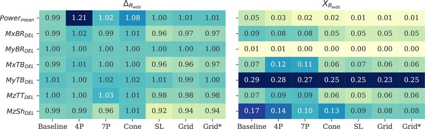
846                            D. Conti et al.: Wind turbine load validation in wakes using wind field reconstruction techniques

Figure 2. Qualitative representation of the three wake components predicted by the DWM model, including an axisymmetric quasi-steady
velocity deficit, which is defined as the local wind speed U divided by the ambient wind speed Ūamb (a); a wake-added turbulence scaling
factor, kmt (b), that assumes zero values outside of the wake region; and the meandering of the quasi-steady wake deficit superposed on a
random homogeneous turbulence field realization (c). The red marker identifies the wake center position, and the solid red line identifies the
wake center’s trajectory along the longitudinal x and lateral y coordinate. The wake also meanders in the vertical direction (not shown). The
wake features are computed for an ambient inflow characterized by Ūamb = 6 m s−1 and a turbulence intensity of TIamb = 8 %.

turbulence field realizations. The u0i,Kdef field is computed as           The lidar simulator derives the line-of-sight (LOS) veloci-
                                                                           ties at each scanning location by transforming the u-, v-, and
u0i,Kdef (x, y, z) = Ūamb (z)(1 − Kdef (x, y, z)) + u0i (x, y, z)         w-velocity components of the synthetic turbulence field into
                                                                           a LOS coordinate system. To simulate the probe volume of
                    − Ūamb (z),                                     (6)
                                                                           the lidars, a Gaussian weighting function W (F, r) is imposed
                                                                           along the LOS coordinate r and centered at the focal distance
where Kdef (x, y, z) denotes the DWM model-based wake
                                                                           F:
deficit time series including a pre-computed stochastic me-
andering path, and u0i is a random homogeneous turbulence
                                                                                       Z
                                                                           VLOS,eq = VLOS (r)W (F, r)dr.                               (8)
field realization from the Mann model with the same Mann
parameters as those of the ambient wind field. Note that
Kdef (x, y, z) assumes values equal to unity when wake losses              The u velocity is computed from the projection of VLOS,eq
are not present. The Mann parameters, αk  2/3 , L, and 0,                 onto the longitudinal axis; i.e., the v- and w-velocity compo-
are derived, e.g., from fitting the observed free-stream tur-              nents are neglected in the field reconstruction (Schlipf et al.,
bulence velocity spectra to the Mann model with the use of                 2013; Simley et al., 2013). This assumption leads to
pre-computed lookup tables to speed up the fitting procedure                           VLOS,eq
(Peña et al., 2017). The wind field formulation of Eqs. (5)                ulidar =               ,                                       (9)
                                                                                      cos φ cos θ
and (6) is consistent with the domain of wind fields typically
input into aeroelastic simulations (Larsen and Hansen, 2007).              where φ is the elevation and θ the azimuth angle of the scan-
Finally, u0j,Kturb is obtained as                                          ning pattern, which refer to the rotations about the y and
                                                                           z axes, respectively. Neglecting the v- and w-velocity com-
u0j,Kturb (x, y, z) = u0j (x, y, z)Kmt (x, y, z),                    (7)   ponents introduces uncertainty into the wind field reconstruc-
                                                                           tion. However, the opening angles (φ, θ ) relative to the scan-
where Kmt (x, y, z) denotes a time series of turbulence’s scal-            ning configurations of our work reach a maximum of 35◦
ing factors computed from Eq. (4) including a pre-computed                 (see Sect. 3.3.1); thus, the errors introduced by Eq. (9) are
stochastic meandering path and u0j is a random homogeneous                 marginal (Simley et al., 2013). Other sources of uncertainty
turbulence field with σu = 1 m s−1 , 0 = 0, and L = 10 % of                in the radial velocity estimation inherent to lidars, e.g., from
the ambient turbulence length scale (Madsen et al., 2010;                  the optics and internal signal processing, are accounted for
IEC, 2019).                                                                by adding Gaussian white noise. Here we add noise at a level
                                                                           that results in a signal-to-noise ratio of −20 dB as in Pettas
3.3   Lidar simulator
                                                                           et al. (2020). We do not investigate the sensitivity of the noise
                                                                           level in the present work.
We use the lidar simulator developed within the ViCon-                        The lidar simulator can mimic any arbitrary scanning pat-
DAR open-source numerical framework to virtually replicate                 tern and includes a time lag between each lidar-sampled mea-
lidar measurements (https://github.com/SWE-UniStuttgart/                   surement to resemble the scanning frequency (see Fig. 3). In
ViConDAR, last access: 22 April 2021) (Pettas et al., 2020).               the present study, the virtual lidar data are computed from the

Wind Energ. Sci., 6, 841–866, 2021                                                                https://doi.org/10.5194/wes-6-841-2021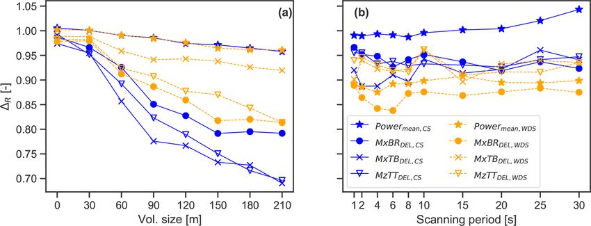
D. Conti et al.: Wind turbine load validation in wakes using wind field reconstruction techniques                                  847

                                                                       sample much faster at a given range but need to refocus in
                                                                       order to change the sampling range. In the present paper,
                                                                       we only consider a single focusing range that is achievable
                                                                       with both lidar technologies. Further, a time lag between each
                                                                       sampling beam is simulated to mimic lidars’ sampling fre-
                                                                       quency.
                                                                          Although we do not optimize the scanning patterns, we use
                                                                       scan radii (defined as the radius between hub height and the
                                                                       location of the scanned points) of about 70 %–80 % of the
                                                                       rotor radius to estimate wind field characteristics based on
                                                                       previous recommendations (Dimitrov and Natarajan, 2017;
                                                                       Simley et al., 2018). Thus, we define the 4P, 7P, and Cone
                                                                       patterns accordingly as shown in Fig. 4. The SL trajectory is
                                                                       scaled to cover the full rotor area, and the positions over the
Figure 3. An illustration of the virtual lidar simulator setup run
                                                                       plane of measurement are separated by 29 m in both vertical
for 175 s with simulated time lag. The wind turbine is sketched by     and transverse directions for the Grid pattern.
the solid black lines; the nacelle-mounted lidar is represented by a      A preview distance of 0.7D (≈ 125 m) is assumed. Note
square blue marker measuring upstream of the turbine. The trajec-      that increasing the preview distance reduces the errors caused
tory of the scanning beam is shown by discrete red dots.               by the cross-contamination effects of the v and w compo-
                                                                       nents and reduces the induction effects but raises errors due
                                                                       to the wind evolution (Simley et al., 2012). These effects
synthetic wake flow fields generated using the DWM model.              are not investigated in detail in this work, as we use DWM
These wind fields are time series of the u-, v-, and w-velocity        model-based wake fields as target, which do not include in-
components defined over a turbulence box with a grid size of           duction effects or turbulence evolution as Taylor’s assump-
8192×32×32 (x×y×z). A spatial resolution of 6.5 m is used              tion is applied.
for the grid in the rotor plane, which leads to a turbulence              We assume a 2 s scan period for all the simulated configu-
box with dimensions of 208 m × 208 m in both lateral and               rations, which refers to the time required for a beam to com-
vertical directions (y × z). The spatial resolution dx on the          plete the full pattern. Given the finite resolution of the syn-
x axis depends on the simulated ambient wind speed at hub              thetic turbulence boxes (i.e., 6.5 m in both lateral and vertical
height: dx = (Ūamb Tsim )/8192, where Tsim is the simulation          directions), the Cone and SL scanned locations are binned
time in seconds. These dimensions ensure an adequate tur-              within the box grid, as reported in Table 1.
bulence field for a 10 min wind field simulation over a large             A probe volume with an extension of 30 m in the LOS
rotor and a space–time resolution such that the probe volume           direction is assumed for all the analyzed patterns, which is
effects can be captured by the virtual lidar (Dimitrov et al.,         comparable with the current CW lidar technology measur-
2017; Pettas et al., 2020).                                            ing at distances beyond 120 m (Peña et al., 2015). Further, a
                                                                       30 m probe length is commonly used to model pulsed lidars
3.3.1   Lidar scanning strategies                                      (Schlipf, 2016). Here, we define the probe volume’s length
                                                                       as the standard deviation of the Gaussian weighting function
To evaluate currently available nacelle lidars’ ability to per-        for convenience. Typically, Gaussian weighting functions are
form wake characterization, we select a few standard scan-             used to model pulsed lidars, whereas Lorentzian functions
ning configurations and use them to perform load valida-               are used for CW lidars (Mann et al., 2010). Additionally, we
tion within wakes. These are a four-beam lidar (4P) (Held              define a case (Grid∗ ) that neglects probe volume averaging
and Mann, 2019a, b); an extended configuration with seven              effects (see Table 1).
beams, six arranged at the corner of a hexagon and a cen-
tral beam (7P) (Pettas et al., 2020); the conical scanning
lidar (Cone) (Medley et al., 2014; Borraccino et al., 2017;            3.4   Wake field reconstruction techniques
Peña et al., 2017); the SpinnerLidar (SL) (Peña et al., 2019;
Doubrawa et al., 2019); and a general grid pattern (Grid) cov-         By defining the DWM model-based wake flow fields as the
ering the full turbulence box (see Fig. 4).                            target fields, the underlying assumptions on which we define
   The lidar simulator is assumed to scan the selected pat-            the lidar-based wake field reconstruction techniques are as
terns at the same single range upwind of the rotor. Pulsed             follows:
and continuous-wave (CW) lidar technologies apply different
approaches at scanning multiple ranges (Peña et al., 2017).              1. The ambient wind conditions are known, including
Pulsed lidars can scan multiple ranges along the LOS simul-                 Ūamb (z), the atmospheric turbulence intensity (TIamb ),
taneously within a single sample, while CW lidars typically                 and the atmospheric stability conditions (here implic-

https://doi.org/10.5194/wes-6-841-2021                                                         Wind Energ. Sci., 6, 841–866, 2021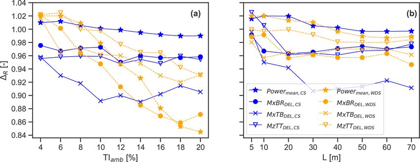
848                            D. Conti et al.: Wind turbine load validation in wakes using wind field reconstruction techniques

Figure 4. Selected lidar scanning patterns for the load analysis. The red markers indicate the scanned locations, and the black dots in the
background define the spatial resolution of the turbulence box. The rotor diameter is shown as a solid black line.

Table 1. Technical properties of the simulated lidar scanning configurations. Note that the Cone and SL measurements are binned according
to the spatial resolution of the synthetic turbulence fields, thus leading to a reduction in the simulated scanning positions.

                 Scanning                 Measurements/           Sampling           Scan     Measurements/      Probe volume
                 configuration          scan (binned) [–]    frequency [Hz]     period [s]       10 min [–]           size [m]
                 4P                                     4                  2             2              1200                 30
                 7P                                     7                3.5             2              2100                 30
                 Cone                            100 (30)                 50             2              9000                 30
                 SpinnerLidar (SL)               400 (93)                200             2             27 900                30
                 Grid                                  49                 25             2             14 700                30
                 Grid∗                                 49                 25             2             14 700                 0

      itly prescribed through the Mann parameters – αk  2/3 ,             analytical wake models; however, in this study, the wake
      L, and 0).                                                           characteristics are extracted directly from the lidar observa-
                                                                           tions rather than from a physically based deficit formulation.
  2. The lidar-based wake fields are reconstructed by incor-
                                                                           Eventually, wind turbine responses are mainly affected by
     porating lidar observations (e.g., in the form of con-
                                                                           the mean wind speed in the longitudinal direction (u veloc-
     straints or lidar-fitted velocity deficits) into a zero-mean,
                                                                           ity) and its variance (Dimitrov et al., 2018), while the effects
     homogeneous, and random Gaussian turbulence field
                                                                           of the v and w turbulence are generally marginal (Dimitrov
     generated by the Mann spectral tensor model.
                                                                           and Natarajan, 2017).
  3. The induction effects on lidar measurements are ne-
     glected, and Taylor’s frozen turbulence hypothesis is as-             3.4.1    Constrained Gaussian field simulations
     sumed.
                                                                           The algorithm for applying constraints on a zero-mean, ho-
  4. Only the u-velocity fluctuations are reconstructed from               mogeneous, and isotropic Gaussian random field was devel-
     the lidar measurements of the target wake fields.                     oped in Hoffman and Ribak (1991) and extended to Mann-
   The corresponding random turbulence field realizations                  generated turbulence fields for aeroelastic simulations in
from set A (used for the target fields) and set B have sim-                Nielsen et al. (2003) and Dimitrov and Natarajan (2017). The
ilar spectral properties; however, these fields only describe              algorithm uses a set of constraints that are here derived from
the turbulence structures of the ambient wind field. The li-               a virtual lidar simulator and an unconstrained random tur-
dar measurements of the wake field, combined with the wake                 bulence realization generated with the Mann spectral tensor
field reconstruction approach, should recover all the infor-               model.
mation regarding the wake characteristics, including veloc-                   Following the notation in Dimitrov and Natarajan (2017),
ity deficits, wake-added turbulence, and meandering in lat-                we denote g̃(r), where r = (x, y, z) is the spatial separa-
eral and vertical directions. Further, the first assumption is             tion vector, an unconstrained random turbulence realization.
no longer needed if a second instrument is deployed at the                 The spectral property of g̃(r) at each discrete lateral and
site measuring the ambient conditions, for example, using                  vertical separation of the turbulence box can be computed
a mast or a nacelle-mounted lidar (Borraccino et al., 2017;                from the Mann model in Eq. (2), given a set of parame-
Peña et al., 2017).                                                        ters (αk  2/3 , L, 0). We denote a set of constraints as H =
   The second and third assumptions are inherent in the mod-               {hi (r)|ri = ci , i, . . ., M}, where each constraint is a measured
eling approach and limitations of the DWM model and other                  value of the wind speed for a particular spatial location r

Wind Energ. Sci., 6, 841–866, 2021                                                               https://doi.org/10.5194/wes-6-841-2021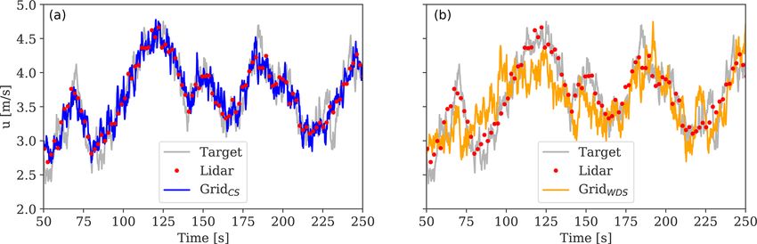
D. Conti et al.: Wind turbine load validation in wakes using wind field reconstruction techniques 849
and M is the total number of constraints (i.e., the number of deficit is defined as the difference between the ambient wind
scanned points within a 10 min period). Note that the con- speed and that inside the wake as
straints are defined as a residual wind field; thus, we remove
the mean ambient wind speeds from the lidar measurements Ūamb (z) − ulidar (x, y, z)
Udef (x, y, z) = , (13)
of Eq. (9), i.e., ci (r i ) = ulidar (r i ) − Ūamb (r i ), which are the Ūamb (z)
values that are input into the algorithm.
The objective of the algorithm is to define a turbulence where Ūamb (z) is assumed to be known and the lidar mea-
field g(r), subjected to the constraints in H that main- surements in the wake (ulidar ) are sampled by the lidar simu-
tain the covariance and coherence properties of the uncon- lator using Eq. (9). Following the procedure of Trujillo et al.
strained field g̃(r). As demonstrated in Dimitrov and Natara- (2011), a bivariate Gaussian shape is used to describe the ve-
jan (2017), the unknown points of the field can be defined locity deficit flow field as
by maximizing their conditional probability distribution on A
the constraint set H. We define the residual field ξ (r) = Kdef,Gau (y, z) =
2π σwy σwz
g(r) − g̃(r), which is the difference between the constrained " !#
and unconstrained fields. This residual field is also a random 1 (yi − µy )2 (zi − µz )2
× exp − 2
+ 2
,
Gaussian field, where its values at the constraint locations 2 σwy σwz
are known: ξ (r i ) = ci (r i ) − g̃c (r i ). The values of the resid- (14)
ual field at unknown locations can be derived as (Dimitrov
and Natarajan, 2017) where (µy , µz ) define the wake center location; (σwy , σwz )
are width parameters of the wake profile in the y and z direc-
ξ̄ (r) = hξ (r)|Hi = ζ (r)Z−1 (H − g̃c (r)), (10) tions, respectively; (yi , zi ) denote the spatial location of the
LOS; and A is a scaling parameter dictating the depth of the
where h.i denotes ensemble averaging, ζ (r) is a vector of wake. A least-squares method is applied to fit the measured
cross correlations between the constraints and the field, and wind speed deficits from Eq. (13) to the bivariate Gaussian
Z is the symmetric correlation matrix of the constraints set. function in Eq. (14).
Both ζ (r) and Z can be computed from Eq. (3). Eventually, The optimal wake deficit parameters (µy , µz , σwy , σwz , A)
any constrained realization can be written as a sum of the are obtained for each completed scanning period (i.e., ∼ 2 s
unconstrained field and the mean of the residual field as as described in Table 1), resulting in approximately 300 lidar-
reconstructed deficits within a 10 min period. Finally, these
g(r) = g̃(r) + ζ (r)Z−1 (H − g̃c (r)). (11) lidar-fitted wake deficits are superimposed on a random ho-
mogeneous turbulence field realization from set B, as shown
By denoting u0CS,B,i = g(r) as the constrained turbulence
in Fig. 1. A preliminary analysis showed that wide turbulence
field that incorporates lidar measurements into a random tur-
boxes (208 m×208 m) can present large turbulence structures
bulence realization i from set B (see Fig. 1), we can derive
within, i.e., broad regions across the box characterized by
the reconstructed wake flow field to be input into aeroelastic
low wind speeds, whose sizes can alter the depth and width
simulations as
properties of the lidar-fitted wake deficits in Eq. (14). As a
UCS (x, y, z) = Ūamb (z) + u0CS,B,i (x, y, z). (12) result, the wake properties of the reconstructed field can con-
siderably deviate from the actual imposed wake characteris-
Note that the fidelity of the reconstructed wind field will de- tics.
pend on the accuracy of the nacelle lidar measurements used To compensate for these deviations and considering that
to characterize the wake field. the DWM model-based wake fields can be defined as a lin-
ear summation of the ambient wind field Ūamb scaled by the
wake deficit function Kdef and a random homogeneous tur-
3.4.2 Wake deficit superposition simulations
bulence realization term u0i , as reported in Eq. (6), we refor-
The wake deficit superposition (WDS) approach assumes mulate the least-squares minimization problem as
that velocity deficits can be described by a bivariate Gaussian
shape function, which is fitted based on lidar measurements X
0def = Udef (ym , zn )
of the target wake flow field. Several studies have demon-
mn
strated the viability and robustness of the Gaussian curve fit-
2
ting to track wake deficit displacements in the far-wake re- Ūamb − (Ūamb (z)(1 − Kdef,Gau (ym , zn |µy , µz , σwy , σwz , A))
+u0B,i (y, z))
gion (Trujillo et al., 2011; Reinwardt et al., 2020).
− ,
(15)
Ūamb (z)
In our study, the wake shape function not only tracks
the wake meandering but also is used to quantify the depth
and width of the wake at each quasi-instantaneous scan per- where subscripts (m, n) indicate data points within the scan-
formed by the lidar. Traditionally, the normalized velocity ning configuration; the second term on the right-hand side
https://doi.org/10.5194/wes-6-841-2021 Wind Energ. Sci., 6, 841–866, 2021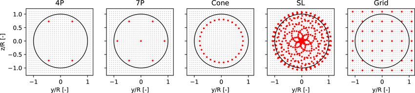
850 D. Conti et al.: Wind turbine load validation in wakes using wind field reconstruction techniques
defines the velocity deficit as in Eq. (13), in which the recon- information is included. Contrarily, ρE2 = 1 indicates that the
structed wake field is defined as Ūamb (1 − Kdef,Gau ) + u0B,i ; reconstructed time series is fully correlated with the target;
and u0B,i is the random homogeneous turbulence realiza- thus the two fields match completely.
tion from set B. Note that when wake losses are present, Figure 5 also shows the spatial distribution of ρE2 de-
(1 − Kdef,Gau ) will reduce the ambient wind speed, as ex- rived from the CS- and WDS-reconstructed fields, with the
pected. As the sampling frequency of the lidar is lower than 7P, Cone, and Grid configurations (see Table 1 for specifi-
the sampling frequency of the synthetic wind field, we in- cations). For this particular analysis, the turbine of interest
terpolate the fitted wake characteristics at each scan to the is located 5D downstream of the upstream turbine, where
whole turbulence field by applying a nearest-neighbor inter- D = 179 m is the diameter of the DTU 10 MW turbine, and
polation scheme. Finally, the reconstructed wake field input ambient conditions are characterized by Uamb = 6 m s−1 and
into aeroelastic simulations is defined by TIamb = 8 %. The inflow wind profile is defined by a power-
law model with a shear exponent of 0.2.
UWDS (x, y, z) = Ūamb (z)(1 − Kdef,Gau (x, y, z)) As shown in Fig. 5, the locations of the imposed con-
+ u0B,i (x, y, z), (16) straints are characterized by the lowest RMSE and highest
ρE2 . This effect is more pronounced for the CS results, as
where Kdef,Gau (x, y, z) is fitted using Eq. (15) for each com- the algorithm imposes the actual observations directly on the
pleted scan by the nacelle lidar. synthetic field. The RMSE would tend to zero if the length of
probe volume were neglected, the lidar’s sampling frequency
4 Results corresponded to the sampling frequency of the wind field,
and cross-contamination effects were compensated for. The
The results are divided into three parts. First, we assess RMSE increases (and ρE2 decreases) for spatial regions that
the accuracy of lidar-reconstructed wake fields against tar- are farther from the lidar’s beams. This occurs due to the co-
get fields in Sect. 4.1. Second, we carry out the load vali- variance structure of the unconstrained turbulence field, for
dation analysis in Sect. 4.2 and separately present the load which the unknown points are nearly uncorrelated with the
prediction uncertainty of the CS approach in Sect. 4.2.2 and imposed constraints.
that of the WDS approach in Sect. 4.2.3. A detailed analysis The errors introduced by the WDS fields are partly a con-
of the predicted load time series and load spectral properties sequence of an inaccurate estimation of the wake deficit char-
is conducted in Sect. 4.2.4 and 4.2.5. Finally, we evaluate acteristics (i.e., due to the limited spatial scanning configura-
the effects of both atmospheric turbulence conditions and the tion) and the small-scale turbulence structures contained in
selected lidar technical specifications on the load prediction the turbulence box. Finally, the results in Fig. 5 confirm that
accuracy in Sect. 4.3. the number of scanned positions by the lidar has a significant
impact on the reconstructed fields’ accuracy, affecting both
4.1 Uncertainty in reconstructed wake fields the mean and variance of the reconstructed u-velocity com-
ponent. Therefore, patterns that cover a larger region of the
In this section, we evaluate the accuracy of the lidar-
rotor lead to more accurate field representations (Dimitrov
reconstructed fields against the target fields. At first, we as-
and Natarajan, 2017; Pettas et al., 2020).
sess the accuracy of the reconstructed u-velocity time se-
In Fig. 6, we compare the lidar-reconstructed u-velocity
ries across the turbulence
q box,Pby computing the root mean time series extracted at hub height, using the Grid pattern,
square error, RMSE = 1/n ni (ỹi − ŷi )2 /ȳi , between the with the target observations derived at the same location.
lidar-reconstructed (ỹ) and target velocity (ŷ), where n = The target wake field is simulated with Uamb = 6 m s−1 and
8192 is the grid size of the box in the longitudinal direction, TIamb = 8 %. The time series of the virtual lidar measure-
normalized over the mean target velocity (ȳi ) at each grid ments is also shown. We find that both field reconstruction
point of the turbulence box. The normalized RMSE provides approaches can predict the reduced wind speed within the
a measure of the quality of the lidar-reconstructed fields with wake region and recover the details of the wind speed fluctu-
respect to the target fields; values closer to zero indicate a ations in the target field. However, uncertainty is introduced
high precision and accuracy (see Fig. 5, top row). due to the limited lidar sampling frequency, the probe vol-
Further, we compute the explained variance ratio across ume length (here assumed to be 30 m), and the adopted field
the turbulence box ρE2 = (cov(ỹ, ŷ)/σỹ σŷ )2 (i.e., the square reconstructing techniques. The results in Fig. 6 demonstrate
of Pearson’s correlation coefficient; Achen, 1982), which de- that incorporating lidar data directly in the reconstructed field
fines the proportion of the variance in the inflow field that is (i.e., the CS approach) leads to reproducing more accurate
transferred to the unconstrained turbulence field by impos- fields compared to the WDS approach.
ing the constraints (Dimitrov and Natarajan, 2017). As the In addition, we compute the power spectral density (PSD)
target and lidar-reconstructed fields are based on two sets of of the above-analyzed time series of u-velocity fluctuations
random uncorrelated turbulence field realizations (see sets A for a 10 min simulation and compare them in Fig. 7. We ob-
and B in Fig. 1), ρE2 ∼ 0 is expected across the box if no lidar serve that the PSD of the reconstructed fields is comparable
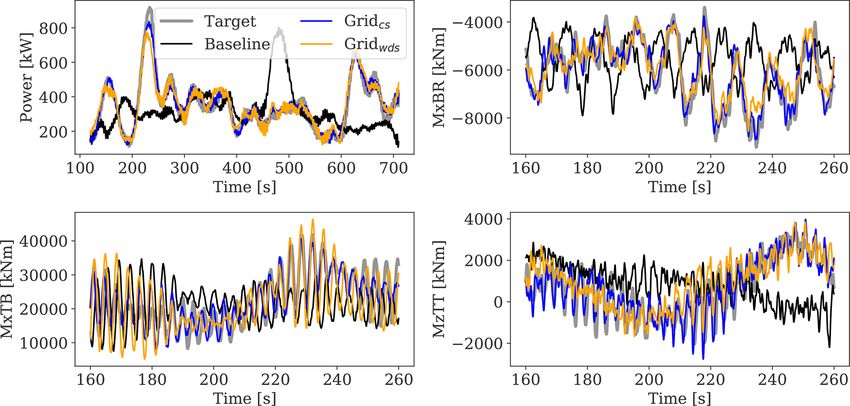
Wind Energ. Sci., 6, 841–866, 2021 https://doi.org/10.5194/wes-6-841-2021D. Conti et al.: Wind turbine load validation in wakes using wind field reconstruction techniques 851 Figure 5. Spatial distribution of the error inherent to the CS- and WDS-reconstructed fields for selected scanning configurations. The top row refers to the RMSE normalized over the target velocity at each grid point (Uwake ). The bottom row refers to the explained variance ratio. The red markers identify the centers of the lidar beam sampling volumes. The wind turbine rotor is shown with dotted blue line. Figure 6. Comparison between the target u-velocity time series at hub height (solid grey line) and the reconstructed field based on the CS approach (a) and WDS approach (b) extracted at hub height. The lidar data are shown with red markers. The target simulations are run with Uamb = 6 m s−1 and TIamb = 8 %. to that of the target for frequencies of up to ≈ 1 Hz, while the field, without the small-scale wake-added turbulence being energy spectral content at higher frequencies is attenuated. explicitly included. According to Larsen et al. (2008), the dominant frequency of the wake meandering is defined as fcut,off = Uamb /(2D) = 4.2 Load validation 0.016 Hz (∼ 62 s period) for Uamb = 6 m s−1 . As the lidar completes a full scan in 2 s, the large-scale wake meander- The DTU 10 MW reference wind turbine is used for the load ing dynamics are well captured. Further, as the wake mean- validation analysis (Bak et al., 2013). The load simulations dering is the main source of wake-added turbulence (i.e., u- are carried out using the aeroelastic code HAWC2 (Larsen component variance), the energy spectral content in the low- and Hansen, 2007) and inflow wind conditions measured frequency range is recovered, as shown in Fig. 7. from an offshore site, as described in Sect. 4.2.1. Note that The enhanced turbulent energy content of the target field we run the analysis based on offshore wind conditions, which within the high-frequency range (> 1 Hz) originates from are characterized by low turbulence; thus, wake effects are the small-scale wake-added turbulence (Madsen et al., 2010; more prominent. This work evaluates the load prediction ac- Chamorro et al., 2012). These effects are not fully recovered curacy at the main wind turbine structures, such as blades, in the reconstructed fields, mainly due to the lidar probe vol- shaft, and tower. Therefore, we neglect the modeling of the ume and limited sampling frequency and because the method offshore substructures and foundations, and we use the on- fits the lidar measurements to a standard Mann turbulence shore model of the DTU 10 MW. https://doi.org/10.5194/wes-6-841-2021 Wind Energ. Sci., 6, 841–866, 2021
852                          D. Conti et al.: Wind turbine load validation in wakes using wind field reconstruction techniques

Figure 7. Comparisons of the power spectra density (PSD) of the target u-velocity component measured at hub height with predictions
obtained by the CS field (a) and the WDS field (b). The dominant frequency of the wake meandering fcut,off ≈ 0.016 Hz, the rotational
frequency of the rotor and its harmonics (1P ≈ 0.1 Hz and 3P ≈ 0.3 Hz), and the Nyquist frequency of the lidar (≈ 0.25 Hz) are shown (see
text for more details).

   Following the load validation procedure illustrated in              4.2.1   Site conditions
Fig. 1, we quantify the uncertainty in power and load pre-
dictions resulting from the baseline, CSs, and WDSs against            Load simulations are carried out using site-specific observa-
results obtained with the target fields. The CSs and WDSs              tions collected from the FINO1 meteorological mast installed
are evaluated for the selected lidar configurations of Fig. 4,         at the German offshore wind farm Alpha Ventus. The wind
i.e., the 4P, 7P, Cone, SL, Grid, and Grid∗ patterns with the          farm is situated in the North Sea and about 45 km north of
parameters provided in Table 1. Two uncertainty indicators             the island of Borkum (Kretschmer et al., 2019). Data were
are defined to verify the load validation criteria I and II of         collected over a period of 3 years from 2011 to 2014, and
Sect. 2:                                                               their details can be found in Kretschmer et al. (2019).
  – Bias. 1R = E(ỹ)/E(ŷ).                                               In the present work, we only use wind speeds and tur-
                      p                                                bulence intensities measured under near-neutral conditions
  – Uncertainty. XR = h(ỹ/ŷ − E(ỹ)/E(ŷ))2 i.                       from a 90 m sonic anemometer installed at the mast. We
Here, the symbol E(.) denotes the mean value and h.i the               extract 10 min average turbulence values binned for wind
ensemble average, ŷ is the quantity of interest (i.e., power          speeds ranging between 6 and 22 m s−1 ; using wind speed
or load statistics) derived from the target simulations, and ỹ        bins with a 2 m s−1 bin width, we obtain nine bins with turbu-
corresponds to that produced by the reconstructed fields. We           lence intensities of 8, 7, 7, 6, 6, 6, 6, 5, and 5 %, respectively.
evaluate 1R and XR based on the resulting 10 min power                 These are the statistics of the ambient wind field that we use
and load statistics and provide results in Sect. 4.2.2 for the         as inputs for the load validation analysis.
CS fields and in Sect. 4.2.3 for the WDS fields.                          For each 10 min sample of the inflow wind, we use 18
   The analyzed wind turbine responses include mean power              turbulence field realizations (IEC 61400-1 recommends at
production levels (Powermean ) and fatigue loads. We use the           least 6 realizations), leading to 162 aeroelastic simulations
rainflow-counting algorithm to compute the 1 Hz damage                 for each scanning configuration analyzed. Simulations with
equivalent fatigue loads with a Wöhler exponent of m = 12              ambient wind speeds below 6 m s−1 are disregarded, as the
for blades and m = 4 for steel structures such as tower and            wind speed approaching the rotor drops below the turbine’s
shaft. Thus, we compute fatigue loads at the blade root                cut-in threshold due to wake deficit effects and the turbine
flapwise and edgewise moments, MxBRDEL and MyBRDEL ,                   shuts down.
and tower-bottom fore-aft and side–side, MxTBDEL and                      Note that the recorded turbulence estimates at Alpha Ven-
MyTBDEL , and torsional loads at the tower top (also referred          tus are considerably lower (by approximately a factor of
to as yaw moment), MzTTDEL , and the drivetrain, MzShDEL .             3) than values recommended by the low-turbulence IEC
   Furthermore, we quantify the accuracy of the recon-                 class C. Here, we perform the load validation analysis on
structed wake fields based on estimates of the rotor-effective         more realistic turbulence estimates characterizing offshore
wind speed (Ueff ), defined as the weighted sum of the u ve-           sites, since IEC class-C conditions would significantly atten-
locity measured across the rotor area, the explained variance          uate the wake-induced effects, as higher ambient turbulence
ratio ρE2 , and the u-velocity variance σu2 computed from the          leads to a faster recovery of the wake deficit.
reconstructed turbulence fields. Finally, a load time series              We use standard IEC-recommended turbulence parame-
and spectral analysis is conducted in Sect. 4.2.4 and 4.2.5.           ters for the Mann model (i.e., L = 29.4 m and 0 = 3.9; IEC,

Wind Energ. Sci., 6, 841–866, 2021                                                          https://doi.org/10.5194/wes-6-841-2021
You can also read