Merging the weak gravity and distance conjectures using BPS extremal black holes
←
→
Page content transcription
If your browser does not render page correctly, please read the page content below
Published for SISSA by          Springer
                                                                           Received: July 10, 2020
                                                                       Accepted: December 5, 2020
                                                                       Published: January 27, 2021

Merging the weak gravity and distance conjectures
using BPS extremal black holes

                                                                                                       JHEP01(2021)176
Naomi Gendlera and Irene Valenzuelab
a
  Department of Physics, Cornell University,
  East Avenue, Ithaca, NY 14853, U.S.A.
b
  Jefferson Physical Laboratory, Harvard University,
  Oxford Street, Cambridge, MA 02138, U.S.A.

    E-mail: ng434@cornell.edu, ivalenzuela@g.harvard.edu

Abstract: We analyze the charge-to-mass structure of BPS states in general infinite-
distance limits of N = 2 compactifications of Type IIB string theory on Calabi-Yau three-
folds, and use the results to sharpen the formulation of the Swampland Conjectures in the
presence of multiple gauge and scalar fields. We show that the BPS bound coincides with
the black hole extremality bound in these infinite distance limits, and that the charge-to-
mass vectors of the BPS states lie on degenerate ellipsoids with only two non-degenerate
directions, regardless of the number of moduli or gauge fields. We provide the numerical
value of the principal radii of the ellipsoid in terms of the classification of the singularity that
is being approached. We use these findings to inform the Swampland Distance Conjecture,
which states that a tower of states becomes exponentially light along geodesic trajectories
towards infinite field distance. We place general bounds on the mass decay rate λ of this
                                                                                                 √
tower in terms of the black hole extremality bound, which in our setup implies λ ≥ 1/ 6.
We expect this framework to persist beyond N = 2 as long as a gauge coupling becomes
small in the infinite field distance limit.

Keywords: Black Holes in String Theory, Superstring Vacua, Supergravity Models, Mod-
els of Quantum Gravity

ArXiv ePrint: 2004.10768

Open Access, c The Authors.
                                                        https://doi.org/10.1007/JHEP01(2021)176
Article funded by SCOAP3 .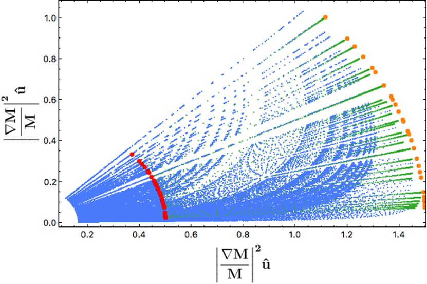
Contents
1 Introduction 1
2 Swampland conjectures in the presence of scalar fields 5
3 BPS states and extremal black holes in 4d N = 2 effective field theories 10
3.1 Review: N = 2 EFTs and BPS states in Calabi-Yau compactifications 10
3.2 BPS and extremality bounds in the infinite distance limit 12
JHEP01(2021)176
3.3 General structure of BPS charge-to-mass spectra 17
3.4 Example 1: one modulus case 20
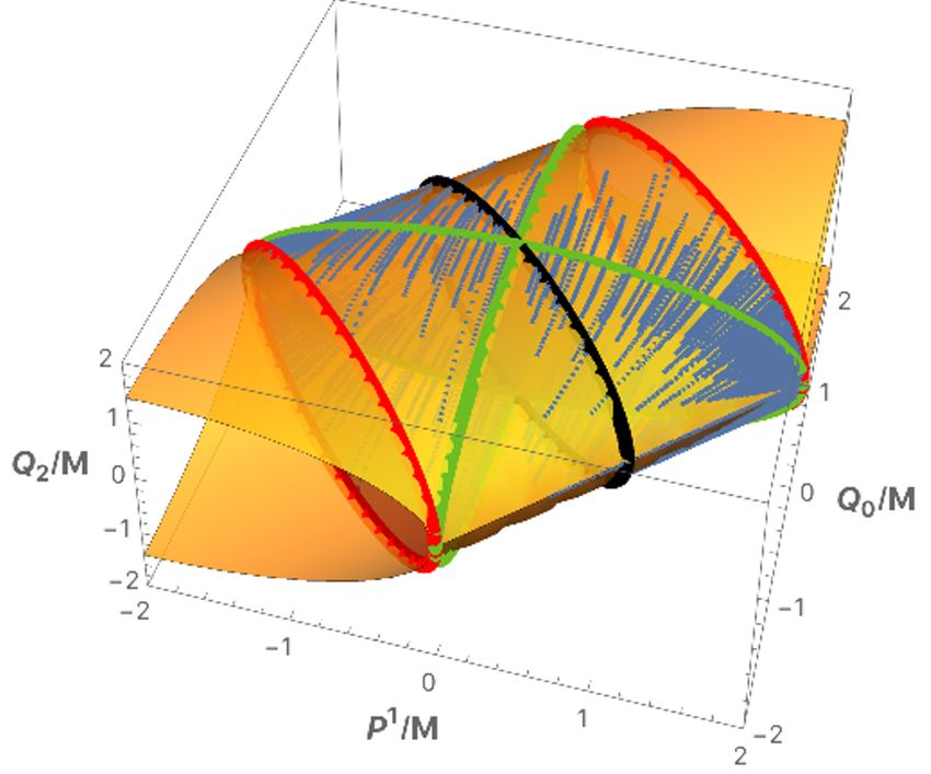
3.5 Example 2: two moduli case 23
3.6 Magnetic charge and dyons 26
4 General bounds in the asymptotic limit 27
4.1 Review: asymptotic Hodge theory techniques 28
4.2 Asymptotic form of the charge-to-mass ratio 32
4.3 General bounds on mass decay rate 35
4.4 Examples 40
5 Emergence and generalization to other setups 48
5.1 Non-BPS charges 49
5.2 Kaluza-Klein tower 53
5.3 Emergence and generality of our results 54
6 Conclusions 59
1 Introduction
The goal of the Swampland program (see [1, 2] for reviews) is to provide a set of criteria
that an effective field theory must satisfy in order to be a viable low-energy limit of a
UV-complete theory of quantum gravity. Of all the criteria that have been proposed for
this purpose, two of the most studied are the Swampland Distance Conjecture (SDC) [3]
and the Weak Gravity Conjecture (WGC) [4]. On the one hand, the Swampland Distance
Conjecture states that as an infinite distance point in field space is approached, an infinite
tower of states must enter below the original cutoff of the effective theory and become light
exponentially in the traversed geodesic field distance. The Weak Gravity Conjecture, on the
other hand, says that for a theory containing at least one U(1) gauge field to be compatible
with a quantum gravity UV-completion, it must include a particle whose charge-to-mass
ratio equals or exceeds the extremality bound for black hole solutions of that theory. Strong
versions of the WGC [5–8] imply not only one, but infinitely many states forming a tower
–1–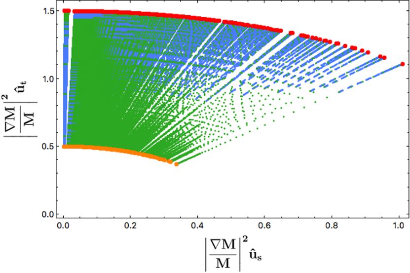
or a sublattice satisfying the WGC bound. When the gauge coupling goes to zero, all these
states become light since the mass has to decrease at a rate at least as fast as the charge.
The absence of free parameters in quantum gravity [3] implies that gauge couplings are
parametrized by the vacuum expectation value of scalar fields, which necessitates that the
point of vanishing gauge coupling is at infinite distance in field space. This is necessary to
avoid restoring a global symmetry at finite distance, which should not occur in a consistent
theory of quantum gravity [9–12].
     It is tantalizing that both the WGC and the SDC predict the existence of light states
at weak coupling points. This suggests that they might be two faces of the same underlying
quantum gravity criterion, as observed in [13–16]. It is the aim of this paper to continue

                                                                                                   JHEP01(2021)176
this line of thought by making the connection as precise as possible in the context of Calabi-
Yau compactifications of Type IIB string theory. Whether there exists a gauge coupling
that goes to zero for every infinite field distance point requires further study, but we will
argue in favor of this possibility as long as the gauge coupling can correspond to a p-form
gauge field (as opposed to specifically a 1-form).
     If the same tower of states satisfies both the WGC and the SDC, it is possible to
formulate a single, precise statement that is satisfied in the limit of weak coupling. The
unification of these conjectures beautifully resolves the previously ambiguous aspects of
each statement. On the one hand, the main open question regarding the SDC concerns the
rate of decay of the characteristic mass scale of the tower; this rate appears as an unspecified
order one parameter in the conjecture. Fixing this order one number for a given theory is
essential in determining the precise phenomenological implications of the conjecture in the
context of cosmology or particle physics. However, if this same tower of states also satisfies
the WGC, then we can bound this factor in terms of the extremality bound for black
holes in that theory. The WGC, on the other hand, suffers less ambiguities in the form
of unspecified order one parameters: when it concerns particles and large black holes, all
numerical factors are in principle specified. However, it does not state how many and which
states should be light at small gauge coupling. Seen from this angle, the SDC suggests that
infinitely many WGC-satisfying states become light, motivating the identification of the
SDC as a Tower WGC in the weak coupling limits. It should be stressed that at no point in
this work do we use any of the Swampland conjectures to make statements. Rather, we are
focused on analyzing the effective theories resulting from Calabi-Yau compactifications to
inform the conjectures and eliminate O(1) factors. Whether the exponential factor of the
SDC can be fully determined by the extremality bound for black holes in the asymptotic
limits depends on whether the WGC in the presence of scalar fields is equivalent to a
repulsive force condition (i.e. the statement that there must exist a particle for which the
Coulomb force is stronger than the attractive gravitational force plus scalar interactions).
The latter condition was proposed in [13] as the proper generalization of the WGC in
the presence of massless scalar fields, denoted in [16] as part of the Scalar WGC, and
further relabeled in [17] as the Repuslive Force Conjecture (RFC). We will keep the latter
name in this paper to avoid confusion with the actual Scalar WGC [13] which simply
requires that the scalar force acts stronger than the gravitational force on the particle.
Whenever the extremality bound and the RFC coincide, the exponential factor of the SDC

                                             –2–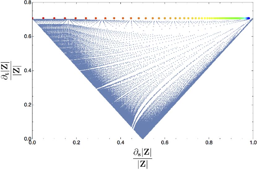
can be determined in terms of the scalar contribution to the extremality bound, which for
the case of a single scalar field can be directly inferred from the gauge kinetic function
as studied in [16]. That the extremality bound and force-cancellation condition coincide
was proposed [16] to occur in the limit of weak gauge coupling. We will extend this to
asymptotic limits in higher dimensional moduli spaces in which an arbitrary number of
scalar fields are taken to the large field limit, and show that the exponential factor of the
SDC can be bounded from above and below by the scalar dependence of the gauge kinetic
function, which is related to the extremality bound.
     In order to make all these relations precise and check them explicitly in controlled com-
pactifications of string theory, we are going to restrict ourselves to N = 2 supersymmetric

                                                                                                  JHEP01(2021)176
theories that arise from compactifying string theory on a Calabi-Yau threefold, following
the work initiated in [14, 18–20] (see [15, 16, 21–27] for other works identifying the towers
of states becoming light at the asymptotic limits of Calabi-Yau compactifications). Once
the conjectures are well understood and proven in supersymmetric setups with N ≥ 2,
less supersymmetric configurations, which are more useful for phenomenology, stand to be
explored (see [28–36] for attempts in this direction). However, it is important to note that
to talk about the SDC, one needs to be able to move in field space towards an infinite
distance singularity. This is one reason why N = 2 theories are interesting: they provide
a non-trivial setup with a moduli space. One might expect the conjecture to still hold
in field spaces with a scalar potential (regarded as one of the implications of the Refined
SDC [37]) as long as there is a mass hierarchy privileging particular trajectories such that
the conjecture can be applied to the bottom of the scalar potential. In that case, though,
the realization of the conjecture gets conflated with which types of potentials are allowed
in string theory, implying constraints on the latter (see [38] for an analysis initiating the
classification of flux potentials at the asymptotic limits).
     In [14] (see also [18–20]), a tower of states in these N = 2 theories with the correct
properties to satisfy the SDC was identified as a monodromy orbit of BPS states becoming
light at the infinite field distance limits of the moduli space of vector multiplets. From
a microscopic point of view, BPS states correspond to D3-branes wrapped on special La-
grangian 3-cycles that arise as particles in the 4d theory and can become massless at the
singularities of the complex structure moduli space of Type IIB on a Calabi-Yau threefold.
These states are charged under the 4d U(1) gauge fields that arise from dimensional re-
duction of the Ramond-Ramond 4-form C4 , and are thus perfect candidates to also satisfy
the WGC. We will explicitly calculate the charge-to-mass ratio of these BPS states in the
4d theory and compare with the black hole extremality bound specific to the theory in
the infinite distance limit. In doing so, we will show that indeed the same set of BPS
states satisfy the WGC, the RFC, and the SDC, and we will be able to place a bound
on the mass decay rate of the SDC in terms of the type of infinite distance singularity
that is being approached. These precise numerical bounds are valid for multi-moduli large
field limits of any Calabi-Yau and will be computed using the mathematical machinery
of asymptotic Hodge theory, which allows us to determine the leading dependence of the
gauge kinetic function on the scalar fields as a large field limit is approached. Notice that
the generalization from one field to multiple fields is in general highly non-trivial, and this

                                            –3–
is where loopholes to the WGC usually arise. It is only thanks to the powerful theorems of
asymptotic Hodge theory that we can overcome path dependent issues and give universal
bounds that cannot be tricked by any type of alignment mechanism. We would also like to
remark that asymptotic Hodge theory does not only provide useful tools, but we believe it
in important piece in the quest of abstractly identifying the mathematical structure distin-
guishing the swampland and the landscape. As postulated in [14, 18] and recently nicely
formulated in [27], the difference between generic 4d N = 2 supergravity effective theories
(special Kähler geometries) and N = 2 theories which can be completed to a consistent
theory of quantum gravity, lies precisely in the structures provided by Hodge theory.

                                                                                                   JHEP01(2021)176
     It should also be noted that regardless of the implications of the Swampland conjectures
for the space of possible low-energy effective theories, they can often teach us where to look
for interesting structures in string theory as a whole, as already happened in [14, 15, 18, 23].
We will see another example of this here as we analyze the charge-to-mass ratios of states in
our theory. The charge-to-mass ratio of BPS states turns out to form a degenerate ellipse
with only two non-zero principal radii, regardless of the number of scalar fields. These
principal radii can be determined in terms of the scalar dependence of the gauge kinetic
function when written in a basis adapted to the asymptotic splitting of the charge lattice,
which is guaranteed by Hodge theory. This enormously simplifies the task of determining
the extremality bound in these theories, as all BPS states with electric charges become
extremal in the asymptotic limits of the moduli space. Furthermore, in certain examples
we study how the degenerate directions are truncated by the BPS charge restrictions, and
the ellipsoid is capped off by the extremality surface associated to non-BPS black holes. It
seems that at least in these examples, the set of BPS states is enough to satisfy the WGC
convex hull condition [39], even taking into account directions in field space which do not
support BPS charges.

     The overall goal of this work is two-fold: first, to understand the structure of BPS states
in the asymptotic regimes of moduli space, and second, to use this knowledge to put a bound
on the mass decay rate of the states that become light according to the SDC. The outline of
the paper is as follows. In section 2, we will review how the notions of extremality and force-
cancellation change in the presence of massless scalars as well as review all the Swampland
conjectures that we aim to test in this work. In section 3, we will compute the charge-
to-mass spectrum of BPS states in a general setting, as well as give concrete examples
of this structure in compactifications with one and two moduli. In section 4, we will
describe how to compute the gauge kinetic function in terms of the type of infinite distance
singularity and thus read off the extremality bounds of electric black holes in general for
any asymptotic limit. With this information, we will be able to formulate general bounds
on the mass decay rate of the Distance Conjecture. In section 5, we provide some insight
into how such a framework may manifest in more general settings; for example, considering
non-BPS extremal solutions, and theories with N < 2. Finally, we conclude in section 6.

                                             –4–
2       Swampland conjectures in the presence of scalar fields

In this paper, we will test and sharpen the WGC and SDC by studying the properties
of BPS states and the interrelations that appear among them. In particular, we will
see how the WGC gets modified in the presence of scalar fields, yielding two possible
generalizations in terms of the black hole extremality bound or a repulsive force condition.
Both notions will coincide if the particles in question correspond to the asymptotic tower
of states predicted by the SDC, which further allows us to determine the exponential mass
decay rate in terms of the extremality bound.
     Consider a quantum field theory with abelian gauge fields and massless scalar fields

                                                                                                                      JHEP01(2021)176
weakly coupled to Einstein gravity, with action given by
                             Z       √
                                           R 1                   1

               S = MpD−2         dD x −h     − gij ∂µ φi ∂ µ φj − fIJ (φ)Fµν
                                                                          I
                                                                             F J,µν ,                        (2.1)
                                           2  2                  2

where gij is the field space metric and fIJ (φ) is the gauge kinetic function, which can
depend on the scalar fields.
     The WGC [4] states that in a quantum field theory with a weakly coupled gauge field
and Einstein gravity, there must exist a particle whose charge-to-mass ratio is larger than
the one associated to an extremal black hole in that theory, i.e. the theory must contain a
superextremal particle. In the absence of massless scalar fields, this implies that its charge
must be bigger than its mass in Planck units, so the WGC can also be formulated as the
statement that gravity acts weaker than the gauge force over this particle. Though these
statements are equivalent when there are only gauge forces and gravity, a crucial insight is
to realize that they can differ in the presence of massless scalar fields.
     Massless scalars alter the extremality bound of black hole solutions in a theory as
well as the no-force condition for particles. Therefore, there are two apparently different
generalizations of the weak gravity bound in the presence of scalars:

        • Weak Gravity Conjecture (WGC): there must exist a superextremal particle
          satisfying
                                   Q    Q

                                     ≥             ,                        (2.2)
                                   M    M extremal

                                                  Q
         where the extremality bound              M                  can depend on the scalar fields. Here
                                                          extremal
         Q2 = qI f IJ qJ with qI the quantized charges. This bound is what is commonly
         assumed to be the generalization of the WGC with scalar fields [17], as it preserves
         one of the original motivations that extremal black holes should be allowed to decay
         in a theory of quantum gravity. In the presence of several gauge fields, the WGC can
         be phrased as the condition that the convex hull of the charge-to-mass ratio of the
         states in the theory contains the extremal region1 [39].
    1
     The extremal region in the presence of scalar fields is not necessarily a unit ball; it needs to be determined
for each theory.

                                                          –5–
• Repulsive Force Conjecture (RFC): there must exist a particle which is self-
         repulsive, i.e. in which the gauge force acts stronger than gravity plus the scalar
         force,
                                     2
                                      Q       D − 3 g ij ∂i M ∂j M
                                           ≥         +                                 (2.3)
                                     M        D−2          M2
         where D is the space-time dimension and i, j run over the canonically normalized
         massless scalar fields. This bound was first proposed in [13] as the proper generaliza-
         tion of the WGC in the presence of scalar fields and renamed in [17] as the Repulsive
         Force Conjecture. Notice that saturation of this bound corresponds to cancellation of

                                                                                                                JHEP01(2021)176
         forces, where the scalar Yukawa force arises simply because the particle mass M (φ)
         is parametrized by a massless scalar.2 The argument for this bound stems from the
         expectation that black hole decay products should not be able to form gravitationally
         bound states.

     In a supersymmetric theory, BPS particles satisfy a no-force condition and will in-
deed saturate (2.3). Therefore, the RFC can be understood as an anti-BPS bound along
the directions of the charge lattice that can support BPS states. This is what led [40]
to formulate a sharpening of the WGC for which only BPS states in a supersymmetric
theory can saturate the WGC, yielding the striking result that any non-supersymmetric
AdS vacua supported by fluxes must be unstable [40, 41]. However, this conclusion re-
lies on this latter interpretation of the WGC as an anti-BPS bound and its fate becomes
unclear whenever (2.2) and (2.3) do not coincide, or whenever it is possible to have ex-
tremal non-BPS states still satisfying a no-force condition as occurs if there is some fake
supersymmetry [13, 42]. We will discuss more about this latter possibility in section 5.
     These two bounds (2.2) and (2.3) are in principle numerically different in the presence
of scalars, as emphasized in [17]. However, as we will see, they actually coincide in the
asymptotic regimes of moduli space,3 congruent with the proposal in [16] that they should
coincide in the weak coupling limits. In [16], both bounds were shown to match explicitly for
the weak coupling limits in 6D F-theory Calabi-Yau compactifications with 16 supercharges.
In this paper, we will show that both bounds indeed coincide at any infinite field distance
limit of the complex structure moduli space of four dimensional IIB Calabi-Yau string
compactifications, i.e. for N = 2 four dimensional effective theories with 8 supercharges.
Further connections between the WGC and the RFC can be found in [17, 49–52].4
     In the infinite field distance limits, there is another Swampland conjecture which also
predicts the presence of new particles becoming light:
   2
    When the mass of a particle χ is parametrized by a massless scalar field φ, there is a Yukawa force
interaction arising from
                                L ⊃ M 2 (φ) χ2 = 2M (∂φ M ) φ χ2 + . . .                          (2.4)
as emphasized in [13], where ∂φ M plays the role of the scalar charge.
   3
     This coincidence might also be used to fix the order one factor in the WGC applied to axions [4, 43–48],
since the notion of extremality is not well defined in the case of instantons.
   4
     In particular, it is proved that extremal black holes (but not particles) always have vanishing self-
force [50], that particles which are self-repulsive everywhere in moduli space are superextremal [51], and
that those that have zero self-force everywhere, and nowhere vanishing mass are extremal [51].

                                                   –6–
• Swampland Distance Conjecture (SDC): when approaching an infinite distance
     point in field space, there must exist an infinite tower of states becoming exponentially
     light with characteristic mass

                               M ∼ M0 exp (−λ∆φ) as ∆φ → ∞,                                                   (2.5)

     where ∆φ is the geodesic field distance. Here λ is an unspecified parameter which is
     conjectured to be λ ∼ O(1).

     As already noticed in [14, 16], whenever there is a gauge coupling that goes to zero
in the infinite field distance limit, it is possible to identify a tower of states becoming

                                                                                                                      JHEP01(2021)176
exponentially light according to the SDC that also satisfies the WGC. Hence, the SDC
suggests a stronger version of the WGC for which there must be not only a single particle
but a sublattice or a tower of particles satisfying the WGC bound. In the past years, a
lot of effort has been dedicated to rigorously identifying the tower of particles that become
light in the infinite field distance limits of Calabi-Yau string compactifications [14–16, 18–
27] (see also [13, 28–31, 53–58]). It is the aim of this paper to study the relation between
these conjectures in more detail, using the knowledge we have recently gained about these
towers to define the Swampland conjectures in a precise way. In particular, if the same
tower of particles satisfies both the SDC and the WGC, we can obtain information about
the unspecified parameter λ appearing in the SDC using the extremality bound of black
holes. More concretely, it is precisely the contribution from scalar fields to the extremality
bound that will determine mass scalar dependence of SDC tower, as we will explain below.
     At the moment, it seems that we have three different Swampland conjectures predicting
the existence of new light particles at weak coupling limits. Given the evidence from
string compactifications, this seems redundant, as they all refer to the same asymptotic
towers of particles. Hence, we would like to unify the above conjectures into a single
statement that seems to hold at every infinite field distance limit of the moduli space of
string compactifications. The statement goes as follows:

   • In any infinite field distance limit with a vanishing gauge coupling, there exists an in-
                                                            2              2
                                                         Q                Q
     finite tower of charged states satisfying           M        ≥       M                   where the extremality
                                                                                   extremal
     bound coincides with the no-force condition:
                                     2
                                 Q                       D − 3 g ij ∂i M ∂j M

                                                     =        +                                               (2.6)
                                 M        extremal       D−2         M2
     and the gauge coupling decreases exponentially in terms of the geodesic field distance.

    Note that this statement is stronger than the mild version of the WGC as it requires
the existence of an infinite tower and not just a single particle. It matches, however, with
stronger versions known as the sublattice or Tower WGC [5–8]. It also nicely fits with the
notion that the WGC is a quantum gravity obstruction to restoring a U(1) global symme-
try when g → 0, as the infinite tower of states implies a reduction of the quantum gravity
cutoff. It also reproduces the SDC, as the fact that the gauge coupling decreases expo-
nentially implies that the tower also becomes exponentially light in terms of the geodesic

                                                 –7–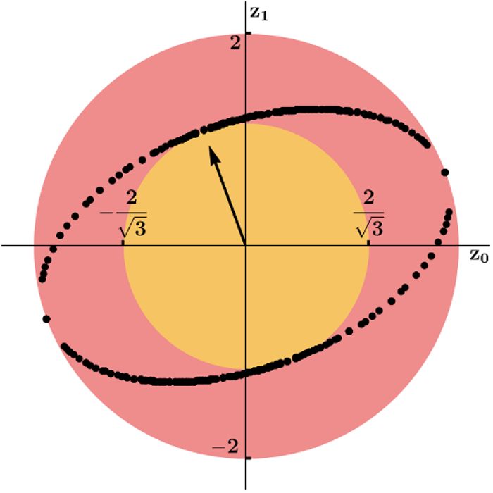
field distance. In addition, it further specifies the exponential rate of the tower, since it
is determined by the extremality bound. Hence, there remains no unspecified order one
parameter as in the original SDC.
     The scalar fields entering in (2.6) are those parametrizing the gauge kinetic function
of the gauge theory. If these scalars are massless, the extremal black hole solution involves
a non-trivial profile for the scalars which modifies the charge-to-mass ratio of the extremal
dilatonic Reissner-Nordstrom black hole. This extremality factor can be written as [59]
                                       2
                                   Q                   D−3 1 2

                                                   =      + |~
                                                             α| ,                          (2.7)
                                   M    extremal       D−2 4

                                                                                                   JHEP01(2021)176
where the second term is the scalar (dilatonic) contribution. In the particular case in which
the gauge coupling for all the gauge fields have the same dependence on the scalar fields,
|~
 α| becomes a numerical factor that can be easily read from the gauge kinetic function
                                        0 eαi φi in terms of the canonically normalized scalar
since the latter takes the form fIJ = fIJ
fields, where fIJ0 is a moduli-independent constant matrix. Otherwise, the extremality

bound becomes a more complicated function that depends non-trivially on the scalar fields
(see [60–62] for discussions of dilatonic black holes in more general settings).
     In principle, the second terms in (2.6) and (2.7) are numerically distinct if the WGC
and the RFC do not coincide, but, as already discussed, we will show that they coincide in
the regime approaching an infinite field distance point, so that

                                        α |2
                                       |~      g ij ∂i M ∂j M
                                             =                .                            (2.8)
                                         4           M2
The quantity on the right hand side is also known as the scalar charge-to-mass ratio and
plays a dominant role in the Scalar WGC proposed in [13] (see also [63–65]), for which
there must exist a state satisfying

                                       g ij ∂i M ∂j M   D−3
                                                2
                                                      >                                    (2.9)
                                             M          D−2
for any direction in field space. The appealing feature of this conjecture is that, if satisfied
by the SDC tower, it seems to imply that the exponential mass decay rate should be indeed
of order one. In fact, for a single scalar field, we can see that it relates to the exponential
factor λ of the SDC that appears in (2.5) as follows:

                                              1   ∂φ M
                                            λ= α=      .                                 (2.10)
                                              2    M
However, for more general setups with several gauge and scalar fields, the situation is
more complicated and the above identification (2.10) is not valid. First, when the gauge
kinetic function exhibits a different scalar dependence |~
                                                         α|, the scalar contribution to the
extremality bound cannot be directly read from the gauge kinetic function. Secondly, in
higher dimensional moduli spaces, path dependence issues come into play, invalidating
the identification of λ with the scalar charge-to-mass ratio. The exponential factor λ will
now be given by the projection of the scalar charge-to-mass ratio vector over the specific

                                                   –8–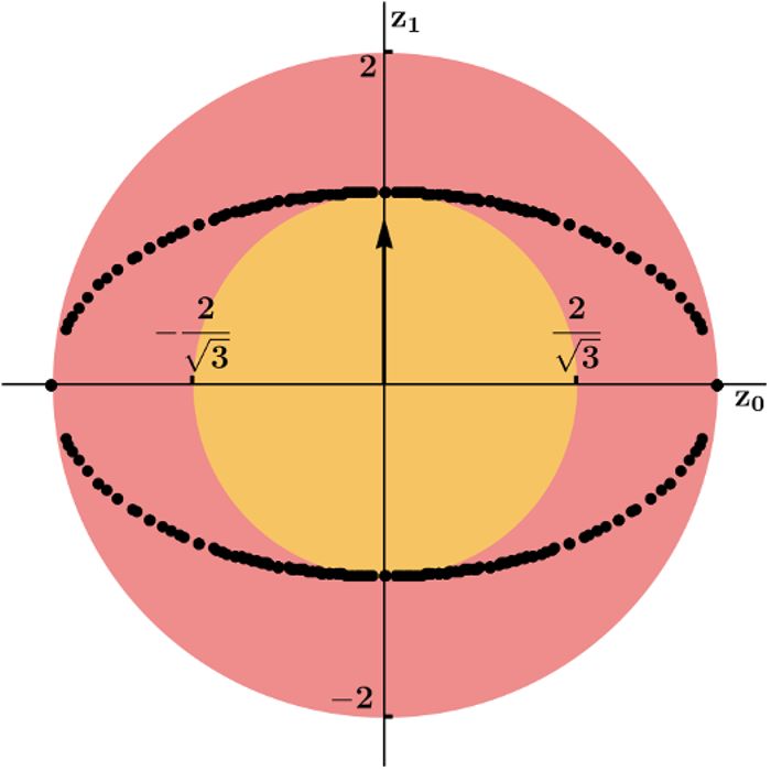
geodesic trajectory, as we will discuss in section 4.3, which can lower its value. Hence,
the extremality factor (or equivalently, the charge-to-mass ratio) will only give an upper
bound on the SDC exponential decay rate. Fortunately, we will still be able to place a
lower bound on the mass decay rate of the BPS tower using the scalar dependence of the
gauge kinetic function, but this lower bound will come from the individual αi associated to
the asymptotic splitting of charges that occurs at infinite field distance, as we will discuss
in section 4.3. In fact, these individual αi will still be associated to the scalar contribution
to the extremality bound of some particular black holes that satisfy (2.7).

     It is important to remark that the original SDC does not refer to any gauge coupling

                                                                                                                JHEP01(2021)176
going to zero at infinite field distance, so the tower of states is not necessarily charged.
Hence, the claim (2.6) only completely reproduces the SDC if there is a gauge coupling
going to zero at every infinite field distance limit. This is a stronger requirement than the
original SDC. Even though the limit g → 0 is known to always be at infinite field distance,
the opposite is not necessarily true. However, we believe that it is always possible to
identify some p-form gauge coupling vanishing at every infinite field distance of string
compactifications, which also relates to the proposal [14] in understanding the SDC as a
quantum gravity obstruction to restore a global symmetry.5 Furthermore, if the Emergent
String Proposal of [25] is true, every infinite field distance limit would correspond either to
a decompactification limit or a string perturbative limit, suggesting that it might always be
possible to identify at least a KK photon or a 2-form gauge field becoming weakly coupled,
supporting our statement. It has also been recently emphasized [66] that the SDC tower
always hints a weakly coupled dual field theory description, which goes in the same spirit.
We will comment more on this in section 5. Notice, also, that we are not requiring this
charged tower to be the leading tower, i.e. the one with the fastest decay mass rate. If it
is not, it can still be used to give a lower bound on the exponential mass decay rate of the
SDC, and therefore a precise upper bound on the scalar field range.

     Although some arguments can be made in general for the unification of all these con-
jectures in the asymptotic regime, in the context of N = 2 compactifications we can be
very precise. For this reason, we will focus on N = 2 four dimensional supergravity effec-
tive theories in the next two sections. We will calculate the charge-to-mass ratios of BPS
states and compare these results to the black hole extremality bounds. This will allow us
to compare the different possible generalizations of the WGC that we have reviewed in this
section, as well as make progress in sharpening the SDC. We will explicitly check (2.6) and
provide a bound on λ for every infinite field distance limit. In section 5, we will discuss
the realization of (2.6) in other setups beyond 4d N = 2 theories.

   5
    There are actually two types of global symmetries that are restored at the infinite field distance limits
of Calabi-Yau compactifications and that have been associated [14] to the SDC. One one hand, we have a
U(1) global symmetry coming from each gauge coupling that goes to zero. On the other hand, we have the
global continuous version of a discrete symmetry of infinite order (a monodromy transformation) which is
part of the duality group and that was used in [14] to populate the infinite tower of states.

                                                   –9–
3 BPS states and extremal black holes in 4d N = 2 effective field theories
In this section, we analyze the structure of BPS charge-to-mass ratios in the asymptotic
limits of the moduli space of 4d N = 2 theories. We will calculate the extremality bound
and show that the charge-to-mass ratio of BPS states lie on a degenerate ellipsoid with two
finite principal radii, regardless of the number of moduli. We will exemplify this in two
particular examples. In those examples, we will compare the BPS charge-to-mass ratios
with the extremal black hole bounds of those particular theories, as well as calculate the
lower bound on the mass decay rate |λ| of the SDC. In section 4, we will compute the
numerical value of these radii in terms of the type of asymptotic limit in full generality.
JHEP01(2021)176
3.1 Review: N = 2 EFTs and BPS states in Calabi-Yau compactifications
Consider a Calabi-Yau threefold characterized by a set of h2,1 complex structure moduli T i
which span a special Kähler submanifold. Compactifying type IIB theory on this Calabi-
Yau threefold results in a four-dimensional effective theory with N = 2 supersymmetry
and nV = h2,1 vector multiplets, yielding nV + 1 U(1) gauge fields of field strength Fµν I
with I = 0, . . . , h2,1 . The theory also contains hypermultiplets involving the Kähler moduli
deformations which we will ignore for the moment, since they are not relevant for our
purposes. The low energy bosonic effective action reads
R
Z
S= 4
d x − Kij̄ ∂µ T i ∂ µ T̄ j + IIJ Fµν
I
F J,µν + RIJ Fµν
I
(?F )J,µν , (3.1)
2
where Kij̄ , IIJ , and RIJ are determined by the geometrical data of the compactification.6
In particular,
Kij̄ = ∂i ∂j̄ K, IIJ = Im(NIJ ), RIJ = Re(NIJ ), (3.2)
where K is the Kähler potential
I
h i
K = −log i X FI − X I F I (3.3)
and
Im FIK Im FJL X K X L
NIJ = F̄IJ + 2i . (3.4)
Im FM N X M X N
Here {X I , F I } are the periods of the holomorphic (3, 0)−form of the Calabi-Yau threefold
and can be written as holomorphic functions of the scalars T i . They can be determined
in terms of a prepotential function F through FI = ∂X I F and FIJ = ∂I ∂J F . Note that
capital indices range from 0 to h2,1 , but that in the case where a prepotential exists we
can go to special coordinates where X I = (1, T i ) with i = 1, . . . , h2,1 . The complex scalars
have components
T i = θi + iti (3.5)
where θi are the axions and ti are usually dubbed as saxions.
6
Note that Kij̄ = 12 gij from the previous section.
– 10 –The theory also contains BPS particles that arise from D3-branes wrapped on special
Lagrangian 3-cycles whose volumes are parametrized by the complex structure moduli.
The mass of a BPS state is given by the central charge: M = |Z|, which can be written
Z = eK/2 (qI X I − pI FI ) (3.6)
and the normalized charge in (2.2) of this BPS state is given by Q2 = 12 |Q|2 [2], where |Q|2
is defined as
1
|Q|2 = − ~qT M~q, (3.7)
2
JHEP01(2021)176
pI
where ~q is the vector of integrally quantized charges: ~q = and
qI
I + RI −1 R −RI −1
M= (3.8)
−I −1 R I −1
Note that we can also write the normalized charge in terms of the central charge [67]:
|Q|2 = |Z|2 + K ij̄ Di ZDj̄ Z, (3.9)
where Di is the covariant derivative, which acts on Z as Di Z = ∂i Z + 12 Ki Z. The specific
form of the prepotential, and therefore the field and gauge kinetic metrics, depend on which
region of the complex structure moduli space of the Calabi-Yau threefold we are in. We
will see that in the asymptotic regimes of the moduli space, there is a well-defined notion
of electric and magnetic BPS states which become massless or infinitely heavy respectively
at the infinite field distance limit as long as we classify the trajectories in field space into
different growth sectors. Hence, a charge that is an electric BPS state which becomes
massless along one path may no longer become massless within a different growth sector.
By default, though, the reader can assume we are denoting the electric charges as qI unless
otherwise noted.
Note that not all possible combinations of quantized (electric and magnetic) charge
are actually associated to BPS states. The central charge (4.13) is only the mass that
a BPS state would have if the charges qI , pI are actually populated by a physical BPS
state. In characterizing the charge-to-mass ratios of these D3-branes, it will be necessary
to determine which choices of charge do correspond to BPS particles. In general, the
quantized charges that can support BPS states will exhibit a conal structure (analogous to
the effective cone of 4-cycles on the Kähler moduli side). The attractor mechanism [68–71]
tells us that in the presence of a BPS black hole, there is an effective potential for the
moduli in the theory, and that the dynamics of the scalars in this potential are such that
they all flow to a fixed point on the black hole horizon, regardless of the initial scalar profile
at spatial infinity. Thus, we learn that the BPS choices of quantized charges are those which
allow the scalars in the theory to flow to fixed points on the horizon of a black hole. Said
differently, if the “wrong” charges are picked for a black hole, the scalars in the theory
will not exhibit an attractor flow and the black hole is not BPS. The details of using the
– 11 –attractor mechanism to determine which states are BPS was analyzed in [72–76]. It is also
important to note that just because a given charge site is able to support a BPS state does
not mean that such a state exists in the theory. Therefore, when we refer to particular BPS
states, we are referring to charge lattice sites which can in principle be populated by a BPS
state. To determine if a given BPS state at a particular point in field space continues being
BPS when moving to a different point, one must study the presence of walls of marginal
stability [73, 77–84], as also done in [14] for the asymptotic limits. In this section, we will
ignore the possible presence of these walls and just discuss the conal strucuture of charges
that can in principle support BPS states, leaving a more detailed study to section 4.
JHEP01(2021)176
3.2 BPS and extremality bounds in the infinite distance limit
A primary goal of this work is to compare the BPS spectrum arising from general compact-
ifications of this type with the extremality bounds of black hole solutions in the resulting
4d effective theory. Having reviewed the key ingredients for calculating the charge-to-mass
ratios of BPS states in section 3.1, let us now begin to do this comparison. We will revisit
why BPS black holes are extremal in the asymptotic limits of the moduli space, implying
the identification of the above WGC and the RFC conjectures, and identify some partic-
ular solutions, which we will denote as single-charge states, that will play a crucial role
throughout the paper.
To analyze the extremality bound of black holes in the effective theory, we first note
that in the infinite distance limits of moduli space, the Kähler metric Kij̄ always behaves
to leading order as
di
Kiī = 2 + . . . (3.10)
4ti
where di is an integer associated to the type of singular limit as we will discuss inqdetail in
section 4.1. Therefore, in terms of the canonically normalized scalar fields φi = d2i log ti ,
~
the gauge kinetic function IIJ will generically have exponential dependence: IIJ ∼ eα~ ·φ .
Thus, the black hole solutions of this theory are Reissner-Nordstrom dilatonic black holes.
For black holes charged under a single gauge field with a dilatonic coupling, the extremal
charge-to-mass ratio is given by (2.7)7
r
Q 1 2
= 1 + |~
α| (3.11)
M extremal 2
where we have specialized to a black hole charged under a 1-form gauge field in 4 dimensions.
If the black hole is charged under several gauge fields with different scalar dependencies,
the dilatonic contribution to the extremality bound cannot be simply read from the gauge
kinetic function and will depend on the scalars themselves.
On the other hand, the “no-force” condition is given by the BPS bound in our N = 2
setup: s
Q ∂i |Z|∂j̄ |Z|
= 1 + 4K ij̄ . (3.12)
M BPS |Z|2
7
Note that we have switched notation to Q as defined in (3.7) which involves an extra factor of 2.
– 12 –Comparing the above two equations, we can see that in order to show equality of the
extremal bound and the BPS bound, it suffices to show that the gauge kinetic function
IIJ and the absolute value squared of the central charge |Z|2 have the same functional
~
dependence on the scalars, i.e. that |Z|2 ∼ eα~ ·φ .
In section 4.2, we will give a general proof of this correlation between the central charge
and the gauge kinetic function for any number of moduli and gauge fields in any asymptotic
limit by using the growth theorem of asymptotic Hodge theory. Here, however, we give some
preliminary insight into why this holds in the well-studied large complex structure limit.
In theories with N = 2 supersymmetry, the gauge kinetic function and the field metric
are related in the large complex structure limit as
JHEP01(2021)176
−1 6 1 0
IIJ =− , (3.13)
κ 0 1 K ij̄
4
where we have set the axions to zero for the moment. Here, κ is related to the Kähler
potential: κ = 34 e−K and the Kähler potential can be written in terms of the periods as
in (3.3). Thus, we can rewrite the gauge kinetic function as
I
−1 4Im(X FI )−1 0
IIJ = I
. (3.14)
0 Im(X FI )−1 K ij̄
On the other hand, the mass squared is
−2|q T ηΠ|2
|Z|2 = I
, (3.15)
Im(X FI )
0 −I
where we have introduced the symplectic matrix η = to denote the symplectic
I 0
product in the central charge (3.6). For electric states with charge qI , the symplectic
product selects the periods X I = 1, T i . If we now focus on states charged under a single
gauge field, such that either q0 6= 0 or q1 6= 0, we find
−1
III ∝ |ZI |2 , (3.16)
I
−2qI2 ΠI Π
where |ZI |2 = J with no sum in the numerator, since the product |q T ηΠ|2 is pro-
Im(X FJ )
portional to 1 for a single-charge state with q0 charge or to K iī for a single-charge state
with qi charge.
For the above argument it is very important that we have not turned on several charges
associated to a different behavior of the gauge kinetic function at the same time. This
notion of single-charge state will be extensively used throughout the paper, so let us explain
it a bit more. A single-charge state is a state which carries charge only under a single 8 gauge
8
Actually, it can be charged under several gauge fields as long as they all have the same scalar dependence
on the gauge kinetic function. See section 4.2 for a very precise definition of a single-charge state in terms
of the charge splitting associated to the asymptotic limit.
– 13 –field whose gauge kinetic function can be written to leading order as single exponential
~
IIJ ∼ eα~ ·φ in terms of the canonically normalized fields. In other words, it corresponds to
a black hole whose extremality bound is simply given by the above dilatonic extremality
formula (3.11), where α is a constant corresponding to the exponential rate of the gauge
kinetic function. Though this is a basis-dependent definition, it is a well defined notion
in the asymptotic limits of moduli space. This condition selects a very particular basis of
charges which will be introduced in section 4. At this stage, let us simply add that this
basis is associated to an asymptotic splitting of the charge space into nearly orthogonal
subspaces which is guaranteed by the sl(2)-orbit theorem of Hodge Theory that will be
discussed in more detail in section 4.1. As remarked in [14, 18, 27, 85], the structures
JHEP01(2021)176
provided by Hodge theory are key to distinguish what N = 2 supergravity theories can
actually arise from string theory, so we do not expect our results to be necessarily valid
for any supergravity theory but only those consistent with a quantum gravity embedding.
The existence of these single-charge states will allow us to determine the shape that the
charge-to-mass ratio of BPS states trace out in the next section. We will identify these
single-charge states in examples in sections 3.4 and 3.5 but leave their general identification
in any asymptotic limit to section 4.2, where we will also provide the numerical result for
their charge-to-mass ratios in terms of discrete data associated to the infinite field distance
limit. At the moment, let us just remark that the charge-to-mass ratio of these single-charge
states is simply given by a numerical factor (independent of the moduli) that can be read
from the gauge kinetic function or equivalently computed from the central charge since:
K ij̄ ∂i |Z|∂j̄ |Z|
α |2 = 8
|~ (3.17)
|Z|2
The fact that the moduli dependence of the gauge kinetic function and the mass
squared are identical implies that the extremality bound and the BPS bound are equal.
Let us also notice that the presence of axions will only shift the identification of single-
charge BPS states, as will become clear throughout the next sections, but it is always
possible to find a basis of charges such that the associated single-charge BPS states satisfy
the above property.
What about BPS states that are charged under more than one gauge field? If the gauge
fields have a different scalar dependence, the extremality formula (3.11) is no longer valid,
and one has to solve the full BPS flow equations of the attractor mechanism in order to find
a extremal solution. Notice that (3.11) is only a particular solution of these flow equations.
Any other solution of the BPS flow equations will correspond to a BPS extremal back hole
as well. These flow equations have been extensively studied in the literature for N = 2
setups where black holes exhibit a well-known attractor behaviour [68–71, 86–88], wherein
the scalars flow to fixed values on the horizon of the black hole, regardless of their initial
conditions at spatial infinity. This is known as the attractor mechanism. The fixed values
for the scalars at the horizon can be determined by minimizing the black hole potential
Vbh = Q2 . When this charge supports a BPS state so that (3.9) is satisfied, minimization
of the black hole potential is equivalent to finding a solution to ∂T i |Z| = 0 for the values
of the scalars on the horizon. We can see this by examining the form of the attractor flow
– 14 –equations. The most general spherically symmetric ansatz for a black hole solution is 4d
is given by
1
2 2U (r) 2 −2U (r) 2 2 2
ds = e dt − e dr + r dΩ2 . (3.18)
g(r)2
Assuming spherically symmetric moduli and electromagnetic fields, there is a reduced ef-
fective action [72]
Z ∞
1
b
S= dτ U̇ + gab Ṫ T˙ − c2 + e2U Vbh (T ) ,
2 a
(3.19)
2 0
JHEP01(2021)176
where r = c/ sinh cτ , g(r) = h(τ ) cosh cτ , and Vbh = |Q|2 as defined in (3.9). This describes
a system in which the scalars T i flow in the potential Vbh until a minimum is reached. This
flow is given by the BPS flow equations, which read:
U̇ = −eU |Z| (3.20)
i U ij̄
Ṫ = −2e g ∂j̄ |Z|. (3.21)
Notice that electric states have a mass and charge corresponding to a monotonically de-
creasing runaway function towards infinite field distance, so that there is no extremum of
the black hole potential at finite distance. This should be contrasted with the behavior of
dyonic black holes, whose charge and mass have minima at finite distance points in moduli
space. The fact that the electric black holes have this runaway behavior implies that the
scalar fields flow to φ → ∞ at the black hole horizon and the black hole entropy vanishes
since Z|φ→∞ = 0. This also occurs for the dilatonic black hole solutions in (3.11). That
the scalars flow to infinite distance at the horizon of the black hole means that the black
hole horizon is, in fact, singular; black holes carrying only electric charge naively have zero
size. The Weak Gravity Conjecture instructs us to compare the charge-to-mass ratios of
the electrically charged states in the theory to precisely these “small” black holes, so one
may wonder whether such an endeavor might run into trouble, given the runaway nature of
the attractor mechanism for these objects. Clearly, this singularity at the horizon does not
allow us to describe these small black holes within the supergravity approximation. How-
ever, the typical expectation is that stringy higher derivative corrections will eventually
correct the entropy to make it finite, although this is open for debate [89–93]. In any case,
small black holes can always be appropriately described in the full string theory brane or
worldsheet approach, in which case one obtains a non-vanishing value for the entropy [89].
In this paper, we will investigate the relation between the extremality bound of such black
holes and the charge-to-mass ratios of BPS states under the assumption that string theory
comes to the rescue to regularize these black hole solutions when approaching the hori-
zon. It should be noted, though, that in order to carry out our analysis, we don’t need to
know the value of the black hole entropy: the only information we need is the ADM mass
MADM = |Z| and the charge of the black hole Q, which are fixed by supersymmetry and
depend only on the values of the scalar fields at spatial infinity, and not on the dynamics
near the horizon. Therefore, even though the black holes of interest cannot be fully de-
scribed within the supergravity approximation, we are free to analyze the WGC and SDC
– 15 –in this context. Electric dilatonic black holes of this type have also been studied in [94–96]
in the context of the WGC and SDC. In [94] they were used as an example to argue for a
local version of the SDC, for which local excitations of an EFT cannot sample large field
excursions without inducing large curvature at a horizon or instabilities.
It should be noted that not all charges allow for a physical solution to the flow equa-
tions (3.20)–(3.21). For instance, it could happen that the central charge is driven to zero at
a regular point in field space. When this occurs, the attractor flow “breaks” before reaching
the horizon, providing a litmus test for determining which charges can, in principle, give
rise to BPS states [73]. However, imposing Z 6= 0 is not always enough to guarantee a BPS
JHEP01(2021)176
black hole solution, as there are other ways for the attractor flow to break down, which
must be taken into account to get the full set of charge restrictions. In section 3.5, we
will see an example in which we will fully determine what regions of the charge lattice do
not correspond to BPS directions. However, this does not mean that extremal black holes
do not exist in these regions. In section 5 we will demonstrate the existence of non-BPS
extremal black holes precisely in the quadrants of the charge lattice that do not support
BPS states, and show that they still satisfy a no-force condition, confirming unification of
WGC and RFC at the asymptotic/weak coupling limits.
Note that the matching between WGC and RFC tells us something very interesting
about the connection between the Swampland Distance Conjecture and black hole ex-
tremality bounds. Recall that the SDC tells us that at infinite distance, there should be an
infinite tower of states that becomes exponentially light, where the rate is an unspecified
parameter denoted as λ in (2.5). For the single-charge states satisfying (3.17), the rate is
now fixed in terms of the dilatonic contribution to the extremality bound
1 ~
M ∼ M0 e− 2 α~ ·φ (3.22)
where recall φi are the canonically normalized scalars and αi can be read from the gauge
kinetic function. The parameter λ associated to a geodesic will be a projection of α~ over
the geodesic trajectory, so it will be lower bounded by the individual αi ’s. For the rest
of this paper, and in particular in section 4.3, we will exploit this fact, along with our
knowledge of the asymptotic behavior of the gauge kinetic function, to put bounds on the
exponential factor λ appearing in the Swampland Distance Conjecture for any number of
scalar and gauge fields.
As already remarked, only for the particular set of single-charge BPS states does the
extremality factor reduce to a numerical factor that can be read from the gauge kinetic
function. In general, though, the charge-to-mass ratio of BPS states (and the extremality
bound) will depend on the moduli. So what is this value in general? Can it be bounded?
If so, we can use it to bound the exponential factor of the SDC. Determining the general
structure of BPS states and finding these bounds is the goal of the next section.
– 16 –3.3 General structure of BPS charge-to-mass spectra
We are interested in the structure of the charge-to-mass vectors of electrically charged BPS
D3-branes in Type IIB compactifications. By “charge-to-mass vector,” we mean the vector
|Q|
~z = Q̂ (3.23)
M
with Q defined in (3.7), which is the quantity of interest when checking the Weak Gravity
Conjecture in settings with multiple gauge fields [39]. We will show in this section that the
~z-vectors of BPS states lie on a degenerate ellipsoid. This ellipsoid has exactly two non-
JHEP01(2021)176
degenerate directions, regardless of the number of moduli, with principal radii determined
by the gauge kinetic matrix. This is one the most useful results of this paper.
To see this, recall that the mass of a BPS state is given by the central charge
|Z|2
=1 (3.24)
M2
Let us define the quantized “electric charge” ~qE (corresponding to states that become
~ E . Then the above
light in the infinite distance limit) and associated “electric periods” Π
expression can be written explicitly as:
T ηΠ
qE T η Π̄
qE
E E
I
=1 (3.25)
−2Im X FI M 2
where η is an anti-symmetric intersection matrix
0 −I
Z
ηIJ = γI ∧ γJ = (3.26)
X I 0
with γI an appropriate integral symplectic basis of 3-cycles on the Calabi-Yau, X.
We would like to write this expression in terms of the ~z-vectors. To do this, let’s define
a symmetric matrix G such that GT G = − 12 I. Then using ~z = M 1
G−1 ~q, we get
† T ~ ~ † η T G~zE
~zE G η ΠE Π E
−2
I
= 1. (3.27)
Im X FI
This can be written as a quadratic equation
T
~zE A~zE = 1 (3.28)
where A is a symmetric matrix
~ † ηT G
~ EΠ
GT η Re Π E
A = −2
I
(3.29)
Im X FI
Note what this implies about the structure of A: this is a block-diagonal matrix with two
sub-blocks, where each sub-matrix is given by the outer product of a vector with itself.
– 17 –This means that A has exactly 2 non-zero eigenvalues and h2,1 − 1 zero eigenvalues. The
non-zero eigenvalues are easily computed:
~†
Re Π ~E
η T Iη Re Π
E
γ1−2 =
I
, (3.30)
Im X FI
~†
Im Π ~E
η T Iη Im Π
E
γ2−2 =
I
. (3.31)
Im X FI
In summary, we have seen that the charge-to-mass vectors of BPS states lie on an ellipsoid
JHEP01(2021)176
with two non-degenerate radii given by the above eigenvalues. This is also consistent with
the fact that not all of these states are mutually BPS (otherwise they could fragmentate
to smaller BPS states when crossing a wall of marginal stability), so they are expected to
form an ellipsoid in the charge-to-mass ratio plane. However, note that pairs of states lying
along lines in the degenerate directions are mutually BPS. Let us calculate the eigenvalues
of the ellipsoid more explicitly. To do this, we first note that they are invariant under shifts
in the axionic variables θi (where T i = θi + iti ). This is because the periods transform
under axion shifts as:
†
~ E = e θ i Ni Π
Π ~ E,0 (3.32)
~ E,0 are the electric periods with all axions set to zero, and Ni is a nilpotent
where Π
monodromy matrix. This is called the Nilpotent Orbit Theorem [97] and is reviewed in
more detail in section 4.1. The gauge kinetic matrix transforms in a similar way,
iN † iN
I = eθ i I0 eθ i
, (3.33)
where I0 is the gauge kinetic matrix with the axions set to zero. Plugging these in to
eqs. (3.30) and (3.31), we see that the eigenvalues can be written as
~ † ) η I0 η T Re(Π
Re(Π ~ E,0 )
E,0
γ1−2 = I
(3.34)
Im(X FI )
~ † ) η I0 η T Im(Π
Im(Π ~ E,0 )
E,0
γ2−2 = I
(3.35)
Im(X FI )
These expressions are much easier to calculate explicitly, namely because when the axions
are zero, I0 is diagonal9 and the periods Π~ E,0 are either purely real or purely imaginary.
To give an explicit expression for the eigenvalues, let’s write them in terms of charge-to-
mass ratios of the single-charge states, as defined in the previous subsection. We will use
Q
the notation M to denote the charge-to-mass ratio of a single-charge state carrying
I
qE
I under the I th electric gauge field. This charge-to-mass ratio can be computed
charge qE
9
Actually, in general, the gauge kinetic matrix can be block diagonal in the infinite distance limit.
However, such a scenario corresponds to a higher-dimensional asymptotic subspace splitting, as explained
in section 4, and the results will not change.
– 18 –in terms of the electric periods and gauge kinetic function:
2 J
Q Im(X FJ )
= E,I
, (3.36)
M I E ΠE,I Π
I0,II
qE 0 0
with no sum over I. So we see that the eigenvalues of A can be written quite simply:
−2
Q
γ1−2
X
= (3.37)
M I
qE
i|Im(ΠE,I
0 )=0
−2
Q
γ2−2
X
= . (3.38)
JHEP01(2021)176
M I
qE
i|Im(ΠE,I
0 )6=0
This result is quite remarkable, since it means that we can completely determine the
structure of all BPS states in charge-to-mass ratio space just by computing the value of
the charge-to-mass ratio of the single-charge BPS states which, in the previous section, we
showed to be determined purely by the scalar dependence α ~ of the gauge kinetic function.
This might not seem well defined as it is basis-dependent, but the whole point is that there
is a special basis associated to each asymptotic limit in the moduli space for which the
above holds. This specific basis is associated to the sl(2) splitting which will be discussed
in section 4, implying that the eigenvalues γ1 , γ2 can be precisely calculated in terms of a
set of integers characterizing the infinite distance limits in Calabi-Yau threefolds.
The Weak Gravity Conjecture is satisfied if the convex hull of the charge-to-mass
vectors of the states of the theory contain the extremal black hole region. This extremal
region is sometimes simply identified with a unit ball, assuming that the extremality bound
is equal to 1 for every charge direction. In actuality, the extremal region need not be a
ball at all and can change from theory to theory. In 4d N = 2, since BPS black holes are
extremal in the asymptotic limits of the moduli space, this region will be equivalently given
by the value of the charge-to-mass ratio of BPS states along the directions supporting BPS
states. Hence, the ellipsoid with principal radii given by (3.37) and (3.38) corresponds to
the extremal region for electrically charged black holes.
As remarked in the previous section, not all regions in the charge lattice can support
BPS states. In general, we expect there to be inequalities governing the which directions
of the charge lattice are BPS directions of the form p(~q) > 0 with p a polynomial. Further-
more, our expectation is that these charge restrictions precisely coincide with truncating
the degenerate directions of the charge-to-mass ellipsoid. This expectation arises from the
fact that BPS states cannot become massless at non-singular points in moduli space [73],
and so charge directions with unbounded charge-to-mass ratios should be prohibited.
Let us also remark that even though it is clear that the WGC bound is satisfied
along BPS directions since BPS states themselves saturate the extremality bound, it is not
obvious at all whether BPS states are enough to satisfy the convex hull condition along any
direction in charge space. In section 5 we will compute the extremality bound for non-BPS
directions in a particular example, and show how the convex hull of BPS states contains
the entire extremal region, satisfying the WGC without the need of appealing to non-BPS
states.
– 19 –You can also read