Simplified Aberration Analysis Method of Holographic Waveguide Combiner - MDPI

Page created by Debra Caldwell
 
CONTINUE READING
Simplified Aberration Analysis Method of Holographic Waveguide Combiner - MDPI
hv
           photonics
Article
Simplified Aberration Analysis Method of
Holographic Waveguide Combiner
Wei-Chia Su 1 , Shao-Kui Zhou 1,2 , Bor-Shyh Lin 2 and Wen-Kai Lin 1,2, *
 1    Graduate Institute of Photonics, National Changhua University of Education, Changhua 50007, Taiwan;
      wcsu@cc.ncue.edu.tw (W.-C.S.); tommy848484.cop06g@nctu.edu.tw (S.-K.Z.)
 2    College of Photonics, National Chiao Tung University, Hsinchu 30010, Taiwan; borshyhlin@nctu.edu.tw
 *    Correspondence: alan0734.cop04g@nctu.edu.tw
                                                                                                    
 Received: 5 August 2020; Accepted: 9 September 2020; Published: 10 September 2020                  

 Abstract: Generally, the diffractive waveguide combiner and computer-generated hologram (CGH)
 technique have the potential to achieve compact head-mounted display (HMD) with a natural 3D
 display function. However, the diffractive waveguide combiner will degrade the image quality
 because of aberration. In order to resolve this issue, the complex analysis based on the ray-tracing
 method is necessary. Since the major aberration of the waveguide combiners is only astigmatism
 and anamorphic distortion, only these two aberrations were discussed in this paper. Furthermore,
 two common waveguide structures were discussed here. In total, four formulas were summarized
 to analyze aberration and anamorphic distortion in these two structures. Finally, the simplified
 formulas were verified with the commercial ray-tracing software Zemax. The calculated results of
 the proposed method match the simulation of Zemax software well. Therefore, the aberration of an
 arbitrary similar diffractive waveguide can be analyzed by the proposed method. This will make the
 designing process simpler and faster.

 Keywords: head-mounted display; computer-generated hologram; aberration analyzation;
 holographic waveguide

1. Introduction
     Display technology has been developing for decades. In recent years, the HMD devices have
received growing attention [1,2]. The HMDs are suitable to achieve the augmented reality (AR) function
due to their portability. Furthermore, the HMDs can provide autostereoscopic images without viewing
zone limit. However, the traditional stereoscopic imaging with two 2-D images is possibly causing the
vergence–accommodation conflicts [3]. In order to resolve this issue, providing 3D images with depth
information is necessary.
     The holography technique is an ideal method to project natural 3D images [4]. However, the
traditional holography technique records information optically and is difficult to achieve dynamic
display function. In contrast, the CGH technique computes the holograms numerically, and makes the
recording process become simpler [5–7]. Furthermore, the dynamic display function can be achieved by
displaying the holograms on a spatial light modulator (SLM). Then, the HMDs with 3D information can
be achieved utilizing the CGH techniques [8,9]. Since the general SLM can only modulate amplitude
or phase distribution, the phase information or the amplitude information of the hologram must be
eliminated. However, the elimination will degrade the image quality. In order to enhance the image
quality, the iterative algorithm [10,11] and the complex-amplitude modulation method [12–14] were
proposed successively.
     Excluding the image quality issue, the weight is also an important issue in similar devices. In order
to resolve this issue, the devices with waveguide combiner were also proposed [2]. In this method, the

Photonics 2020, 7, 71; doi:10.3390/photonics7030071                           www.mdpi.com/journal/photonics
Simplified Aberration Analysis Method of Holographic Waveguide Combiner - MDPI
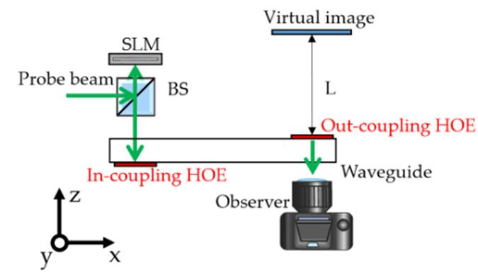
Photonics 2020, 7, 71                                                                                2 of 12

light is coupled into the waveguide and propagated inside the waveguide via total internal reflection
(TIR) on the waveguide surface. The in-coupler can be a diffraction element or a geometric structure
such as prism or wedge etc. Finally, the lights will be guided to the human eye by a diffraction
element. The diffraction element of in-coupler or out-coupler could be Raman–Nath grating [15,16]
or volume holographic element (VHOE) with Bragg grating [17–19]. The advantage of the former is
that achieving a wide viewing angle is easier. However, enhancing diffraction efficiency is difficult.
The VHOEs can achieve higher diffraction efficiency, but the rigorous angular selectivity will confine
the viewing angle. No matter the type, the diffraction waveguides cause the aberration and blur the
image. In order to correct the aberration, the aberration has to be analyzed in the waveguides with
symmetric [20,21] and asymmetric structures [22]. Concerning the latter, a geometric structure was
utilized as the in-coupler to reduce the power loss, and a VHOE was employed as the out-coupler. Both
the geometric structure and the diffraction element change the propagation angle of the light along a
single direction. It caused serious astigmatism and anamorphic distortion. On the contrary, the former
utilized two symmetric VHOEs as the in-coupler and the out-coupler. Since the angle changes caused
by two VHOEs are compensated to each other, the astigmatism becomes smaller, and the anamorphic
distortion is almost ignorable.
      In this paper, we propose a simplified method to analyze astigmatism and anamorphic distortion of
the symmetric and asymmetric structure. When the specification of the waveguides and the diffraction
angle of the normal incident ray on the HOE are known, astigmatism and anamorphic distortion can be
calculated easily. According to the literature, the waveguides caused aberration in only one direction.
The aberration for the different field perpendicular to this direction is almost constant. Considering
the viewing angle of the current SLM devices, the proposed method was simplified based on the
paraxial approximation. In the following sections, the symmetric and asymmetric structures similar
to [21,22] were utilized to verify the proposed method. If the diffractive efficiency is not considered, the
diffraction behavior of Raman–Nath grating and VHOE is the same. Therefore, the diffraction grating
formula was employed to replace H. Kogelnik’s coupled wave theory. It makes the proposed formulas
simpler. Furthermore, the formulas are also available for Raman–Nath grating—not only for VHOE.

2. Materials and Methods
      The schematic diagrams of the holographic waveguide element were shown in Figure 1. The
SLM provided object information, and the holographic waveguide combiners guide the information to
the human eye, then the observer can obtain virtual images. The symmetric structure as shown as
Figure 1a utilized two HOEs to couple optical information in and out the waveguide. The asymmetric
structure as shown as Figure 1b utilized a wedge with a polished surface as an in-coupling surface
and a HOE as an out-coupling element. The HOEs in these two structures are linear gratings in
which the grating vectors are parallel to the x-axis. Since the diopter of the HOEs and the wedge in
x-direction and y-direction is different, the waveguide element will cause astigmatism. Therefore,
the human eye obtains astigmatism virtual images when the SLM provides aberration-free objects.
On the other hand, the astigmatism objects will be obtained when the light of aberration-free images
incident the out-coupling HOE inversely. Then, the device can provide images without aberration
when the astigmatism objects are produced by the SLM.
      When the light of a virtual image was coupled into the waveguide at the Out-coupling HOE,
the field curvature curve of the object is shown in Figure 2. The distance from the out-coupling HOE
to the virtual image L is 250 mm. The diffraction angle for the normal incident light is 50 degrees.
The tilt angle of the wedge-shape in Figure 1b is 17.7 degrees. The field curvature curves as shown in
Figure 2 were simulated via the commercial ray-tracing software Zemax. The horizontal and vertical
axis marks the viewing angle and the distance respect to the last surface of combiners, separately. The
red curve shows the position of the imaging points in the y-z plane (Tangential plane), and the black
one shows that in the x-z plane (Sagittal plane). The distance of black lines became shorter because of
Simplified Aberration Analysis Method of Holographic Waveguide Combiner - MDPI
1a utilized two HOEs to couple optical information in and out the waveguide. The asymmetric structure
as shown as Figure 1b utilized a wedge with a polished surface as an in-coupling surface and a HOE as
an out-coupling element. The HOEs in these two structures are linear gratings in which the grating
vectors are parallel to the x-axis. Since the diopter of the HOEs and the wedge in x-direction and y-
direction    is different,
Photonics 2020,  7, 71        the waveguide element will cause astigmatism. Therefore, the human eye obtains               3 of 12
astigmatism virtual images when the SLM provides aberration-free objects. On the other hand, the
Photonics 2020, 7,
astigmatism         x FOR PEER
                 objects          REVIEW
                            will be  obtained when the light of aberration-free images incident the out-coupling          3 of 11
the  holographic        waveguides.       The   red  lines  in  the two   structures   were   located
HOE inversely. Then, the device can provide images without aberration when the astigmatism objects      at the same    distance
      When
because
are         thethe
     produced        light
                       the of
                 holographic
                   by           a virtual
                             SLM.          imagechanged
                                   waveguide        was coupled      into thedistance
                                                              the effective    waveguidefor xatfan
                                                                                                theonly.
                                                                                                    Out-coupling HOE, the
field curvature
       Photonics 2020,curve
                       7, x FORofPEER
                                  the REVIEW
                                       object is shown in Figure 2. The distance from the out-coupling                 HOE
                                                                                                                     3 of 11 to
the virtual image L is 250 mm. The diffraction angle for the normal incident light is 50 degrees. The
tilt angle of When
                 the the   light of a virtual
                       wedge-shape            image was
                                          in Figure        coupled
                                                       1b is          into the waveguide
                                                               17.7 degrees.    The field at  the Out-coupling
                                                                                            curvature    curves HOE,    the in
                                                                                                                 as shown
       field curvature curve of the object is shown in Figure 2. The distance from the out-coupling HOE to
Figure 2 were simulated via the commercial ray-tracing software Zemax. The horizontal and vertical
       the virtual image L is 250 mm. The diffraction angle for the normal incident light is 50 degrees. The
axis marks the viewing angle and the distance respect to the last surface of combiners, separately.
       tilt angle of the wedge-shape in Figure 1b is 17.7 degrees. The field curvature curves as shown in
The red    curve
       Figure        shows
                 2 were        the position
                          simulated   via the of  the imaging
                                               commercial          points software
                                                              ray-tracing   in the y-z  planeThe
                                                                                     Zemax.     (Tangential
                                                                                                   horizontal plane),   and the
                                                                                                              and vertical
black axis
        one marks
               showsthe  that   in the   x-z plane    (Sagittal   plane).   The   distance  of  black  lines  became
                            viewing angle and the distance respect to the last surface of combiners, separately.        shorter
becauseTheofredthecurve
                     holographic
                           shows thewaveguides.
                                        position of theThe   red lines
                                                         imaging         in in
                                                                    points  thethe
                                                                                 two
                                                                                   y-zstructures   were located
                                                                                       plane (Tangential   plane), at
                                                                                                                   andthe
                                                                                                                        thesame
distance
       blackbecause     the holographic
                one shows      that in the x-zwaveguide      changed
                                                 plane (Sagittal         theThe
                                                                   plane).    effective
                                                                                 distancedistance
                                                                                           of blackfor x fan
                                                                                                    lines     only.shorter
                                                                                                           became
                                       (a)                                                (b)
               because of the holographic waveguides. The red lines in the two structures were located at the same
               distance
              Figure
              Figure    because
                     1. The     the holographic
                        The schematic
                            schematic diagrams waveguide
                                      diagrams  of          changedwaveguide
                                                of the holographic  the effective
                                                                   waveguide      distance
                                                                               element:  (a)for
                                                                                        (a)     x fan only.
                                                                                             symmetric
                                                                                             symmetric   waveguide
                                                                                                         waveguide
                 400
              structure;
              structure; (b) asymmetric waveguide structure.
                         (b)                                                                                           400
                    350                                                         x-z plane                              350                                          x-z plane
                                     400                                        y-z plane                              400                                          y-z plane
                    300                                                           x-z plane                            300                                  x-z plane
                                     350                                                                               350
                                                                                                                (mm)
    Distance (mm)

                    250                                                           y-z plane                            250                                  y-z plane
                                     300                                                                     (mm)      300
                     Distance (mm)

                    200              250                                                                               200
                                                                                                                       250
                                                                                                       Distance

                    150              200                                                                               150
                                                                                                                       200
                                                                                                    Distance

                    100              150                                                                               150
                                                                                                                       100
                     50              100                                                                               100
                                                                                                                        50
                                      50                                                                                50
                       0                                                                                                 0
                        -3             0 -2        -1         0         1         2         3                            0-3    -2     -1           0       1         2         3
                                        -3    -2         -1         0       1         2         3                         -3   -2    -1         0       1       2         3
                                               x-field (degree)                                                                       x-field (degree)
                                                        x-field (degree)                                                             x-field (degree)
                                                        (a)                                                                                 (b)
                                                              (a)                                                                         (b)
              FigureFigure
                      2. The   fieldfield
                            2. The    curvature    plot
                                           curvature plotwhich
                                                           whichexported
                                                                  exported by
                                                                            by  commercialray-tracing
                                                                                            ray-tracing    software   shows
              Figure 2. The     field curvature    plot  which   exported    by commercial
                                                                                commercial ray-tracing software
                                                                                                           softwareshows
                                                                                                                      shows
              astigmatism   caused
                    astigmatism     by
                                 caused the
                                         by  waveguide
                                             the waveguideelements: (a)
                                                            elements: (a)symmetric
                                                                          symmetric waveguide
                                                                                    waveguide   structure;
                                                                                              structure; (b) (b) asymmetric
                                                                                                              asymmetric
              astigmatism caused by the waveguide elements: (a) symmetric waveguide structure; (b) asymmetric
              waveguide   structure.
                    waveguide   structure.
              waveguide    structure.

     The   The holographic
     The holographic
           holographic         waveguides
                          waveguides
                           waveguides        also
                                          also
                                            also  cause
                                                cause
                                                   cause anamorphic
                                                        anamorphic
                                                            anamorphic  distortion
                                                                        distortion    asasshown
                                                                             distortion     shown  in in
                                                                                              as shownFigure
                                                                                                           in 3,Figure
                                                                                                         Figure  which   were
                                                                                                                  3, which    were
                                                                                                                         3, which
      simulated
simulated    via   via Zemax.
                  Zemax.   In   In this
                               this gridgrid distortiondiagram,
                                          distortion      diagram, thethe ideal
                                                                          ideal  object
                                                                                  object   without
                                                                                             without aberration   is a is
                                                                                                         aberration     4 by
                                                                                                                          a 4 4by 4
were simulated via Zemax. In this grid distortion diagram, the ideal object without aberration is a
      grid as the solid grid. The crosses marked the real position of the grid intersection. In the asymmetric
grid
4 byas  the solid
      4 grid        grid.
               as the     Thegrid.
                       solid    crosses
                                      Themarked
                                           crossesthe    real position
                                                       marked     the realofposition
                                                                              the grid of  intersection.    In the asymmetric
                                                                                               the grid intersection.        In the
      structure, the object with serious anamorphic distortion was enlarged in the x-direction as shown in
structure,
asymmetric  the  object
               structure,with   serious
                            thethe
                                 object  anamorphic
                                         with in
                                               serious    distortion
                                                          anamorphic    was   enlarged
                                                                           distortion        in the  x-direction
                                                                                           was enlarged      in the as  shown
                                                                                                                      x-directionin
      Figure 3b.   However,        distortion     the symmetric     structure   is not serious     because the    symmetric
Figure
as shown3b.  However,
      linearingrating
                          the  distortion
                Figure compensated
                        3b. However,it.the  in the   symmetric
                                           In distortion
                                               this section, in the structure
                                                                the simplified   is  not
                                                                     symmetricformulas     serious
                                                                                     structure        because
                                                                                                   is proposed
                                                                                                 are  not seriousthe  symmetric
                                                                                                                  to because
                                                                                                                      predict the
linear  grating
symmetric          compensated
              linear  grating       it. In
                                 compensated
      astigmatism and anamorphic distortion.this   section,
                                                   it. In  thisthe  simplified
                                                                 section,   the     formulas
                                                                                 simplified        are   proposed
                                                                                                  formulas     are     to predict
                                                                                                                    proposed     to
astigmatism     and  anamorphic      distortion.
predict astigmatism and anamorphic distortion.

                                                                  (a)                                                                     (b)
                               Figure 3. The grid distortion diagram which exported by commercial ray-tracing software shows the
                                                 (a) caused by the waveguide elements: (a) symmetric waveguide
                               anamorphic distortion                                                      (b)      structure; (b)
                               asymmetric waveguide structure.
              Figure
              Figure 3.
                      3. The
                         The grid
                             grid distortion
                                  distortion diagram
                                             diagram which
                                                      which exported
                                                            exported by
                                                                     by commercial
                                                                        commercial ray-tracing
                                                                                    ray-tracing software
                                                                                                software shows
                                                                                                         shows the
                                                                                                                 the
              anamorphic
              anamorphic distortion
                            distortion caused
                                       caused by
                                               by the
                                                  the waveguide
                                                      waveguide elements:
                                                                 elements: (a)
                                                                            (a) symmetric
                                                                                symmetric waveguide
                                                                                          waveguide structure;
                                                                                                      structure; (b)
                                                                                                                  (b)
               2.1. Astigmatism Analysis
              asymmetric waveguide structure.
              asymmetric

2.1. Astigmatism Analysis
Simplified Aberration Analysis Method of Holographic Waveguide Combiner - MDPI
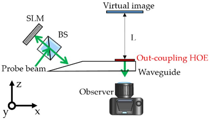
Photonics 2020, 7, 71                                                                                                       4 of 12

 Photonics 2020, 7, x FOR PEER REVIEW                                                                                        4 of 11
2.1. Astigmatism Analysis
        Figure 4 shows the schematic when the incident light of an arbitrary image point pass-through
       Figure 4 shows the schematic when the incident light of an arbitrary image point pass-through the
 the waveguides. The green line is the chief ray where the aperture stop is the human eye. The gray
waveguides. The green line is the chief ray where the aperture stop is the human eye. The gray line is
 line is an arbitrary off-axis ray, which deviates from the chief ray by a small angle                                 . Although
an arbitrary off-axis ray, which deviates from the chief ray by a small angle ∆φi . Although both the
 both the off-axis rays in x-fan and y-fan were considered in this section, only the ray in x-fan was
off-axis rays in x-fan and y-fan were considered in this section, only the ray in x-fan was drawn in this
 drawn in this figure. Here, we define                  , and               as the deviation angle of the off-axis rays in
                                                                       , angle
figure. Here, we define ∆φi,x and ∆φi,y as the              deviation              of the off-axis rays in x-fan and y-fan;
 x-fan   and  y-fan;  L is the distance   from    virtual   images    to   the  out-coupling
L is the distance from virtual images to the out-coupling HOE; Leye is the eye-relief;          HOE;         t isisthe
                                                                                                                    the thickness
                                                                                                                         eye-relief;
 t is  the thickness    of the waveguide;
of the waveguide; θi,x and θi,y are the incident   ,   and     ,
                                                             angleareof the chief ray at the out-coupling HOEthe
                                                                          the  incident   angle   of the  chief   ray   at       out-
                                                                                                                              in the
 coupling    HOE     in  the x-direction    and    y-direction;
x-direction and y-direction; θd,x and θd,y are the diffraction          ,   and angle   are  the  diffraction     angle
                                                                                     , in the x-direction and y-direction, in  the x-
 direction and
separately;   θob,xy-direction,
                    and θob,y areseparately;
                                   the angle of the   , and         , are
                                                          output light      inthe
                                                                               air angle
                                                                                   in the of the output
                                                                                           x-direction     light
                                                                                                         and       in air in the
                                                                                                              y-direction,      andx-
 direction   and   y-direction,   and
θt is the tilt angel of the wedge-shape in Figure 4b. Notice that the angle θob respects the normal line the
                                             is the  tilt  angel  of   the   wedge-shape       in Figure   4b.    Notice    that  of
 angle         respects   the normal   line  of  the  last  surface  of    the  waveguides.     The  symbols
the last surface of the waveguides. The symbols sx and s y are defined as the separation of the chief ray             and         are
 defined
and         as the separation
      the off-axis  rays at the of the
                                last    chief ray
                                      surface.    Theand   the off-axis
                                                        symbols    dx and   rays  at the
                                                                              d y are thelast surface.
                                                                                           distance      Thethe
                                                                                                      from    symbols
                                                                                                                  last surfaceand to
      are the
the focal   pointdistance
                   of x-fanfrom
                              and the   lastInsurface
                                   y-fan.       this case,to the  focal pointvaried
                                                              the aberration        of x-fanwithandthey-fan.  In this
                                                                                                        incident     anglecase,   the
                                                                                                                             in the
 aberrationnot
y-direction     varied   with the Therefore,
                   significantly.   incident angle       in the
                                                  only the       y-direction
                                                              image     points onnot the significantly.   Therefore,
                                                                                         x-axis (y = 0) were               only the
                                                                                                                   considered     in
 image    points
this section.     on  the  x-axis (y = 0)  were    considered     in  this   section.

                                      (a)                                                   (b)
       Figure4.4.The
      Figure      Theschematic
                      schematicdiagrams
                                diagrams ofof
                                            thethe
                                                 rayray  track
                                                      track    when
                                                            when thethe  information
                                                                     information      light
                                                                                  light     propagated
                                                                                        propagated     inversely:
                                                                                                   inversely: (a)
       (a) symmetric
      symmetric        waveguide
                  waveguide       structure;
                             structure;      (b) asymmetric
                                        (b) asymmetric          waveguide
                                                            waveguide       structure.
                                                                       structure.

2.1.1.
 2.1.1.Symmetric
        SymmetricStructure
                  Structure
     InInthe
          thesymmetric
              symmetricstructure,
                         structure,the
                                    thedistance
                                        distancefrom
                                                  fromthethelast
                                                             lastsurface
                                                                  surfacetotothe
                                                                              theobject
                                                                                  objectininthe
                                                                                             thex-z
                                                                                                 x-zplane
                                                                                                     plane(Sagittal
                                                                                                           (Sagittal
plane)  and  y-z plane (Tangential  plane)  of the points   on  the x-axis  can be described
 plane) and y-z plane (Tangential plane) of the points on the x-axis can be described as        as

                                                   = −sx cos θob,x ,
                                                                  
                                          
                                          
                                            d x =   ∆
                                                    ∆φob,x , 
                                                     −s                                                        (1)
                                           d y = =∆φ y cos θob,x ,
                                          
                                          
                                                               ∆ob,y ,

       Then,the
      Then,  theastigmatism
                 astigmatismcan
                             canbe
                                 bedefined
                                    definedasas
                                             ∆ =      −                                                                         (1)
                                            ∆d = dx − d y                                                                       (2)
       The relationship between     and     can be described as
      The relationship between θi and θd can be described as
                                                      ,                                                   ,
                            , =         −               =                        , ,   −
                                                  θ
                                                 ( i,x )                                   sin(θi,x )
                                                                                                    
                                      −1 λ − sin
                             θ                                   −1 sin θ
                           
                                = sin                    = sin                          −                                      (2)
                            d,x                                               d,x,0
                           
                           
                                        nΛ       n                                            n
                                                                            ,#                                                  (3)
                                                    =
                                                            "
                                                              sin ( θ     )
                                            θd,y, = sin−1
                           
                                                                     i,y
                           
                           
                           
                                                                  n

 where   is the period in the x-direction, is the wavelength, n is the refractive index of the waveguide
 and , , is the diffraction angle of the normal incident ray. Accordingly, when the incident angle is
 changed     , the variation of diffraction angle is
Photonics 2020, 7, 71                                                                                                          5 of 12

where Λ is the period in the x-direction, λ is the wavelength, n is the refractive index of the waveguide
and θd,x,0 is the diffraction angle of the normal incident ray. Accordingly, when the incident angle is
changed ∆φi , the variation of diffraction angle is
                                                 
                                                              cos(θi,x )
                                                  ∆φd,x = − ncos(θ ) ∆φi,x
                                                 
                                                 
                                                 
                                                                   d,x                                                           (4)
                                                      ∆φd,y = ∆φi,y /n
                                                 
                                                 
                                                 

      Then, the separation s in x-direction can be described as
                                                                                                                
            −L
                            !
                                  1       ( N + 1 ) t          1               t           ∆φob,x   1                 
 sx =              ∆φi,x             −           ∆φd,x           +                                     cos θob,x (5)
                                                                                                                 
                                                                                         
          cos(θi,x )         cos(θi,x ) cos θd,x
                                                                                                    
                                                           cos θd,x         cos θ0           n cos θ0             
                                                                                   ob,x                   ob,x

where N is the TIR times and θ0ob,x is the angle of output light θob,x in the waveguide considered Snell’s
law. The first term is the separation parallel to the x-axis at the out-coupling HOE. The second term is
the separation between two HOEs, and the third term is the separation from the in-coupling HOE to
the last surface. The final term behind the square bracket is utilized to obtain the component which is
perpendicular to the propagating direction. Since the angle of the incident ray and the output ray are
equal, Formula (5) becomes
                                                                                 
                                −L             (N + 1)tcos(θi,x )        t      
                         sx =  2             +                    +         cos(θi,x )∆φi,x                                (6)
                                                                                 
                                  cos (θi,x )
                                                             
                                                    ncos θd,x
                                                        3             ncos θi,x 
                                                                          2  0

where θ0i,x is the angle of incident ray considering Snell’s law. Similarly, the separation in the y-direction
can be described as
                                      −L∆φi,y −(N + 1)t∆φi,y           t∆φi,y
                                sy =             −                +                                         (7)
                                      cos(θi,x )
                                                                        
                                                    ncos θd,x        ncos θ0i,x

      Finally, when Formulas (6) and (7) are inducted into Formula (2), the aberration becomes
                                                                                                                     
                            ( N +  1 ) tcos3 (θ )     tcos2 (θ )               ( N +  1 ) tcos ( θ     )   tcos ( θ    )
                                                i,x           i,x                                   i,x             i,x
                                                                                                                  
             ∆d = L −
                                                                  
                                                    −          − L −                           −                       (8)
                                                                                                                      
                                                                                                               
                              n cos3 θd,x           ncos2 θ0i,x                n cos θd,x              ncos θ0i,x 

    Considering that the incident angle θi,x of the CGH systems is very small, Formula (8) can be
simplified as                                                       
                                       (N + 1)t           1      
                                ∆d =              1 −                                       (9)
                                                                      
                                                                
                                      n cos θd,x        cos θd,x 
                                                            2

     Here, the diffraction angle θd,x should be calculated according to Formula (3) for the arbitrary
incident angle θi,x .

2.1.2. Asymmetric Structure
    In the asymmetric structure with the wedge-shaped waveguide, the diffraction angle θd,x can be
computed following Formula (3), and the output angle θob can be computed according to Snell’s law.
The angle of the output ray θob can be described as
                                                             h              i
                                               θob,x = sin nsin    θt − θd,x
                                              
                                                          −1
                                                                h        i                                                    (10)
                                               θob,y = sin−1 nsin θd,y
                                              
                                              
Photonics 2020, 7, 71                                                                                       6 of 12

      Furthermore, when the incident angle θi is changed ∆φi , the change of the output ray is
                          
                                      n cos(θt −θd,x )        cos(θi,x ) cos(θt −θd,x )
                           ∆φob,x = − cos(θ ) ∆φd,x = cos(θ ) cos(θ ) ∆φi,x
                          
                          
                          
                                             ob,x                   d,x         ob,x                        (11)
                                                   ∆φob,y = ∆φi,y
                          
                          
                          

    According to the experience in the former paragraph, the separation in at the last surface can be
described as
                                                    cos(θi,x )∆φi,x cos(θd,x ) cos(θob,x )
                                                                  
                                   −L∆φi,x
                        
                         s x =                + D
                                  cos2 (θi,x )       n cos2 (θd,x )     cos(θt −θd,x )
                        
                                                                                                 (12)
                        
                                       s y = −L ∆φi,y + D              ∆φ
                        
                        
                                                                          i,y
                        
                        
                                               cos(θi,x )            n

where D is the distance from the out-coupling HOE to the wedge. For the x fan, the terms in the square
brackets are the separation parallel to the x-axis. The final term behind the square brackets is utilized to
obtain the component which is perpendicular to the propagating direction. Considering Formula (11)
and (12), the distance from the last surface to the object can be described as

                                     L cos2 (θd,x )   D cos (θob,x )
                                                               2
                                                                                           
                              d  =                  −                    cos  θ     − θ
                            
                               x
                            
                                      cos (θi,x        n cos (θt −θd,x )       ob,x     ob,x,0
                                             )
                            
                                        3                   2
                                                                                                             (13)
                                                               
                                                                                   
                                                            n cos θob,x − θob,x,0
                                                    L
                                                           −D
                            
                            
                                     dy =
                                               cos(θi,x )
                            

where θob,x,0 is the angle of the output chief ray when the x-field is 0. Additionally, the astigmatism
with paraxial approximation is
                                                                                     
                                   cos2 θd,x cos2 θob,x         D  cos2 θob,x           
                          ∆d = L                         − 1 −                 − 1              (14)
                                                                                            
                                                                          
                                    cos2 θ − θ                    n  cos2 θ − θ             
                                               t   d,x                        t    d,x

     Here, the output angle θob,x should be calculated according to Formulas (3) and (10) for arbitrary
incident angle θi,x .

2.2. Anamorphic Distortion
   Assuming the chief ray of an image point nearby the reference point probes the Out-coupling
HOE and the incident angle of the ray is

                                                    θi,x = θi,x + ∆θi,x
                                                (
                                                                                                             (15)
                                                        θi,y = ∆θi,y

where ∆θi,x and ∆θi,y are equal. The chief rays of this point and the reference point will converge at
the aperture stop. Since the position of the object can be predicted, the separation of these two rays at
the object plane can also be analyzed. Then, the anamorphic distortion can be predicted via the ratio of
the components of the separation in the x-direction and y-direction.

2.2.1. Symmetric Structure
      In the symmetric structure, the component in the x-direction considers paraxial approximation is
                                                                                                
                                     ( N + 1 ) t  1             ∆θi,x       ( N + 1 ) t   t  
              ∆X = Leye ∆θi,x + t +                     + t       + L −             − ∆θi,x    (16)
                                                                                                 
                                                                                   
                                      cos θd,x cos2 θd,x          n            ncos θd,x     n
Photonics 2020, 7, 71                                                                                       7 of 12

     The first term is the separation at the first surface. The second term is the total separation in
the waveguide. The third term is the product of the deviation angle ∆θi,x and the distance from the
waveguide to the object d y . Furthermore, the former formula can be simplified as
                                                           
                        t      (N + 1)t    1                 
                                                                              t
                                                                                       
             ∆X = Leye + + L +                        − 1∆θi,x = Leye + + L − ∆d ∆θi,x                (17)
                                                            
                                             
                         n      ncos θd,x  cos2 θd,x                      n

where ∆d is the result of Formula (9). Similarly, the separation in the y-direction can be described as
                                                                          
                         (N + 1)t        ∆θi,y       (N + 1)t     t 
                                                                                  
                                                                                         t
                                                                                             
   ∆Y = Leye ∆θi,y + t +           + t       + L −             − ∆θi,y = Leye + + L ∆θi,y          (18)
                                                 
                                                              
                          cos θd,x          n          n cos θd,x    n               n

      Then we define the effective distance from the human eye to virtual images as

                                                                       t
                                                    κ ≡ Leye +           +L                                  (19)
                                                                       n
      and the aspect ratio ξ of the anamorphic object can be defined as

                                                            ∆X   κ − ∆d
                                                    ξ≡         =                                             (20)
                                                            ∆Y      κ
When the image distance L is far enough, the aspect ratio must be equal to one.

2.2.2. Asymmetric Structure
      In the asymmetric structure, the separation in the x-direction can be described as
                                                                 
                                      t      D          cos θd,x cos(θo,x )  D
                                                                                    
                    ∆X = ∆θi,x Leye + +                                 + L−      ∆θob,x                 (21)
                                                         
                                                            
                                       n n cos2 θd,x  cos θt − θd,x             n

where ∆θob,x can be calculated as
                                                                     
                                                        cos θt − θd,x
                                          ∆θob,x   =                  ∆θi,x                              (22)
                                                     cos θd,x cos θob,x

     The first term is the separation at the wedge, and that term behind the square brackets is employed
to obtain the component which is perpendicular to the propagating direction. The second term is the
product of the deviation angle of output rays ∆θob,x and distance of object d y . Similarly, the separation
in the y-direction can be described as
                            
                                   t
                                           D∆θi,y    D
                                                                 
                                                                         t
                                                                             
                        ∆Y = Leye + ∆θi,y +       + L−     ∆θi,y = Leye + + L ∆θi,y                          (23)
                                   n          n        n                 n

      Finally, the aspect ratio can be described as
                                                                           
                                                                                ∆θi,x            ∆θ
                                                    t            D
                                           Leye +       +                       ∆θob,x   + L − Dn ∆θob,x
                                   ∆X               n       n cos2   (θd,x )                          i,x
                              ξ≡      =                                                                      (24)
                                   ∆Y                                       κ
      When the image distance L is far enough, the aspect ratio can be approximated as

                                                                ∆θob,x
                                                         ξ=                                                  (25)
                                                                ∆θi,x
Photonics 2020, 7, 71                                                                                                          8 of 12

3. Results
      In order to verify the proposed method, the calculated results of the formulas were compared to
the simulation results of Zemax in this section. Since the simulation in Zemax software was verified
so that results match the optical experiments in [21,22], the results of the proposed method should
match the results of Zemax. In this section, the thicknesses of the waveguide t in these two structures
were both 8 mm, and the refractive indexes were both 1.5195. The periods of three HOEs were equal
to each other. The diffraction angle of the normal incident ray was 50 degrees. The TIR times n in
the symmetric structure were 2. The tilt angle of the wedge-shape in the asymmetric structure was
17.7 degrees, and the distance from out-coupling HOE to the wedge D was about 45 mm. The field of
view (FOV) of the virtual images was ±2.4 degrees considering that the maximum diffraction angle
of the SLM with 6.4 um pixels was 2.38 degrees at 532 nm. When the image distance L was 250 mm,
 Photonics 2020, 7, x FOR PEER REVIEW                                                                    8 of 11
the astigmatism of the objects is shown in Figure 5. The horizontal axis is the viewing angle in the
x-direction.     Generally,
 shifted in Zemax.        Thethe image distance
                               maximum           L was
                                           deviation   much
                                                      was  2.04higher than the
                                                                 mm when        thickness
                                                                             x-field  was and  the eye-relief.
                                                                                           0°. However,     the
Therefore,    the   viewing  angle in the x-direction was approximated
 percentage error was smaller than 1.09% and was ignorable.              as the  incident angle θi,x . The red
plots in Figure 5a,b were calculated using Formulas (9) and (14), separately.

                -27                                                          -170
                               Zemax                                                         Zemax
                -30            formula (9)                                   -175            Formula (14)
                -33                                                          -180
    Δd (mm)

                                                                   Δd (mm)

                -36                                                          -185

                -39                                                          -190

                -42                                                          -195

                -45                                                          -200
                  -3      -2       -1         0   1   2      3                  -3      -2      -1         0   1    2          3
                                   x-field (degree)                                              x-field (degree)

                                        (a)                                                          (b)
        Figure5.
       Figure 5. The
                 The astigmatism
                      astigmatism with
                                  with different
                                       different x-field
                                                 x-field was
                                                         was predicted
                                                              predictedvia
                                                                       via Zemax
                                                                           Zemax software
                                                                                 softwareand
                                                                                           andthe
                                                                                               thesimplified
                                                                                                  simplified
        formulas: (a) symmetric waveguide   structure;  (b) asymmetric waveguide  structure.
       formulas: (a) symmetric waveguide structure; (b) asymmetric waveguide structure.

      In Figure
       When     the5a,image
                       the deviations
                             distance Lbetween   the results the
                                         was a variation,     of the proposed method
                                                                  astigmatism             and Zemax
                                                                                  of the central  field were   almost
                                                                                                         is shown   in
equal                                                                                        ◦
                                                                                     to −2.4as field.
 Figureto6.0,Inand   the maximum
                the symmetric         deviation
                                 structure,       was 0.17related
                                             astigmatism     mm corresponding
                                                                     to L was a constant,       shownIn inFigure
                                                                                                            Figure 5b,
                                                                                                                   6a.
the
 On results    of the the
     the contrary,      twoastigmatism
                            methods were     separated
                                        increased         byimage
                                                     as the  aboutdistance
                                                                     2 mm because
                                                                               L in thethe  Gaussianstructure.
                                                                                        asymmetric     image planeThe
slightly  shiftedalsoin Zemax.                                                                         ◦
 phenomenon              matches The   maximum
                                  the results       deviation
                                               in [22].         was
                                                        In Figure  6b,2.04
                                                                        the mm   when x-field
                                                                             deviations          was 0 . distances
                                                                                        with different     However,  L
the  percentage
 between            error
            different     was smaller
                         methods  were than   1.09%
                                        all about    and was
                                                   2 mm.       ignorable.
                                                           According     to these results, the simplified Formulas
      When
 (9) and  (14)the
                for image   distance
                     astigmatism      L waswere
                                   analysis    a variation,
                                                   verified.the astigmatism of the central field is shown in
Figure 6. In the symmetric structure, astigmatism related to L was a constant, as shown in Figure 6a.
On the contrary, the astigmatism increased as the image distance L in the asymmetric structure.
The phenomenon also matches the results in [22]. In Figure 6b,         0 the deviations with different      distances
         -33                             Zemax                                                     Zemax
L between different methods were all about 2 mm. According to these results, the simplified Formulas (9)
                                         Formula (9)               -300                            Formula (14)
and (14)-34for astigmatism analysis were verified.
                                                                             -600
                                                                 Δd (mm)
      Δd (mm)

                -35                                                          -900

                -36                                                        -1200

                                                                           -1500
                -37
                                                                           -1800
                      0    500          1000   1500   2000                          0    500         1000   1500        2000
                                        L (mm)                                                       L (mm)

                                        (a)                                                          (b)
        Figure 6. The astigmatism of the central field with different image distance was predicted via Zemax
        software and the simplified formulas: (a) symmetric waveguide structure; (b) asymmetric waveguide
        structure.
Figure 6. In the symmetric structure, astigmatism related to L was a constant, as shown in Figure 6a.
On the contrary, the astigmatism increased as the image distance L in the asymmetric structure. The
phenomenon also matches the results in [22]. In Figure 6b, the deviations with different distances L
between different methods were all about 2 mm. According to these results, the simplified Formulas
(9) and 2020,
Photonics (14) 7,
               for71astigmatism analysis were verified.                                        9 of 12

                                                                                     0                               Zemax
               -33                                 Zemax
                                                   Formula (9)                     -300                              Formula (14)
               -34
                                                                                   -600

                                                                        Δd (mm)
     Δd (mm)

               -35                                                                 -900

               -36                                                                -1200

                                                                                  -1500
               -37
                                                                                  -1800
                     0    500        1000   1500            2000                          0     500      1000   1500              2000
                                     L (mm)                                                              L (mm)

                                     (a)                                                                 (b)

      Figure 6. The
                  Theastigmatism
                       astigmatism of the central
                                      of the      fieldfield
                                             central     withwith
                                                               different imageimage
                                                                    different   distance  was predicted
                                                                                      distance           via Zemax
                                                                                                was predicted  via
      software
      Zemax     and the and
              software   simplified formulas:formulas:
                             the simplified    (a) symmetric    waveguidewaveguide
                                                           (a) symmetric     structure; (b) asymmetric
                                                                                         structure;      waveguide
                                                                                                    (b) asymmetric
      structure. structure.
      waveguide

      The aspect raio raio of
                            ofthe
                                theanamorphic
                                      anamorphicobjects
                                                     objectsin in   these
                                                                these  twotwo    structures
                                                                             structures    are are  shown
                                                                                                shown          in Figure
                                                                                                         in Figure    7. The7.
The  horizontal      axis  is the   viewing   angle  and    the   vertical  axis  is the  aspect   ratio
horizontal axis is the viewing angle and the vertical axis is the aspect ratio . The values simulated      ξ.   The  values
simulated
by Zemax wereby Zemax        werebased
                     calculated     calculated
                                          on thebased    on the grid
                                                  grid distortion        distortion
                                                                     diagram.          diagram.
                                                                                The solid   curvesThe      solid curves
                                                                                                      in Figure   7a,b werein
Figure   7a,bbywere
calculated              calculated
                   Formulas           by Formulas
                               (20) and               (20) and
                                          (24), separately.        (24), two
                                                              In these   separately.
                                                                              structures,In the
                                                                                             these  two structures,
                                                                                                  anamorphic             the
                                                                                                                  distortion
anamorphic       distortion
became significant,            became significant,
                          corresponding                corresponding
                                            to the reduction               to theand
                                                                 in the x-field,    reduction    in the x-field,
                                                                                        the deviation     increased and
                                                                                                                      as the
                                                                                                                          the
deviation
reduction increased
             in distance  as L.
                              theInreduction
                                     Figure 7a,in distance   L. In Figure
                                                  the anamorphic             7a, thewas
                                                                       distortion     anamorphic      distortion
                                                                                           not significant         was not
                                                                                                               because    the
Photonics 2020,
significant     7, x FORthe
             because     PEER   REVIEW linear grating compensated the aberration. When the distance L
                             symmetric                                                                                9 of
                                                                                                                         was11
symmetric     linear   grating   compensated the aberration. When the distance L was 250 mm, the aspect
250
ratiomm,   thecentral
       of the   aspect ratio
                         field of
                                wasthe1.13.
                                       central
                                            Thefield wasratio
                                                 aspect   1.13.grew
                                                                  The aspect
                                                                       closer ratio   grewthe
                                                                               to 1 with     closer  to 1 with
                                                                                                 farther         the farther
                                                                                                           distance   L. The
was highly significant as shown in Figure 7b. The aspect ratio grew closer to Formula (25) with the
distance
maximum    L. percentage
              The maximum         percentage
                              error             errorwas
                                     in this figure   in this  figure
                                                           0.17%.    Inwas
                                                                        the 0.17%.    In thestructure,
                                                                             asymmetric       asymmetric  thestructure,
                                                                                                               anamorphicthe
farther distance L. In this case, the aspect ratio of the central field in Formula (25) was 2.25.
anamorphic was highly significant as shown in Figure 7b. The aspect ratio grew closer to Formula (25)
Additionally, the ratio of the central field when L was 250 mm, 500 mm and infinity was 2.01, 2.12
with the farther distance L. In this case, the aspect ratio of the central field in Formula (25) was 2.25.
and 2.25, separately. The maximum percentage error in this figure was 0.32%.
Additionally, the ratio of the central field when L was 250 mm, 500 mm and infinity was 2.01, 2.12 and
2.25, separately. The maximum percentage error in this figure was 0.32%.

                                                   L=∝ Zemax
           1.25                                                                     2.8                                  L=∝ Zemax
                                                   L=∝ Formula (20)
                                                                                                                         L=∝ Formula (24)
                                                   L=500 Zemax
                                                                                                                         L=500 Zemax
           1.20                                    L=500 Formula (20)               2.6
                                                                                                                         L=500 Formula (24)
                                                   L=250 Zemax
                                                                                                                         L=250 Zemax
           1.15                                    L=250 Formula (20)               2.4                                  L=250 Formula (24)
                                                                              ξ
    ξ

           1.10                                                                     2.2

           1.05                                                                     2.0

           1.00                                                                     1.8
                 -3      -2     -1         0   1          2         3                     -3   -2     -1      0      1           2            3
                                x-field (degree)                                                      x-field (degree)

                                     (a)                                                                 (b)
      Figure 7.
      Figure 7. The
                  Theaspect ratio
                       aspect     of the
                               ratio     anamorphic
                                      of the          object
                                             anamorphic      with with
                                                           object different x-fieldx-field
                                                                        different    was predicted  via Zemax
                                                                                           was predicted  via
      software
      Zemax     and the and
             software   simplified formulas:formulas:
                            the simplified    (a) symmetric  waveguidewaveguide
                                                       (a) symmetric    structure; (b) asymmetric
                                                                                    structure;      waveguide
                                                                                               (b) asymmetric
      structure. structure.
      waveguide

4.
4. Discussion
   Discussion
    In
    In this
        thisstudy, thethe
              study,   equations of astigmatism
                          equations             and anamorphic
                                       of astigmatism           distortiondistortion
                                                       and anamorphic      of the diffractive
                                                                                      of the waveguide
                                                                                              diffractive
combiner
waveguide arecombiner
              presented for
                         are the CGH technique.
                              presented   for the Astigmatism of symmetric
                                                   CGH technique.            and asymmetric
                                                                    Astigmatism               structures
                                                                                     of symmetric    and
asymmetric structures can be calculated via Formula (8) and (13). The formulas were simplified as
Formulas (9) and (14) based on paraxial approximation. Furthermore, the anamorphic distortion of
these two structures can be calculated based on Formulas (20) and (24). Considering the commercial
SLM with a 6.4 um pixel size, the aberration was analyzed for ±2.4° FOV in this paper.
     Dismissing the limitation of SLMs, we compared the proposed method to the simulation of
Photonics 2020, 7, 71                                                                                                                                   10 of 12

can be calculated via Formula (8) and (13). The formulas were simplified as Formulas (9) and (14)
based on paraxial approximation. Furthermore, the anamorphic distortion of these two structures can
be calculated based on Formulas (20) and (24). Considering the commercial SLM with a 6.4 um pixel
size, the aberration was analyzed for ±2.4◦ FOV in this paper.
      Dismissing the limitation of SLMs, we compared the proposed method to the simulation of Zemax
with a larger field. In the simulation configuration employed in this paper, the maximum FOV of the
symmetric structure was from −10◦ to 9.4◦ , and in the asymmetric structure was from −5.2◦ to 9.4◦ .
The upper limit was limited by the TIR condition, and the lower limit was limited by the dimension
of the in-coupling surface. Smaller than the lower limit, the chief ray exceeded the boundary of the
in-coupling surface. The calculation results and the simulation results in this range when L was
250 mm are shown in Figure 8. In Figure 8a,b, the results of Formulas (8) and (13) match the results of
Zemax. The maximum deviation between Formulas (8) and (9) was 6.18 mm, and the percentage error
was 5.67% when the x-field was −10◦ . The maximum deviation between Formulas (13) and (14) was
6.92 mm, and the percentage error was 5.36% when the x-field was 9.4◦ . In Figure 8c,d, the maximum
percentage    error of the anamorphic analyzation based on Formula (20) was 2.53% when the x-field
 Photonics 2020, 7, x FOR PEER REVIEW
                                                                                                   was
                                                                                                 10 of 11
    ◦
−10 , and the maximum percentage error of Formula (24) was 2.23% when x-field was 9.4 .    ◦

                        0            Zemax                                               -120               Zemax
                                     Formula (8)                                                            Formula (13)
                       -20
                                     Formula (9)                                         -140               Formula (14)
                       -40
                                                                                         -160
            Δd (mm)

                                                                               Δd (mm)

                       -60
                                                                                         -180
                       -80
                                                                                         -200
                      -100

                      -120                                                               -220

                               -10       -5        0        5       10                           -6    -4     -2     0     2   4      6   8       10
                                           x-field (degree)                                                        x-field (degree)

                                                   (a)                                                                   (b)

              1.5                                               Zemax
                                                                                         3.5                                          Zemax
                                                                Formula (20)
                                                                                                                                      Formula (24)
              1.4
                                                                                         3.0
              1.3
                                                                                         2.5
                                                                               ξ
         ξ

              1.2
                                                                                         2.0
              1.1
                                                                                         1.5
              1.0
                                                                                                -6    -4     -2      0     2   4      6       8    10
                             -10        -5           0          5        10
                                                                                                                   x-field (degree)
                                         x-field (degree)
                                                   (c)                                                                   (d)
       Figure8.8. The aberration
      Figure           aberration analyzation
                                  analyzation for
                                               for large
                                                     largex-field:
                                                           x-field:(a)(a)astigmatism
                                                                           astigmatismof of symmetric
                                                                                          symmetric     structure;
                                                                                                     structure; (b)
      (b) astigmatism
       astigmatism   ofofasymmetric
                          asymmetricstructure;
                                      structure;(c)
                                                 (c) anamorphic
                                                      anamorphic ofof symmetric structure;
                                                                                    structure; (d)
                                                                                                (d)anamorphic
                                                                                                    anamorphicofof
      asymmetric
       asymmetricstructure.
                    structure.

     Considering the above information, we believe the proposed method is available for most
 5. Conclusions
diffractive waveguide HMDs, which is based on the current CGH technique. In fact, even
       In this paper, the aberration of two types of the holographic waveguide combiner are discussed.
whenemploying the SLM with the smallest pixel size (3.74 um for current commercial SLMs), the
 The major aberration caused by the holographic combiners is astigmatism and anamorphic distortion.
maximum FOV is about only ±4◦ . In the condition, the maximum deviation in Figure 8a was smaller
 In order to provide aberration-free images to the observer, producing an object with reverse
than 0.54 mm, and the maximum deviation in Figure 8b was smaller than 2.04 mm. Furthermore, the
 aberration is necessary. For each field, astigmatism is predicted via tracing the crossing point of the
percentage error of the anamorphic analyzation based on Formulas (20) and (24) was not larger than
 x-fan and the y-fan separately, and the anamorphic distortion is predicted via tracing the position at
0.64%.
 the object plane of the chief rays of the nearby points. In the proposed method, the astigmatism and
 the anamorphic distortion can be calculated easily when the specification of the waveguides and the
 diffraction angle of the HOE for the normal incident ray , , are known. Formulas (9) and (14) were
 utilized to predict the astigmatism of the object in the symmetric waveguide and the asymmetric
 waveguide, separately. Formulas (20) and (24) were utilized to predict the anamorphic distortion of
 the objects in the symmetric waveguide and asymmetric waveguide, separately. The results of the
Photonics 2020, 7, 71                                                                                       11 of 12

5. Conclusions
     In this paper, the aberration of two types of the holographic waveguide combiner are discussed.
The major aberration caused by the holographic combiners is astigmatism and anamorphic distortion.
In order to provide aberration-free images to the observer, producing an object with reverse aberration
is necessary. For each field, astigmatism is predicted via tracing the crossing point of the x-fan and the
y-fan separately, and the anamorphic distortion is predicted via tracing the position at the object plane
of the chief rays of the nearby points. In the proposed method, the astigmatism and the anamorphic
distortion can be calculated easily when the specification of the waveguides and the diffraction angle
of the HOE for the normal incident ray θd,x,0 are known. Formulas (9) and (14) were utilized to
predict the astigmatism of the object in the symmetric waveguide and the asymmetric waveguide,
separately. Formulas (20) and (24) were utilized to predict the anamorphic distortion of the objects in
the symmetric waveguide and asymmetric waveguide, separately. The results of the proposed method
are very close to the simulation of ray-tracing software Zemax, where the simulation of Zemax has
been proved for aberration correcting. Therefore, the aberration of an arbitrary device with a similar
holographic waveguide element can be corrected via the proposed method. It will make the designing
process simpler and faster.

Author Contributions: Writing—original draft preparation, W.-K.L.; writing—review and editing, W.-C.S. and
B.-S.L.; methodology, W.-K.L.; software, S.-K.Z.; funding acquisition, W.-C.S. supervision, W.-C.S. All authors
have read and agreed to the published version of the manuscript.
Funding: This work is supported by the Ministry of Science and Technology of Taiwan under contract MOST
108-2221-E-018 -018 -MY3.
Conflicts of Interest: The authors declare no conflict of interest.

References
1.    Shibata, T. Head mounted display. Displays 2002, 23, 57–64. [CrossRef]
2.    Li, H.; Zhang, X.; Shi, G.; Qu, H.; Wu, Y.; Zhang, J. Review and analysis of avionic helmet-mounted displays.
      Opt. Eng. 2013, 52, 110901. [CrossRef]
3.    Hoffman, D.M.; Girshick, A.R.; Akeley, K.; Banks, M.S. Vergence–accommodation conflicts hinder visual
      performance and cause visual fatigue. J. Vis. 2008, 8, 33. [CrossRef]
4.    Leith, E.N.; Upatnieks, J. Reconstructed wavefronts and communication theory. J. Opt. Soc. Am. 1962, 52,
      1123–1130. [CrossRef]
5.    Ogihara, Y.; Sakamoto, Y. Fast calculation method of a CGH for a patch model using a point-based method.
      Appl. Opt. 2015, 54, A76–A83. [CrossRef]
6.    Shimobaba, T.; Matsushima, K.; Kakue, T.; Masuda, N.; Ito, T. Scaled angular spectrum method. Opt. Lett.
      2012, 37, 4128–4130. [CrossRef]
7.    Matsushima, K. Computer-generated holograms for three-dimensional surface objects with shade and
      texture. Appl. Opt. 2005, 44, 4607–4614. [CrossRef]
8.    Moon, E.; Kim, M.; Roh, J.; Kim, H.; Hahn, J. Holographic head-mounted display with RGB light emitting
      diode light source. Opt. Express 2014, 22, 6526–6534. [CrossRef]
9.    Murakami, E.; Oguro, Y.; Sakamoto, Y. Study on Compact Head-Mounted Display System Using
      Electro-Holography for Augmented Reality. IEICE Trans. Electron. 2017, 100, 965–971. [CrossRef]
10.   Sypek, M.; Kolodziejczyk, A.; MikuĹ, G. Three-plane phase-only computer hologram generated with iterative
      Fresnel algorithm. Opt. Eng. 2005, 44, 125805–125807.
11.   Masuda, K.; Saita, Y.; Toritani, R.; Xia, P.; Nitta, K.; Matoba, O. Improvement of image quality of 3D display
      by using optimized binary phase modulation and intensity accumulation. J. Disp. Technol. 2016, 12, 472–477.
      [CrossRef]
12.   Gao, Q.; Liu, J.; Duan, X.; Zhao, T.; Li, X.; Liu, P. Compact see-through 3D head-mounted display based on
      wavefront modulation with holographic grating filter. Opt. Express 2017, 25, 8412–8424. [CrossRef]
13.   Mendoza-Yero, O.; Mínguez-Vega, G.; Lancis, J. Encoding complex fields by using a phase-only optical
      element. Opt. Lett. 2014, 39, 1740–1743. [CrossRef]
Photonics 2020, 7, 71                                                                                        12 of 12

14.   Li, X.; Liu, J.; Zhao, T.; Wang, Y. Color dynamic holographic display with wide viewing angle by improved
      complex amplitude modulation. Opt. Express 2018, 26, 2349–2358. [CrossRef]
15.   Eisen, L.; Meyklyar, M.; Golub, M.; Friesem, A.A.; Gurwich, I.; Weiss, V. Planar configuration for image
      projection. Appl. Opt. 2006, 45, 4005–4011. [CrossRef]
16.   Levola, T. Diffractive optics for virtual reality displays. J. Soc. Inf. Disp. 2006, 14, 467–475. [CrossRef]
17.   Piao, J.-A.; Li, G.; Piao, M.-L.; Kim, N. Full color holographic optical element fabrication for waveguide-type
      head mounted display using photopolymer. J. Opt. Soc. Korea 2013, 17, 242–248. [CrossRef]
18.   Han, J.; Liu, J.; Yao, X.; Wang, Y. Portable waveguide display system with a large field of view by integrating
      freeform elements and volume holograms. Opt. Express 2015, 23, 3534–3549. [CrossRef]
19.   Piao, M.-L.; Kim, N. Achieving high levels of color uniformity and optical efficiency for a wedge-shaped
      waveguide head-mounted display using a photopolymer. Appl. Opt. 2014, 53, 2180–2186. [CrossRef]
20.   Yeom, H.-J.; Kim, H.-J.; Kim, S.-B.; Zhang, H.; Li, B.; Ji, Y.-M.; Kim, S.-H.; Park, J.-H. 3D holographic head
      mounted display using holographic optical elements with astigmatism aberration compensation. Opt.
      Express 2015, 23, 32025–32034. [CrossRef]
21.   Lin, W.-K.; Matoba, O.; Lin, B.-S.; Su, W.-C. Astigmatism correction and quality optimization of
      computer-generated holograms for holographic waveguide displays. Opt. Express 2020, 28, 5519–5527.
      [CrossRef] [PubMed]
22.   Lin, W.-K.; Matoba, O.; Lin, B.-S.; Su, W.-C. Astigmatism and deformation correction for a holographic
      head-mounted display with a wedge-shaped holographic waveguide. Appl. Opt. 2018, 57, 7094–7101.
      [CrossRef]

                        © 2020 by the authors. Licensee MDPI, Basel, Switzerland. This article is an open access
                        article distributed under the terms and conditions of the Creative Commons Attribution
                        (CC BY) license (http://creativecommons.org/licenses/by/4.0/).
You can also read