Bends, Jogs, And Wiggles for Railroad Tracks and Vehicle Guide Ways
←
→
Page content transcription
If your browser does not render page correctly, please read the page content below
Bends, Jogs, And Wiggles for Railroad Tracks and Vehicle Guide Ways

                                    Louis T. Klauder Jr., PhD, PE.
                                              Work Soft
                                            833 Galer Dr.
                                     Newtown Square, PA 19073
                                           lklauder@wsof.com

                                        Preprint, June 24, 2002
                               Copyright © 2002 by Louis T Klauder Jr.
                                     International Patent Pending

ABSTRACT

In traditional design for railroad track other than “special work” the geometrical path of a track is
composed as a sequence of straight lines, circular arcs, and spirals. The present paper defines some
new geometrical shapes that can be incorporated into alignments for railroad tracks and other vehicle
guide ways. Where the new shapes are appropriate, alignments that incorporate them will give
dynamic performance superior to corresponding alignments whose only curved elements are spirals
and circular arcs.

The simplest of the new shapes are referred to as Bends, Jogs, and Wiggles. While these shapes have
been a part of every-day language for a long time, they do not appear to have been previously defined
for or used in geometrical design of tracks and guide ways.

The new shapes are defined within the framework of a recently developed method for design of
improved railroad track spirals. This paper reviews that method, notes situations in which the new
shapes can provide improved geometry, presents mathematical formulae by which the shapes can be
defined, and shows by examples how the shapes can be applied in some typical railroad track
situations. It is shown that the new shapes can be defined in terms of Gegenbauer polynomials and that
the known properties of those polynomials contribute both to understanding and application of the
shapes.

Among ways that the new shapes can be used to improve railroad track there are three that are
particularly encouraged. First, the Jog shape can be used to define turnout and crossover geometry that
is dynamically better than the geometry in current use. Second, when existing curves are being
re-aligned and their spirals are found to be too distorted for immediate restoration of ideal geometry,
the spirals can be modified by admixture of the new shapes and tamping with limited track throws can
then achieve smoothed alignments whose dynamic characteristics are relatively optimal. Third, when
existing curves are being upgraded for higher speeds and transition lengths need to be increased
without relocation of the curves, transitions based on combinations of spirals and Bends will be
dynamically better than corresponding compound transitions based on separate arcs and spirals.

The new shapes are applicable not only to railroad tracks but also to other vehicle guide ways
including, for example, maglev guide ways (magways), roller coaster tracks, and bobsled runs.

OUTLINE
1 Introduction
2 Review of Improved Spiral Design Method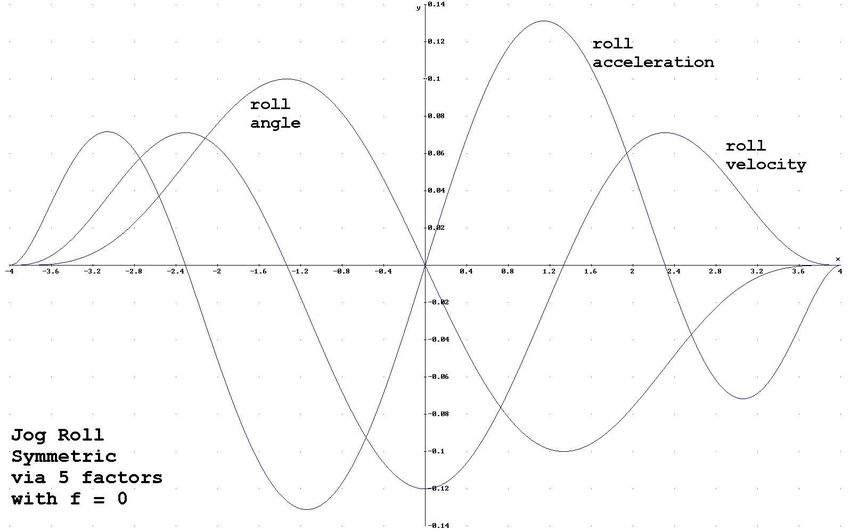
Bends, Jogs, And Wiggles for Railroad Tracks and Vehicle Guide Ways, Louis T Klauder Jr.            2
                                     (Preprint, June 24, 2002)

3    Constructing the roll acceleration for a Bend by overlapping two spirals
4    Constructing the roll acceleration for a Bend by inserting a factor
5    Constructing the roll acceleration for a Jog by overlapping three spirals
6    Constructing the roll acceleration for a Jog by inserting a factor
7    Jogs as shapes for turnouts and crossovers
8    Constructing the roll acceleration for a Wiggle by inserting a factor
9    Simplification and generalization by means of Gegenbauer polynomials
10   Using spiral, Bend, and Jog combinations to upgrade curves with inadequate offset
11   Classification of adjacent arc relationships
12   Modified Gegenbauer series for alignments that avoid obstacles
13   Modified Gegenbauer series for maintenance of track geometry
14   Conclusions
15   References.

1. Introduction

Recent publications (references 1, 2, & 3) have presented and demonstrated an improved way of
thinking about and calculating the geometry of transition spirals for railroad curves. Those publications
applied the improved method to the most common situation where a spiral makes a simple connection
between two adjacent segments of track with differing constant values of curvature.

The present paper explores the application of the improved method to more complex transition shapes
referred to as Bends, Jogs, and Wiggles.

Bends will be of value for track layout at locations where the track needs to change direction by a
“small” amount. The background is as follows. When an attempt is made to use the normal spiral –
curve – spiral sequence to accomplish a “small” turn, the spirals themselves accomplish the turn so that
the sequence changes to spiral – spiral. If the spirals employed are traditional linear spirals, then the
two spiral sequence has worse than usual dynamic characteristics where the two spirals meet. That
problem can be ameliorated by use of improved spirals. However, it will be more logical to employ a
shape designed for this situation. The Bend is designed to be such a shape. It is defined using a
conceptual framework first developed for improving the design of spirals and will give good dynamic
performance in “small turn” situations.

Jogs are defined below for situations where the track needs to curve quickly in one direction and then
quickly in the other direction and where the curvature of the track needs to keep changing throughout
both curves. Jogs can be used for the design of turnouts and crossovers. A Jog can also be used in
continuous track where a clearance obstruction on one side is followed fairly closely by an obstruction
on the other side.

A Wiggle bends to the right, then to the left, and then to the right, or vice-versa. A Wiggle can be used
where an obstacle on one side requires a local deviation by what would otherwise be a straight path.
Shapes like Wiggles but with more than three bends can also be defined.

This paper gives formulae for Bends, Jogs, and Wiggles and illustrates track shapes which can be
obtained from them. The author expects to be able in a future paper coauthored with others to present
results of simulations like those of reference 3 that will show how predicted vehicle dynamic responses
Bends, Jogs, And Wiggles for Railroad Tracks and Vehicle Guide Ways, Louis T Klauder Jr. 3
(Preprint, June 24, 2002)
to Bends, Jogs, and shapes defined by Gegenbauer polynomial series compare with predicted vehicle
responses to corresponding traditional geometries.
The new shapes are applicable to any guide ways on which vehicle speeds are high enough relative to
guide way curvatures so that centripetal accelerations are important. Other examples of guide ways in
that category are guide ways for maglev vehicles, roller coasters tracks, and bob-sled runs.
2. Review of Improved Spiral Design Method
The present paper is based on an improved method for designing track geometry shapes in which the
curvature varies with distance. This Section gives an overview of that method as applied to the design
of the spiral, which is the simplest such shape.
The main novelty of the improved method is that design is begun not by consideration of competing
shapes but rather by considering competing forms for the roll of the track as a function of distance. The
rationale for the improved design method is the proposition that the primary job of a shape element in
which curvature changes with distance is to cause a vehicle that traverses it to have its roll angle
change from one steady value to another with the least fluctuation of lateral force applied to the rails
and with the least fluctuation of lateral and roll accelerations applied to vehicles. This premise focuses
attention on the vehicle’s rotation about its roll axis as it traverses the spiral and on the character of the
roll and linear accelerations to which the vehicle is subjected in that process. For reasons explained in
references 1, 2, 3, 4, and 5 it is normally advantageous to have the longitudinal axis for roll of the track
raised above the plane of the track to the height of a typical vehicle center of gravity or higher.
Within the improved method, after a roll motion has been chosen, there is a need to be able to compute
the shape that corresponds to that roll motion. The computation begins with the generally accepted
premise that the curvature of the path of the roll axis should be such that at design speed the centripetal
acceleration due to the speed and curvature at any given point balances the component of gravity due
to the roll (i.e., bank or superelevation angle) of the track at that point. Looking at the components of
centripetal acceleration and gravity in the rolled plane of the track, this premise is expressed by the
differential equation
d g
b _ axis ( s ) = 2 tan (r _ angle( s ) ) (1)
ds v
In equation (1) b_axis(s) denotes the bearing angle of the path of the roll axis. Its derivative with
respect to distance along the path of the roll axis is by definition the curvature of that path. g is the
acceleration of gravity. v is the vehicle speed for which the gravitational and centripetal acceleration
components are to be in balance, and r_angle(s) is the roll angle of the track as a function of
distance along the path of the roll axis.
Once a roll motion is selected so that track roll is specified as a function of distance, integrating
equation (1) once yields the bearing angle of the roll axis as a function of distance, and integrating the
sine and cosine of the roll axis path bearing angle with respect to distance yields Cartesian coordinates
of points on the path of the roll axis as functions of distance along it. With the roll angle of the track
and the path of the roll axis both known as functions of distance along the path of the roll axis, the path
of the track itself can be inferred by simple trigonometry as illustrated in Figure 1.Bends, Jogs, And Wiggles for Railroad Tracks and Vehicle Guide Ways, Louis T Klauder Jr. 4
(Preprint, June 24, 2002)
FIGURE 1. Illustration of elevation of roll axis height above plane of track.
A track shape obtained as just outlined based on a roll motion selected as an initial guess will be
unlikely to connect properly to the adjacent track segments that the shape is intended to connect. The
method becomes practical when the roll motion is defined by formulae that have adjustable parameters
and when there is a computational procedure by which the parameter values can be adjusted so that the
resulting shape does connect properly with the segments of track that are adjacent to it. References 2
and 3 explain the computational procedure for obtaining improved spirals and give examples of
plausible roll motions and of the spiral shapes that they generate. The computational procedure is also
demonstrated in Section 10 below.
The following example of a roll motion for a spiral and of the spiral shape that the roll motion
generates is taken from reference 3. The shapes of the roll functions are illustrated in Figure 2.Bends, Jogs, And Wiggles for Railroad Tracks and Vehicle Guide Ways, Louis T Klauder Jr. 5
(Preprint, June 24, 2002)
FIGURE 2 Order {2,1} roll function; the roll acceleration has a simple zero at the mid point
and a 2nd order zero at each end.
The roll angle and each of its derivatives is given by a single function that applies throughout the
length of the spiral. The roll function shown is referred as order {2,1}. The {2,1} designation is used to
indicate that the roll acceleration has a 2nd order zero at each end and a 1st order zero at the midpoint.
Denote distance along the path of the roll axis of the spiral by s, let the spiral extend from a distance
s = - a to a distance s = a , and let roll_change denote the change in the track roll angle over the
length of the spiral. Then the formula for the roll acceleration (meaning the 2nd derivative of track roll
angle in radians with respect to distance along the path of the roll axis) is
d2 − 105 ⋅ roll _ change ⋅ (a + s ) 2 ⋅ s ⋅ (a − s ) 2
r _ angle ( s ) = (2)
ds 2 16 a 7
Figure 3 illustrates the spiral that is obtained from the above roll function for connecting tangent track
to a curve with curvature of 1.0 deg per 100 ft chord and that is “ offset” from the tangent by 1.8179 ft.
The track roll axis is at a height 2.44 m (8 ft) above the (unrolled) plane of the track. In this figure the
improved spiral obtained from the above roll function is compared with a traditional linear spiral
connecting the same tangent and curve. It may be seen that the improved spiral is a little over twice as
long as the traditional spiral and that it is smoother in character than the linear spiral in the vicinity of
the end points of the latter. (The dynamic disturbance caused by the linear spiral would be reduced if
the length of the linear spiral were increased, but such an increase would cause an increase in the offset
between the spiral and the curve and would require relocation of the curve.)Bends, Jogs, And Wiggles for Railroad Tracks and Vehicle Guide Ways, Louis T Klauder Jr. 6
(Preprint, June 24, 2002)
FIGURE 3 Plots of curvature, alignment, and superelevation for an order {2,1} spiral with 2.44 m (8 ft)
roll axis height and for a corresponding traditional linear spiral. Both spirals connect tangent track to a
1.0 deg curve elevated for balance at 90 mph. (The two alignments shown in the central part of the plot
are too close together to be distinguished at this scale. The displacement from one to the other is indicated
by the track throw.) The lengths of the traditional and improved spirals illustrated are 152.4 m (500 ft)
and 313.6 m (1028.8 ft) respectively.
This Section concludes with two observations about the behavior of the track curvature.
The first observation pertains to the behavior of the track curvature at the ends of a track shape. As
explained in reference 2, rail vehicle motion simulations have shown that a discontinuity in the first
derivative of track curvature can excite episodes of hunting on the part of some trucks. We would
therefore like to see how to insure that the first derivative of track curvature will be continuous (which
is to say, zero) at each end of a track shape.
In light of Figure 1, at corresponding points on the track and on the path of the roll axis, the compass
bearing of the track is related to the compass bearing of the path of the roll axis by the formula
d
b _ track ( s ) = b _ axis ( s ) − arctan h ⋅ sin (r _ angle( s ) ) (3)
ds
where h represents the roll axis height. The formula for the curvature of the track shape as a function
of distance along the path of the roll axis can be obtained by differentiating equation (3) with respect to
distance along the track. Denoting distance along the track by z and for the moment abbreviatingBends, Jogs, And Wiggles for Railroad Tracks and Vehicle Guide Ways, Louis T Klauder Jr. 7
(Preprint, June 24, 2002)
r_angle(s) as r(s), that curvature is
d2
h ⋅ 2 sin (r ( s ) )
d d ds ds d ds
b _ track ( s ) = b _ track ( s ) ⋅ = ⋅ b _ axis ( s ) − 2
(4)
dz ds dz dz ds d
1 + h ⋅ sin (r ( s ) )
ds
Looking further at Figure 1 one can obtain the relation
2 2
dz d d
= 1 + h ⋅ sin (r ( s ) )⋅ b _ axis ( s ) + h ⋅ cos (r ( s ) )⋅ r ( s ) (5)
ds ds ds
Our purpose here is to establish a condition under which the first derivative of the track curvature will
−1
ds dz
be zero at the ends of the shape. It is apparent that = will always be close to unity so that
dz ds
d2
we can ignore that factor and look just at how to insure that b _ track ( s ) , the 2nd derivative of the
ds 2
track bearing with respect to distance along the path of the roll axis, will be zero at the ends of a shape.
Taking advantage of equation (1) we can write
d2
h ⋅ 2 sin (r ( s ) )
d g ds
b _ track ( s ) = 2 tan (r ( s ) ) − 2
(6)
ds v d
1 + h ⋅ sin (r ( s ) )
ds
Differentiating once more we obtain
2
d d2 d3
r ( s) h ⋅ 2
sin( r ( s )) h ⋅ 3 sin( r ( s ))
d2
=
g ds
⋅ + ds − ds
2
b _ track ( s ) 2 2 2
(7)
ds v cos (r ( s )) d
2 d
2
1 + h ⋅ sin( r ( s )) 1
+ h ⋅ sin( r ( s ))
ds ds
Coupling equation (7) with the simple formula
d3 d d2 d3
sin( r ( s )) = − sin( r ( s )) ⋅ r ( s ) ⋅ r ( s ) + cos( r ( s )) ⋅ r ( s) (8)
ds 3 ds ds 2 ds 3
two things can be observed. First, if the roll axis is not raised above the plane of the track so that
h = 0, then the first derivative of the track curvature with respect to distance will be zero at the ends of
d
a shape if the roll velocity, r (s ) , is zero there. Second if the roll axis is raised above the plane of
ds
the track so that h > 0, then to insure that the first derivative of the track curvature with respect to
distance will be zero at the ends of a shape we will need to restrict considerations to roll functions forBends, Jogs, And Wiggles for Railroad Tracks and Vehicle Guide Ways, Louis T Klauder Jr. 8
(Preprint, June 24, 2002)
d d2
which the angular velocity, angular acceleration, and angular jerk, namely r (s ) , r ( s ) , and
ds ds 2
d3
r ( s ) , are all zero there.
ds 3
In the roll acceleration of equation (2) the 2nd order zero at each end causes the angular jerk to be zero
at each end, and this feature makes that roll acceleration suitable for use with the roll axis raised above
the plane of the track. In Section 7 below we will look later at a situation in which it does not appear
practical to raise the roll axis above the plane of the track. In that situation we will look at a roll
acceleration function that has only a 1st order zero at each end.
The second observation regarding the behavoir of the track curvature is for some transition shapes
there are regions in which it will be greater than the curvature of the path of the roll axis. When that is
the case it may appear that the balance between centripetal and gravitational force components
underlying equation (1) is not being realized. We therefore note that the call in equation (1) for balance
based on the curvature of the path of the roll axis rather than on the curvature of the track is deliberate
in relation to what is located at the height to which the roll axis is raised when that is a vehicle center
of gravity or the shoulder of an typical seated passenger.
3. Constructing the roll acceleration for a Bend by overlapping two spirals.
As noted above, if between two segments of tangent track there is need for a “ small” turn, then in
traditional practice the turn is accomplished by placing two spirals back to back. A turn formed in this
way has suboptimal dynamic characteristics, especially if the spirals in question are traditional linear
spirals. If attention is focused on the roll motion of a vehicle through the turn, then it makes sense to
look for a single roll acceleration function that covers the whole turn. An alignment that provides a
transition between two non parallel tangents and that is obtained from a continuously varying roll
acceleration function that is symmetric about its mid point is referred to herein as a Bend. We will look
at two different ways of forming roll acceleration functions for Bends.
The first way takes the roll acceleration functions of two spirals like those just illustrated with one
raising the curvature and the other lowering it, and positions them so that they partially overlap. As the
constituent roll accelerations are type {2,1} we will denote the combination as 2-{2,1}.
The two roll acceleration functions being combined will have opposite signs and will apply in different
ranges of distance along the track. We combine them with the help of the auxiliary function
BOX(a,s,b) defined as 1 if aBends, Jogs, And Wiggles for Railroad Tracks and Vehicle Guide Ways, Louis T Klauder Jr. 9
(Preprint, June 24, 2002)
Figures 4, 5, and 6 illustrate the shapes of the roll motions defined by the forgoing equation when a
is set to 1.0, the maximum roll is set to 0.1 radians, and q is set successively to 0.1*a, 0.7*a, and
0.9*a
Figure 4. Roll functions for 2-{2,1} Bend with q = 0.1*a. (In this and following figures that
show roll acceleration, velocity, and angle together the length of the shape is made artificially
small so that the three curves have comparable heights.)Bends, Jogs, And Wiggles for Railroad Tracks and Vehicle Guide Ways, Louis T Klauder Jr. 10
(Preprint, June 24, 2002)
Figure 5. Roll functions for 2-{2,1} Bend with q = 0.7*a
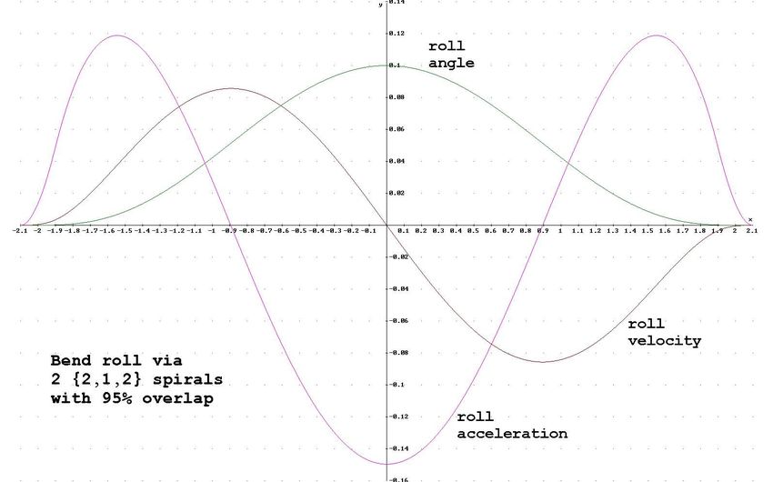
Figure 6. Roll functions for 2-{2,1} Bend with q = 0.9*a
Note with respect to equation (1) above that in railroad practice the roll angle will not normally be
more than about 0.1 radians (6 inches elevation relative to a gage of about 60 inches) and that as aBends, Jogs, And Wiggles for Railroad Tracks and Vehicle Guide Ways, Louis T Klauder Jr. 11
(Preprint, June 24, 2002)
result the tangent of the roll angle will be nearly the same as the roll angle itself. Equation (1) thus
indicates that the curvature at each point along the Bend will be approximately proportional to the roll
angle at that point and hence that the total change of track bearing angle accomplished by a Bend will
be approximately proportional to the integral of roll angle over the length of the Bend. Comparing the
above three figures it can be observed that the area under the roll angle curve, and thus also the total
turn angle of the Bend, decreases as q decreases. Note also that q cannot be lowered to 0, since
with q = 0 the constituent roll accelerations would cancel and there would be no curvature at all.
Illustrations of track shapes derived from roll functions are provided for some of the roll functions that
are defined below. However, the basic idea that applies in all cases can be seen via comparison of the
plots of roll angle in Figure 2 and superelevation in Figure 3 with the plots of curvature and alignment
in Figure 3.
The roll function family described above could be used in practice. There are some small unaesthetic
inflections in the roll acceleration function in Figure 5 near s = 0, but they would have little effect on
the dynamic performance of a corresponding Bend. However, we will present another approach that
appears more attractive.
4. Constructing the roll acceleration for a Bend by inserting a factor.
In order to find another way to construct a roll acceleration function that will generate a Bend, we
compare the simple spiral roll acceleration of Figure 2 with the Bend roll acceleration of Figure 4. In
Figure 2 the roll acceleration crosses the s axis at s = 0 as a result of the presence of the factor s in
equation (2). Looking at Figure 4 we observe that the roll acceleration function for a Bend crosses the
s-axis once to the left of s = 0 and again to the right of s = 0. We can cause an s-axis crossing at
s = - f by inserting into equation (2) a factor of (s + f ), we can cause another s-axis crossing at s = f
by inserting a factor of (s – f ), and we can remove the crossing at s = 0 by dropping the factor of
s. The resulting roll acceleration formula can be written as
d2
2
r _ angle( s ) = j ⋅ ( s + a) 2 ⋅ ( s − a ) 2 ⋅ ( s + f ) ⋅ ( s − f ) (10)
ds
where j is a multiplier to be determined. This roll acceleration extends from s = - a to s = a and
is evidently symmetric about its mid point. It therefore qualifies as the roll acceleration for a Bend. We
label this roll acceleration function in accordance with the orders of its zeros as {2,2} where the first
2 indicates that there is a second order zero at each end and the second 2 indicates that there are
two first order zeros in the interior. Applying the constraint that the roll velocity must return to zero at
the end of the Bend at s = a we find that it is necessary to have f = a / 7 , and allowing a
redefinition of j the formula for the roll acceleration becomes
d2
2
r _ angle( s ) = j ⋅ (a 2 − s 2 ) 2 ⋅ (a 2 − 7 s 2 ) (11)
ds
The shapes of this roll acceleration function and of the corresponding roll velocity and roll angle
functions are illustrated in Figure 7.Bends, Jogs, And Wiggles for Railroad Tracks and Vehicle Guide Ways, Louis T Klauder Jr. 12
(Preprint, June 24, 2002)
Figure 7. Roll functions for {2,2} Bend.
It may be observed that the roll functions of Figure 7 are similar in character to their counterparts in
Figure 4.
Figures 8 and 9 show an example of a Bend alignment that was obtained by integrating equation (11)
and that connects two adjacent sections of tangent track. In this example the angle of turn between the
two tangents is 0.1 radians (= 5.73 degrees), the maximum superelevation of the track is 0.1 radians (=
about 6 inches superelevation), the balancing speed of the Bend is set as 90 mph, and the height of the
roll axis above the track is set at 8 feet..
FIGURE 8. Alignment of a Bend connecting two tangents whose bearings differ by 0.1 radians
(= 5.73 deg.) with track bank angle of 0.1 radians (about 6 inches superelevation) at the mid
point, with length such that the balance speed is 90 mph, and with the track roll axis 8 feet
above the track. The “y” axis is the symmetry line of the two tangents and the “x” axis is the base
line that passes through the point of intersection of extensions of the tangents.Bends, Jogs, And Wiggles for Railroad Tracks and Vehicle Guide Ways, Louis T Klauder Jr. 13
(Preprint, June 24, 2002)
FIGURE 9. Track roll angle versus distance along the base line for the Bend of Figure 8.
For a Bend with parameters like these it is practical to introduce three approximations that simplify the
mathematics. First, the tangent function in equation (1) is replaced by its argument (the bank angle in
radians). Second and third, when integrating the sine and cosine of the track bearing angle, b_axis(s),
to obtain respectively the “ y” and “ x” coordinates of points on the path of the roll axis, the sine of the
bearing angle is replaced by the bearing angle itself and the cosine of the bearing angle is replaced by
unity. The effect of the second and third simplifications taken together is that b_axis(s) ceases to be
the bearing angle and becomes in stead the tangent of the bearing angle. Therefore, when these
simplifications are being applied b_axis(s) will be renamed as bt_axis(s) as a reminder.
Alignments obtained based on these simplifications will differ from corresponding alignments
obtained when the integrations are carried out numerically on the conceptually correct integrands.
However, as long as roll angles and bearing angle changes do not exceed about 0.1 radians the
differences of shape will be small and will not have adverse effects on the motions of vehicles
traversing the Bends. The forgoing simplifications were used to obtain the alignment illustrated in
Figure 8.
The algebra for this simplified application is as follows. The track roll angle as a function of distance
obtained by integrating equation (11) twice can be written as
(
r _ angle( s ) = k ⋅ a 2 − s 2 )4
(12)
where k is a constant of convenience.
As a result of the third of the three approximations the integral for the “ x” coordinate of a point on the
path of the roll axis becomes trivial, and assuming the axes shown in Figure 8 we have the result
x = s. This means that the parameter s no longer measures distance along the path of the roll axis
and instead measures distance along the “ x” axis. We therefore change the parameter in equation (1)
from s to x. Continuing in the coordinate system illustrated in Figure 8, noting that the tangent of
the bearing angle along the path of the roll axis will to be antisymmetric in x, we write
g x
bt _ axis (x ) = ⋅ dt ⋅ r _ angle(t )
v 2 ∫0
(13)
=
(
g ⋅ k ⋅ x ⋅ 315 ⋅ a 8 - 420 ⋅ a 6 ⋅ x 2 + 378⋅ a 4 ⋅ x 4 - 180 ⋅ a 2 ⋅ x 6 + 35 ⋅ x 8 )
315·v2
Pursuant to the second of the simplifications, the offset of the path of the roll axis from the base line
(i.e., along the “ y” axis in Figure 8) is given by the integralBends, Jogs, And Wiggles for Railroad Tracks and Vehicle Guide Ways, Louis T Klauder Jr. 14
(Preprint, June 24, 2002)
y _ axis(x ) = ∫ dt ⋅ bt _ axis(t )
x
(14)
−a
=
( )
- g⋅ k ⋅ 193⋅ a10 − 315⋅ a8 ⋅ s2 + 210⋅ a6 ⋅ s4 - 126⋅ a4 ⋅ s6 + 45⋅ a2 ⋅ s8 − 7⋅ s10
630⋅ v2
As already noted, with the path of the roll axis defined by equation (14) the compass bearing along it is
given by
d
b _ axis ( x) = arctan y _ axis ( x) = arctan( bt _ axis ( x) ) (15)
dx
Returning to the formula for the displacement of the Bend from the base line, it may be observed that
expression (14) is zero at each end of the Bend. To obtain the “ y” coordinates of points on the path of
the roll axis relative to the base line through the intersection of the two tangents as shown in Figure 8 it
is necessary to add the “ y” dimension from the base line to the points where the Bend meets the
tangents, namely
turn
tan ⋅a (16)
2
where turn denotes the compass bearing of the second tangent relative to the first tangent. The track
alignment is obtained from the path of the roll axis by subtracting the overhang illustrated in Figure 1,
namely
o _ hang ( x) = h ⋅ sin ( r _ angle( x) ) (17)
where h represents the height of the roll axis above the track. Thus with the axes shown in Figure 8,
the formula for the “ y” coordinate of a point on the track becomes
turn
y _ track ( x) = y _ axis ( x) + a ⋅ tan − h ⋅ sin (r _ angle ( x) ) (18)
2
The primary constraint is that turn angle of the Bend be equal to turn. In light of equation (15) the
equation that expresses that constraint is
turn
bt _ axis (a ) = tan (19)
2
and solving that equation for the multiplier k we obtain
turn 2
315 ⋅ tan ⋅v
2
k= (20)
128 ⋅ a 9 ⋅ g
There are two secondary constraints that place lower limits on the value of the half length a. One is
that the roll angle of the track not exceed a maximum value denoted max_roll. That constraint is
expressed by the equation r _ angle(0) = max_ roll . Solving that equation for a provides a lowerBends, Jogs, And Wiggles for Railroad Tracks and Vehicle Guide Ways, Louis T Klauder Jr. 15
(Preprint, June 24, 2002)
limit of
turn
315 ⋅ v 2 ⋅ tan
2
a _ roll _ lim = (21)
128 ⋅ g ⋅ max_ roll
The other secondary constraint is that the roll velocity along the track not exceed a value
corresponding to the maximum allowed value of the twist of the track. That constraint is expressed by
the equation
−a
r _ veloc = max_ r _ veloc (22)
7
where r_veloc(x) is the derivative of r_angle(x) with respect to x. Solving that equation for a
the corresponding lower limit on the value of a is found to be
turn
9 ⋅ (308700)1 / 4 ⋅ v ⋅ tan
2
a _ twist _ lim = (23)
98 ⋅ g ⋅ max_ r _ veloc
The formulae for the minimum value of the half length, a , that follow from the secondary constraints
on maximum roll angle and maximum roll velocity show simple dependence on the turn angle, turn,
the balancing speed, v, and on the maximum roll angle or the maximum roll velocity. It is generally
desirable to choose a value for a that is greater than both of the lower limits if the circumstances of
the right of way so allow.
To obtain the distance along the track as a function of the “ x” coordinate along the base line it is
necessary to carry out a numerical integration. In light of equations (3) and (15) the formula is
x 1
s _ track ( x) = ∫ dz ⋅ (24)
0 d
cosarctan(bt _ axis ( z ) ) − arctan h sin (r _ angle( z ) )
dz
Stepping back to compare the two forms of Bend at which we have looked, it can be noted that the roll
acceleration formula in equation (11) is simpler than equation (9) that governs Figures 4, 5, and 6
partly because it does not have a parameter like the parameter q of equation (9) that provides an
additional degree of freedom for constructing Bend shapes. Comparing the roll acceleration function of
Figure 7 with that of Figure 6 we can observe that the turn angle of a Bend derived from the roll
acceleration function of Figure 7 could be increased if we could find a convenient way to put a smooth
dip in the magnitude of the roll acceleration near s = 0. We can do that by adding to equation (11) a
factor of (1 + q s2) where q is an adjustable parameter. Again applying the constraint that the roll
velocity should be zero at the end of the Bend and solving for the constant multiplier in terms of the
maximum value of the roll angle we obtain the formula
- 120·max_roll·(a + s)2 (a - s)2 (a4 q + 3·a2 (1 - q·s2 ) - 21·s2 )·(q·s2 + 1)
2 2
d r/ds = ————————————————————————————— (25)
a8·(a4·q2 + 22·a2·q + 45)Bends, Jogs, And Wiggles for Railroad Tracks and Vehicle Guide Ways, Louis T Klauder Jr. 16
(Preprint, June 24, 2002)
Setting the parameter q to zero causes equation (25) to become equivalent to equation (11).
Increasing the parameter q from zero produces a family of Bends with increasing total turn angles.
Figure 10 illustrates the roll motions obtained with a = 2.0, with the maximum roll angle set to 0.1
radians, and with q set to 5.0.
Figure 10. Roll functions for hybridized {2,2} Bend with q = 5.0.
While formula (25) could be used as the basis for a family of Bend shapes, it will be preferable in
practice to use the more general approach that will be set forth in Section 9 below.
5. Constructing the roll acceleration for a Jog by overlapping three spirals
The term Jog as used herein refers to an alignment shape that begins tangent to one straight line, that
moves smoothly away from that line toward a second straight line that is parallel to but not collinear
with the first one, that ends tangent to the second line, and that is antisymmetric about its mid point. A
crossover between adjacent parallel straight tracks provides an example of what a Jog looks like.
Recall that the roll acceleration for the 2-{2,1} Bend was formed by adding the roll acceleration of a
spiral to the roll acceleration of another spiral with partial overlap. Analogously, by adding the roll
acceleration of a {2,1} spiral to that of a 2-{2,1} Bend with the same partial overlap we obtain the roll
acceleration of a 3-{2,1} Jog. The corresponding formula is
d2r/ds2 = - BOX(-a - q, s, a - q)·j·(s + q) (s + q - a)2 (s + q + a)2
+ 2 BOX(-a , s, a )·j·(s ) (s - a)2 (s + a)2
- BOX(-a + q, s, a + q)·j·(s - q) (s - q - a)2 (s - q + a)2 (26)Bends, Jogs, And Wiggles for Railroad Tracks and Vehicle Guide Ways, Louis T Klauder Jr. 17
(Preprint, June 24, 2002)
Because of the complexity of this formula it was not possible with the computing resources available
during preparation of the present article to obtain a general formula for the values of s at which the
magnitude of the roll associated with equation (26) has its maximum values. However, that would not
prevent use of the formula in design work. A sense of what the roll functions look like can be gleaned
from Figures 11 and 12 in which the functions are evaluated for a = 2, j = 0.1, and q = 1.4 (65%
overlap) and 2.2 (45% overlap) respectively.
Figure 11. Roll functions for 3-{2,1} Jog with 65% overlap.Bends, Jogs, And Wiggles for Railroad Tracks and Vehicle Guide Ways, Louis T Klauder Jr. 18
(Preprint, June 24, 2002)
Figure 12. Roll functions for 3-{2,1} Jog with 45% overlap.
For overlap values below 45% or above 65% the roll acceleration curves become less smooth and
hence presumably less desirable for design of Jogs for railroad track. Even with the parameters of
Figures 11 and 12 that are usable, one can observe unaesthetic inflections in the acceleration curves.
The combination of that lack of smoothness and the mathematical complexity of the algebra of
equations like equation (26) make Jogs of the above type unappealing in comparison to those that are
presented in the following Sections.
6. Constructing the roll acceleration for a Jog by inserting a factor.
We now look at a second way to form the roll acceleration function for a Jog. Just as each of the Bend
formulae has one more root (or s-axis crossing) than the corresponding Spiral formula, so, each of the
three curves (roll acceleration, roll velocity, and roll angle) defining the roll motion of a Jog needs to
have one more root than the corresponding curve for a Bend. Starting from equation (10) which was
the initial equation for a Bend and which is symmetric about the mid point, we can both add another
root and make the resulting function antisymmetric by inserting a factor of s so that the added root is
at the mid point of the function. The result is
d2
2
r _ angle( s ) = j ⋅ ( s + a) 2 ⋅ ( s + f ) ⋅ s ⋅ ( s − f ) ⋅ ( s − a ) 2 (27)
ds
where f is between 0 and a. Integrating that equation twice to obtain the formula for the change
in roll angle over the length of the Jog and requiring that the change in roll angle be zero at the end of
the Jog, we find that we must set f = a . If we then solve for the constant multiplier in terms of
3
the maximum roll angle in the Jog, max_roll, the formula for the multiplicative Jog becomesBends, Jogs, And Wiggles for Railroad Tracks and Vehicle Guide Ways, Louis T Klauder Jr. 19
(Preprint, June 24, 2002)
d2 - 59049⋅ max_roll⋅ s ⋅ (a 2 − s 2 ) 2 (a 2 − 3 s 2 )
r _ angle (s) = (28)
ds 2 512 a 9
Figure 13 illustrates the shapes of the roll functions for the multiplicative Jog.
Figure 13. Symmetric (i.e., antisymmetric) Jog roll functions via 5 factor roll acceleration.
The overall turn angle of the antisymmetric Jog can be seen to be zero because the curve for the roll
angle is antisymmetric about the mid point of the Jog.
7. Jogs as Shapes for Turnouts and Crossovers
This Section configures a jog intended to serve as the alignment for a crossover between two parallel
tangent (i.e., straight) tracks. As the track bearing angles relative to the two tangents and the track roll
angles are small, it is reasonable to use the simplified treatment set forth in Section 4 above.
The formula for the roll angle of the symmetric Jog as a function of length along the track is obtained
by integrating equation (28) twice and can be written in the form
(
r _ angle( s ) = − k ⋅ s ⋅ a 2 − s 2 )
4
(29)
where k is a constant of convenience. The corresponding form of equation (28) for the roll
acceleration isBends, Jogs, And Wiggles for Railroad Tracks and Vehicle Guide Ways, Louis T Klauder Jr. 20
(Preprint, June 24, 2002)
(
r _ accel ( s ) = − 24 ⋅ k ⋅ s ⋅ a 2 − s 2 ) (3 ⋅ s
2 2
− a2 ) (30)
The minus sign is inserted so that for k positive, at the left end of the Jog where s < 0 , the initial
bank and turn will be positive which is interpreted as being to the left.
Applying the first small angle approximation, the integral for the tangent of the bearing angle along the
path of the roll axis versus distance, x , along the tangents becomes
g x
bt _ axis(x ) = 2 ⋅ ∫ dt ⋅ r _ angle(t ) =
g ⋅k ⋅ a2 - x2 ( )
5
(31)
v −a 10·v2
Applying the second small angle approximation, the integral for the coordinate of a point on the roll
axis along a “ y” axis normal to the two tangents and with zero value mid way between them is
y _ axis(x ) = ∫ dt ⋅ bt _ axis(t )
x
(32)
0
g ⋅ k ⋅ x ( 693 a 10 − 1155 a 8 x 2 + 1386 a 6 x 4 − 990 a 4 x 6 + 385 a 2 x 8 − 63 x10 )
=
6930 v 2
In this situation the primary constraint is that the lateral displacement over the length of the Jog,
denoted jog_dist, should equal the specified distance between the centerlines of the two parallel
tangent tracks. With the roll angle zero at each end of the Jog there is no overhang at either end, and
this constraint takes the form
jog _ dist
y _ axis (a ) = (33)
2
Solving that constraint for k we find
3465 ⋅ jog _ dist ⋅ v 2
k= (34)
256 ⋅ g ⋅ a 11
The secondary constraints are that the roll angle and twist of the track should nowhere exceed the
respective limits chosen for those two properties. (The roll velocity determines the track twist.)
The maximum value of roll angle occurs at s = -a/3 and s = a/3 so that this constraint is expressed
as
r _ angle(− a / 3) = max_ roll (35)
and the value of shape half length such that the maximum magnitude of the roll angle is max_roll is
found to be given byBends, Jogs, And Wiggles for Railroad Tracks and Vehicle Guide Ways, Louis T Klauder Jr. 21
(Preprint, June 24, 2002)
4 ⋅ 1155 ⋅ jog _ dist ⋅ v
a _ roll _ lim = (36)
81 ⋅ g ⋅ max_ roll
The magnitude of the roll velocity has its maximum value at s = 0 and the value of the shape half
length such that the magnitude of the roll velocity there equals max_r_veloc is found to be given by
6930 ⋅ jog _ dist 1 / 3 ⋅ v 2 / 3
1/ 3
a _ twist _ lim = (37)
8 ⋅ g 1 / 3 ⋅ max_ r _ veloc1 / 3
Both of the above expressions for the half length are evaluated, and the larger value is used so that both
of the secondary constraints are satisfied.
Both formulae for the Jog’s half length show that the length of the Jog will depend in a simple way on
the balancing speed, v, the Jog’s lateral displacement, jog_dist, and either the maximum bank angle,
max_roll, or the maximum roll velocity, max_r_veloc.
Since we are looking here at crossovers we need to take account of the fact that physical crossovers
begin and end with physical track switches. Physical track and guide way switch design is an immense
field in which many concepts for balancing cost and performance have been developed. What is noted
here is that costs of constructing and maintaining a switch are increased when there is an increase in
the length of the assembly that must move when the setting of the switch is changed. That length
increases when there is an increase in the track length over which geometry prevents a guide rail or
rails from simultaneously being in the working location for the both routes. This means that it is
desirable to arrange to have the initial lateral separation of the “ diverging” path from the “ through”
path develop as rapidly as vehicle dynamics will allow. We have observed that raising the height of the
vehicle roll axis above the track is always dynamically beneficial. However, raising the vehicle roll
axis also causes an increase in the distance from the start of a Jog to the point at which the Jog reaches
a given lateral displacement toward the final tangent. Therefore, in contrast to the application of the
Bend in Section 4 above, for this application of a Jog as a crossover the roll axis is not raised and the
path of the track is given by equation (32) itself. We thereby make some sacrifice of dynamic
performance in order to reduce the cost of the crossover.
Figure 14 illustrates such a crossover for the conditions that the two adjacent sections of tangent track
have a centerline separation of 20 feet, that the maximum superelevation in the crossover is 0.05
radians (about 3 inches superelevation), and that the balance speed of the crossover is 90 mph. The
crossover extends for 781 feet in each direction from the center of symmetry. Figure 16 shows the
track roll angle profile corresponding to Figure 14 as given by equation (30). (Formulae for Figures 15
and 17 are presented following Figure 17.)Bends, Jogs, And Wiggles for Railroad Tracks and Vehicle Guide Ways, Louis T Klauder Jr. 22
(Preprint, June 24, 2002)
Figure 14. A Jog constructed from the roll acceleration of equation (30) which has a 2nd order
zero at each end. This Jog is configured as a crossover between tangent tracks with centerline
spacing of 20 ft, with maximum roll angle of 0.05 radians (corresponding to maximum
superelevation of about 3 inches), and with dimensions chosen so that the balancing speed is 90
mph. The total length of the crossover measured along the tangents is 1,562 ft. (Note that in
North American practice crossovers are not usually designed for high speed operation and do
not usually include superelevation.)
FIGURE 15. A Jog constructed from the roll acceleration of equation (30) with a 1st order zero at
each end. Other design parameters are the same as those for Figure 14. Because the roll angle
builds more quickly at each end than is the case when the roll acceleration has 2nd order zeros at
the ends, this crossover is shorter than the one in Figure 14. The total length of this crossover
measured along the tangents is 1,424 ft.
FIGURE 16. Track roll angle for Jog of Figure 14.Bends, Jogs, And Wiggles for Railroad Tracks and Vehicle Guide Ways, Louis T Klauder Jr. 23
(Preprint, June 24, 2002)
FIGURE 17. Track roll angle for Jog of Figure 15.
We look next at the rationale of Figures 15 and 17. As noted at the end of Section 2 above, when the
roll axis is not raised above the plane of the track it is reasonable to look at roll acceleration functions
that have 1st rather than 2nd order zeros at the ends. Starting with the counterpart of equation (27) but
with 1st order rather than 2nd order zeros at s = - a and s = a and repeating the sequence of steps
that lead from equation (27) to equation (28), one finds that the counterpart of equation (28) with a 1st
order zero at each end is
d2
r _ angle ( s ) =
(
343 7 ⋅ max_ roll (a + s )(a − s ) 3 a 2 − 7 s 2 ) (38)
ds 2 36 a 7
The formula for the roll angle of the symmetric Jog obtained by integrating equation (38) twice can be
written in the form
(
r _ angle ( s ) = − k s a 2 − s 2 )
3
(39)
where k is another constant of convenience.
Applying the simplified treatment as in the previous case the integral for the tangent of the bearing
angle versus distance, x , along the tangents becomes
g x
bt _ axis(x ) = 2 ⋅ ∫ dt ⋅ r _ angle(t ) =
g⋅ k a2 - x2 ( )
4
(40)
v −a 8 v2
Applying the second small angle approximation, the integral for the distance along a “ y” axis normal
to the two tangents is
y _ axis (x ) = ∫ dt ⋅ bt _ axis(t )
x
(41)
0
=
(
g ⋅ k ⋅ x 315 a 8 − 420 a 6 x 2 + 378 a 4 x 4 − 180 a 2 x 6 + 35 x 8 )
2520 v 2
The primary and secondary constraints and the manner in which they are used to determine k and a
are the same as in the previous case. The solution for k is
315 ⋅ jog _ dist ⋅ v 2
k = (42)
32 ⋅ a 9 gBends, Jogs, And Wiggles for Railroad Tracks and Vehicle Guide Ways, Louis T Klauder Jr. 24
(Preprint, June 24, 2002)
The lower limit for a such that the max_roll constraint is satisfied is
9 ⋅ (77175)
1/ 4
⋅ jog _ dist ⋅ v
a _ roll _ lim = (43)
98 ⋅ g ⋅ max_ roll
and the lower limit for a such that the max_r_veloc constraint is satisfied is
630 ⋅ jog _ dist 1 / 3 ⋅ v 2 / 3
1/ 3
a _ twist _ lim = (44)
4 ⋅ g 1 / 3 ⋅ max_ r _ veloc1 / 3
The constraints on the Jog’ s half length show the same dependence as before on the balancing speed,
the Jog’ s lateral displacement, and on the maximum bank angle or maximum roll velocity but with
different constant factors.
Figure 15 illustrates a crossover based on the above formulae for the conditions that the two adjacent
sections of tangent track have a centerline separation of 20 feet, that the maximum superelevation in
the crossover is 0.05 radians (about 3 inches superelevation), and that the balance speed of the
crossover is 90 mph. The crossover extends for 712 feet in each direction from the center of symmetry.
Figure 17 shows the track roll angle profile corresponding to Figure 15 as given by equation (39).
In contemporary North American railroad practice turn-outs from tangent tracks do not incorporate
superelevation and therefore do not have defined balancing speeds. Construction of a switch that
incorporated superelevation as prescribed by the formulae of this Section would require progressive
lowering of the rail seats of the low rail of the diverging route and would require a novel machining of
the “ point” for the through route. The points would also be longer than the points of conventional
railroad switches.
8. Constructing the roll acceleration for a Wiggle by inserting a factor
The term Wiggle as used herein refers to an alignment shape that begins tangent to some straight line,
that makes a smooth lateral excursion away from and then back toward that straight line, that ends
again tangent to that straight line, and that is symmetric about its mid point. (We will see in Section 9
below that asymmetry can be accommodated by addition of higher order shapes.) As noted in the
introduction, a Wiggle can be an effective way for an otherwise straight alignment to circumvent a
local obstruction that intrudes from one side. We construct a roll acceleration formula that can exhibit
the features of a Wiggle by adding another linear factor to the Jog roll acceleration formula in equation
(27). The initial formula is
d2
2
r _ angle ( s ) = j ( s + a) 2 ( s + p) ( s + f ) ( s − q ) ( s − i ) ( s − a ) 2 (45)
ds
The parameters p and i are eliminated by applying the constraints that the roll velocity and roll
angle both return to zero at s = a. The asymmetry of the resulting roll acceleration polynomial is
controlled by (f – q). It is therefore convenient to replace f and q by the new variables b = (f +Bends, Jogs, And Wiggles for Railroad Tracks and Vehicle Guide Ways, Louis T Klauder Jr. 25
(Preprint, June 24, 2002)
q)/2 and c = (f – q)/2. We want these shapes to be symmetric so that c is set to zero and drops out.
This makes the roll acceleration a polynomial in s that depends on j, a, and b.
The following figures illustrate the shape of the roll angle function for two values of the parameter b.
Figure 18. Symmetric roll functions via 6 factor roll acceleration with b = 1.0.Bends, Jogs, And Wiggles for Railroad Tracks and Vehicle Guide Ways, Louis T Klauder Jr. 26
(Preprint, June 24, 2002)
Figure 19. Symmetric roll functions via 6 factor roll acceleration with b = 1.1.
Looking in Figure 18 at the areas between the roll angle curve and the distance axis one can see that
the amounts of curvature to the right and to the left are approximately equal so that the total angle of
turn over the length of the shape will approximate the desired value of zero. By way of contrast, the
roll angle curve of Figure 19 is biased to one side so that the resulting shape will look much like a
Bend and not much like a Wiggle.
The roll angle function corresponding to equation (45) is a 10th order polynomial. To obtain a closed
form algebraic expression for the constraint that the compass bearing of the Wiggle be the same at the
end as at the beginning would require putting that 10th order polynomial roll angle function into
equation (1) and then obtaining the compass bearing angle as the integral of equation (1) in closed
form. As that is considered impossible we will provide an illustration using the simplified method
described in Section 4 above. The formula for the tangent of the bearing angle on the path of the roll
axis is then available in closed form. Imposing the requirement that the tangent of the bearing angle be
the same at the end as at the beginning fixes the value of b, and in the context of the simplified
treatment the equation for the roll acceleration of a Wiggle (with j redefined) becomes
d2
2
r _ angle ( s ) = j (a 2 − s 2 ) 2 (a 4 − 18 a 2 s 2 + 33 s 4 ) (46)
ds
What comes next is an example of application of a Wiggle to avoid a single obstacle in an otherwise
straight section of track. The illustration makes use of the mathematical simplifications that were
explained in Section 4 above. The roll angle function corresponding to equation (46) can be written as
r _ angle ( s ) = k ( a 2 − s 2 ) 4 (11 s 2 − a 2 ) (47)
where k is a constant of convenience. Integrating the simplified version of equation (1) yields
− g ⋅ k ⋅ x ⋅( a 2 − x 2 )5
bt _ axis ( x) = (48)
v2
and evaluating the simplified form of the integral for y_axis yields
g ⋅ k ⋅ ( a 2 − x 2 )6
y _ axis ( x) = (49)
12 v 2
The “ y” coordinate along the path of the track is
y _ track ( x) = y _ axis ( x) − cos (arctan(bt _ axis ( x) ) )⋅ o _ hang ( x) (51)
where o_hang(x) is the overhang as described previously.
The primary constraint is that the lateral excursion from the general tangent have a specified value that
we denote by swing_dist and takes the formBends, Jogs, And Wiggles for Railroad Tracks and Vehicle Guide Ways, Louis T Klauder Jr. 27
(Preprint, June 24, 2002)
y _ track (0) = swing _ dist (52)
It is evident from equation (48) that bt_axis(0) = 0. Therefore when equation (51) is used in equation
(52) the cosine factor is unity and can be dropped. To get the constraint into a form that can be solved
algebraically we can introduce another approximation that is in keeping with the simplified treatment.
Namely, in the equation for the overhang we replace the sine of the roll angle by the roll angle itself
and write
o _ hang ( x) = h ⋅ r _ angle ( x) (50)
We can then solve for k and find
12 ⋅ swing _ dist ⋅ v 2
k = 10 2 (53)
a ( a g + 12 ⋅ h ⋅ v 2 )
There are two secondary constraints. One is that the maximum roll angle that occurs at s = 0 not
exceed a specified value we denote as max_roll. The lower limit for a obtained by solving that
constraint is
2 ⋅ 3 ⋅ v ⋅ (h ⋅ max_ roll + swing _ dist )
a _ roll _ lim = (54)
g ⋅ max_ roll
The other secondary constrain is that the maximum roll velocity (which corresponds to maximum
allowed track twist) which occurs at − a ⋅ 3 − 4 3 not exceed a value we denote as
11 33
max_r_veloc. The lower limit for a obtained by solving that constraint is
h theta
a _ twist _ lim = − 4 ⋅ − 1 ⋅ v ⋅ sin (55)
g 3
where
1517158400 ⋅ 3 454246400
−1 ⋅ (h ⋅ g ) ⋅ swing _ dist ⋅
526153617 + 58461513
theta = arcsin (56)
h ⋅ max_ r _ veloc ⋅ v
2
The values used for the example illustrated in Figures 20 and 21 are: swing distance = 20.0 feet;
balancing speed = 90 mph; roll axis height = 8.0 feet; maximum roll velocity corresponding to a
maximum change of cross level in 62 feet = 1.2 inches; and the acceleration of gravity = 32.17
feet/second_squared. With the selected parameters the roll angle does not get as large as the typical
limit of 0.1 radians. While the alignment given by this simplified construction is not identical to the
alignment that would be obtained if all of the trigonometric functions of the method were fully
evaluated, its utility and dynamic characteristics will be just as good as those of a correspondingBends, Jogs, And Wiggles for Railroad Tracks and Vehicle Guide Ways, Louis T Klauder Jr. 28
(Preprint, June 24, 2002)
construction with the trigonometric functions fully evaluated. However, if this simplified treatment is
used in practice, the engineer will need to be aware that the relationship between curvature and
superelevation is slightly different than normal and will need to take account of that when establishing
authorized speeds.
FIGURE 20. Illustration of a simplified Wiggle that swings 20.0 feet laterally to avoid an obstacle
along what is otherwise straight track.
FIGURE 21. The superelevation (assuming a 60.0 inch gage) of the same Wiggle as in Figure 20.
9. Simplification and Generalization by means of Gegenbauer Polynomials
We next look again at equation (11)
d2
r _ anglebend ( s ) = j ⋅ (a 2 − s 2 ) 2 ⋅ (a 2 − 7 s 2 ) (11)
ds 2
that gives the roll acceleration function for a Bend. That equation is integrated once to obtain the roll
velocity function and a second time to obtain the roll angle function. The fact that we need to work
with the integral of (a2 – s2)2 times a polynomial suggests a check to see if one of the classical
orthogonal polynomial families has a weighting function that can take the form (a2 – s2)2. Consulting
a treatise on orthogonal polynomials such as Reference 6, one finds that the Gegenbauer polynomials
denoted C n(α ) (x ) are defined with respect to the weighting function (1 - x2) - ½) which with suitable
choices for the variables can take the form with which we are dealing. Starting with equation 22.13.2
of Reference 6, defining m = - ½ , scaling the variable of integration so that the limits of integration
are from - a to a, and working with n one can obtain the relation
s
( )C
2 m (m +1 / 2 ) (
(t / a ) = − (2m + 1) a − s
2 2
)(m +1)
C n(m−1+3 / 2 ) (s / a )
∫ dt ⋅ a − t
2
(57)
n(2m + 1 + n )
n
−a aBends, Jogs, And Wiggles for Railroad Tracks and Vehicle Guide Ways, Louis T Klauder Jr. 29
(Preprint, June 24, 2002)
It may be noted that C n(α ) (x ) is a polynomial of order n that is an even or odd function of x depending
on whether n is an even or odd integer.
Looking at the explicit expression for C 2(5 / 2 ) (s / a ) and introducing a constant j2 it is easy to verify
that equation (11) that gives the roll acceleration for a Bend can be rewrite as
d2
ds 2
( 2
)
r _ anglebend ( s ) = j 2 ⋅ a 2 − s 2 C 2(5 / 2 ) (s / a ) (58)
In the same way one can verify that the right sides of equations (2), (28), and (46) that give the roll
acceleration functions for a Spiral, for a Jog, and for a Wiggle can be written as
(
jn ⋅ a 2 − s 2 ) C(
m
n
m +1 / 2 )
(s / a ) , n 1, (59)
with n = 1, 3, and 4 respectively and with jn denoting the weighting coefficient for the order n
contribution. We are therefore lead to look upon a series of terms of the form of expression (59) with
n >= 1 as the roll acceleration of defining a general connecting shape in which the curvature varies
with distance over the length of the shape.
By virtue of equation (57) the equation for roll velocity obtained by integrating expression (59) once
will contain a factor of (a2 – s ) . For terms with n >= 2 the contributions to the roll angle obtained
2 3
by integrating a second time will contain a factor of (a2 – s2)4. Thus the two constraints that the roll
velocity and roll angle both return to zero at s = a will be satisfied automatically for terms with n
>= 2.
Applying equation (57) twice the contribution of a term with n >= 2 to the roll angle is found to be
j n (2m + 1) (2m + 3) (a 2 − s 2 ) ( m+ 2) ( m+5 / 2)
C n−2 (s / a) (60)
n (n − 1) (2m + 1 + n) (2m + 2 + n) a2
It was pointed out in Section 8 that with the Wiggle roll acceleration given by equation (46) or
( )
equivalently by j 4 ⋅ a 2 − s 2 C 4(5 / 2 ) (s / a ) the total compass bearing change over the length of the
2
Wiggle will vanish as it should if the “ simplified” treatment is used but not if the trigonometric
integrands are fully evaluated. Therefore, in a “ full” treatment that includes even order Gegenbauer
terms with n >= 4 it is necessary to include at least a little n = 2 or Bend component and to adjust
the strength of that component so that the net change of compass bearing over the length of the shape
has the required value.
As a rule-of-thumb, the “ simplified” method can be used with no problem for a shapes that connects to
a tangent at each end, and the “ full” method should be used for any shape that connects at one or both
ends to a curved arc.
It should be noted that equation (57) holds for non-integral values of m provided that m > -1. As
an example, choosing m = 2.5 would cause the roll acceleration to rise from zero more slowly at
each end of the shape but would then mean that roll acceleration values would be greater in the interior
of the distance covered by the shape. Choosing m = 1.5 would have the opposite effects.You can also read