Electron diffraction by vacuum fluctuations - IOPscience
←
→
Page content transcription
If your browser does not render page correctly, please read the page content below
PAPER • OPEN ACCESS

Electron diffraction by vacuum fluctuations
To cite this article: Valerio Di Giulio and F Javier García de Abajo 2020 New J. Phys. 22 103057

View the article online for updates and enhancements.

                               This content was downloaded from IP address 46.4.80.155 on 21/11/2020 at 12:24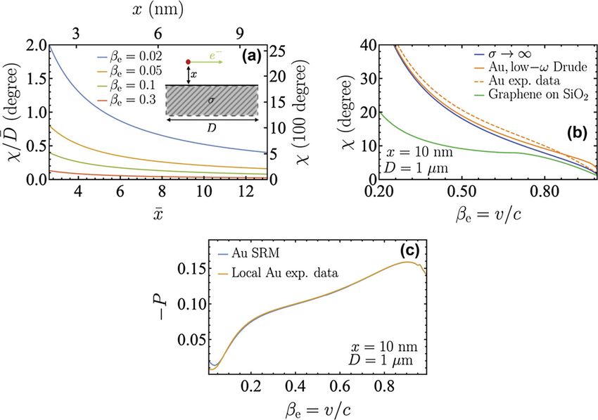
New J. Phys. 22 (2020) 103057                                                                https://doi.org/10.1088/1367-2630/abbddf

                                 PAPER

                                 Electron diffraction by vacuum fluctuations
O P E N AC C E S S

                                 Valerio Di Giulio1 , ∗      and F Javier Garcı́a de Abajo1 , 2 , ∗
R E C E IVE D
                                 1
8 July 2020                          ICFO-Institut de Ciencies Fotoniques, The Barcelona Institute of Science and Technology, 08860 Castelldefels (Barcelona), Spain
                                 2
                                     ICREA-Institució Catalana de Recerca i Estudis Avançats, Passeig Lluı́s Companys 23, 08010 Barcelona, Spain
R E VISE D                       ∗
28 September 2020                    Author to whom any correspondence should be addressed.

AC C E PTE D FOR PUBL IC ATION
                                 E-mail: valerio.digiulio@icfo.eu and javier.garciadeabajo@nanophotonics.es
2 October 2020
                                 Keywords: electron microscopy, vacuum fluctuations, photonic nanostructures, light–matter interaction
PUBL ISHE D
29 October 2020

Original content from
                                 Abstract
this work may be used
under the terms of the
                                 Vacuum fluctuations are known to produce electron diffraction leading to decoherence and
Creative Commons                 self-interference. These effects have so far been studied as either an extension of the
Attribution 4.0 licence.
                                 Aharonov–Bohm effect in front of a planar perfect conductor or through path integral analysis.
Any further distribution
of this work must                Here, we present a simpler, general, and rigorous derivation based on a direct solution of the
maintain attribution to          quantum electrodynamic aloof interaction between the electron and a material structure in the
the author(s) and the
title of the work, journal       temporal gauge. Our approach allows us to study dissipative media, for which we show examples
citation and DOI.
                                 of electron wave function shaping due to the interaction with real-metal surfaces. We further
                                 present a proof of the relation between the phase associated with vacuum fluctuations and the
                                 Aharonov–Bohm effect produced by the image self-interaction that is valid for arbitrary
                                 geometries. Besides their fundamental interest, our results could be useful for on-demand
                                 patterning of electron beams with potential application in nondestructive nanoscale imaging and
                                 spectroscopy.

                                 1. Introduction

                                 On-demand coherent manipulation of the transverse electron wave function in electron beams is of
                                 fundamental interest to improve spatial resolution in transmission electron microscopes. The problem can
                                 be simply stated as the question of how to introduce a position-dependent phase in the electron wave
                                 function. Currently, energetic electron beams can be focused down to sub-Ångstrom spots by phase shaping
                                 their transverse wave functions using electrostatic and magnetostatic lenses, which produce macroscopic
                                 changes in the phase profile to correct aberrations in the electron optics. Recently, perforated transmission
                                 phase plates have been successfully demonstrated to create beams carrying high values of angular
                                 momentum [1], while dynamical phase patterning has been explored with the use of pixelated electrostatic
                                 plates [2]. An alternative possibility consists in exploiting photon-electron interactions, which can affect the
                                 transversal phase as demonstrated for example in the Kapitza–Dirac effect [3, 4], and also in the recently
                                 demonstrated angular momentum transfer between light and electron beams [5]. This approach has been
                                 theoretically proposed to be useful for aberration correction [6], although it involves the emission or
                                 absorption of real photons, therefore producing inelastic rather than elastic diffraction.
                                     In a related context, vacuum fluctuations can also induce a phase modulation without the exchange of
                                 real photons, an effect that has been theoretically investigated in the presence of nondissipative media [7]
                                 and is still lacking experimental confirmation to the best of our knowledge. For an electron moving parallel
                                 to a perfect conductor surface, this phase has been explained as arising from the Aharonov–Bohm effect [8]
                                 produced by the electron image potential [7], while an alternative derivation has been given in terms of
                                 path integrals [9]. The presence of material excitations with which the electron may interact could add new
                                 degrees of freedom to manipulate the quantum phase, although their study would be difficult to undertake
                                 using existing theoretical approaches. It should be noted that the same type of electron phase was analyzed
                                 in detail in early pioneering works in a different context related to electron microscopy and the
                                 understanding of elastic scattering by atomic crystal lattices for penetrating trajectories [10, 11]. However,
                                 the real part of the correction to the optical potential computed in these works was found to be too small in

                                 © 2020 The Author(s). Published by IOP Publishing Ltd on behalf of the Institute of Physics and Deutsche Physikalische Gesellschaft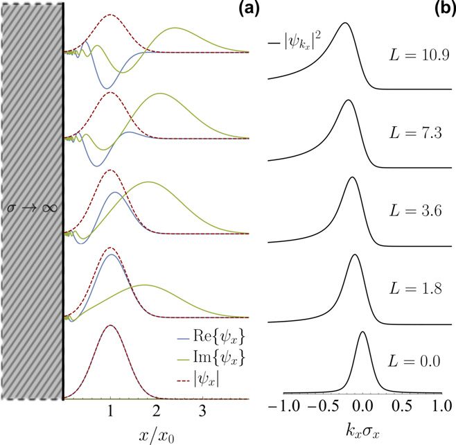
New J. Phys. 22 (2020) 103057                                                        V Di Giulio and F J Garcı́a de Abajo

samples with thickness smaller than the electron mean free path, and therefore, never experimentally
observed as far as we know. In this context, aloof trajectories may enormously increase the interaction
length, thus making this effect observable in practice.
    In this work, we present an alternative derivation of vacuum phases produced during the interaction of
electron beams with arbitrarily structured materials, enabling us to readily include the effect of material
excitations for aloof electron trajectories. In section 2, we review a quantization scheme of the
electromagnetic field in the presence of macroscopic and lossy media, extending a previous Coulomb gauge
formulation [12] to the temporal gauge, which we find more suitable to deal with the noted interaction. We
continue by showing that vacuum fluctuations induce both phase shifts and decoherence in an
Aharonov–Bohm-like configuration. In section 3, we derive a scalar quantum electrodynamics (QED)
Hamiltonian that represents to a good approximation the evolution of an electron wave function at energy
scales typical of electron microscope setups, and further provide an analytical demonstration that the
vacuum phase shift can transversally modulate the electron beam. In section 5, we discuss the phase
produced on electrons moving parallel to either perfect or real planar conductor surfaces, whereas in
section 6 we analyze far-field diffraction induced by either a planar surface or a small particle. We anticipate
that these theoretical results could be corroborated in either interference or angle-resolved experiments.
    In brief, we discuss a general theory of the interaction between fast electrons and electromagnetic modes
in the vicinity of material media, leading to the emergence of a quantum phase imprinted on the electron
transverse wave function. For aloof interaction with a planar surface, this phase is related to the
Aharonov–Bohm effect due to the image potential [7], a result that we extend to arbitrarily shaped
structures, for which we find that the quantum phase under discussion coincides with the Aharonov-Bohm
effect associated with half (i.e., the image) of the self-induced electron vector potential in a gauge with
vanishing scalar potential. We illustrate the effect that such phase has on a free electron by investigating two
different experimental scenarios: a holographic measurement in which one compares the phase of an
electron wave function component passing near a sample with the phase of another component that does
not interact with the sample; and a diffraction measurement in which the electron distribution in the
far-field Fourier plane is modified by the dependence of the imprinted phase on transverse beam
coordinates.

2. Vacuum phase shift in the presence of macroscopic media

2.1. Macroscopic QED in the temporal gauge
Macroscopic QED has been extensively developed in the Coulomb gauge [12]. However, we find it more
convenient to work in the temporal gauge (i.e., a gauge in which the scalar potential vanishes) to describe
the interaction between free electrons and the electromagnetic fields in the presence of material boundaries.
The constitutive relations connecting the frequency components of the field and vector potential operators
then reduce to (in Gaussian units)
                                                           iω
                                              Ê(r, ω) =      Â(r, ω),
                                                            c
                                              B̂(r, ω) = ∇ × Â(r, ω),

where the vector potential operator  is taken to satisfy the wave equation

                                                     ω2                   4π noise
                                ∇ × ∇ × Â(r, ω) −      (r, ω)Â(r, ω) =    ĵ (r, ω).                             (1)
                                                     c2                    c
Here, we assume a linear local nonmagnetic response that is fully captured by the complex
frequency-dependent permittivity (r, ω), which is required to satisfy causality and the Kramers–Kroning
relations. We introduce a noise current ĵnoise to describe the dissipation produced by coupling between the
electromagnetic field and matter. More precisely, we construct this current as [12]

                                   ĵnoise (r, ω) = ω  Im{(r, ω)} f(r, ω),                               (2)

where we define bosonic operators f(r, ω) and f† (r, ω) that follow the commutation relations

                              f̂ i (r, ω), f̂ i (r , ω  ) = 0,                                                   (3)

                              f̂ i (r, ω), f̂ †i (r , ω  ) = δi,i δ(r − r )δ(ω − ω  ),                        (4)

                                               2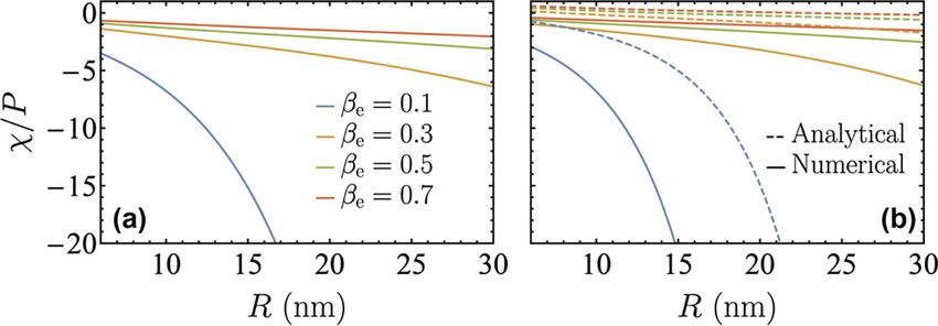
New J. Phys. 22 (2020) 103057                                                                                         V Di Giulio and F J Garcı́a de Abajo

and whose evolution is ruled by the radiation Hamiltonian [12]
                                                                          ∞
                                             Ĥrad =          d3 r              dω ω f† (r, ω) · f(r, ω).
                                                                       0

Additionally, by combining equations (2)–(4), these operators are found to satisfy the commutation
relations

                          ĵnoise
                            i     (r, ω), ĵnoise
                                            j     (r , ω  ) = 0,                                                                                   (5)

                    ĵnoise
                      i       (r, ω), (ĵnoise
                                         i    (r , ω  ))† = ω 2 Im{(r, ω)} δi,i δ(r − r )δ(ω − ω  ).                                         (6)

A formal solution of equation (1) is given by

                                            Â(r, ω) = −4πc                     d3 r G(r, r , ω)ĵnoise (r , ω),                                   (7)

where G(r, r , ω) is the electromagnetic Green tensor satisfying the relation

                                                                       ω2                         1
                                 ∇ × ∇ × G(r, r , ω) −                   (r, ω)G(r, r , ω) = − 2 δ(r − r ).                                      (8)
                                                                       c2                        c

Finally, by combining equations (5)–(7), the commutation relations of the vector potential become

                                 Âi (r, ω), Âi (r , ω  ) = 0,                                                                                   (9)

                                 Âi (r, ω), †i (r , ω  ) = 16π 2 c2 δ(ω − ω  )Im{−Gi,i (r, r , ω)},                                       (10)

where we have made used of the identity [12]

                                                                                                            1
                              d3 r Im{(r , ω)}Gi,i (r, r , ω)G∗i ,i (r , r , ω) = −               Im{Gi,i (r, r , ω)}
                                                                                                              ω2
                   i

in order to evaluate the commutator in equation (10).
    From these relations, we can work out the time-dependent commutator Âi (r, t), Âi (r , t  ) , where
Â(r, t) = eiĤrad t/ Â(r)e−iĤrad t/ , by noting that the potential frequency components are related to the
time-dependent components through the relation [13]
                                                                      ∞
                                                                            dω −iωt
                                                 Â(r, t) =                    e Â(r, ω) + h.c.,
                                                                   0        2π

which together with equations (9) and (10) lead to
                                                                         ∞
                             Âi (r, t), Âi (r , t  ) = 8ic2               dω sin ω(t − t  ) Im{Gi,i (r, r , ω)}.                           (11)
                                                                        0

As in vacuum, this commutator is a purely imaginary c-number, from which we can calculate the retarded
electromagnetic Green tensor, defined as

                                                                    −i
                                     GRi,i (r, r , t − t  ) =         Â i (r, t), Âi

                                                                                          (r , t ) θ(t − t ).                                      (12)
                                                                   4πc2

Incidentally, using the fact that G(r, r , ω) satisfies the Kramers–Kronig relations, as well as the causality
property G(−ω) = G∗ (ω), we find
                                                                                ∞
                                                 Gi,i (r, r , ω) =                 dt eiωt GRi,i (r, r , t),                                    (13)
                                                                                −∞

so the quantum retarded Green tensor coincides with the classical Green tensor defined by equation (8).

                                                              3
New J. Phys. 22 (2020) 103057 V Di Giulio and F J Garcı́a de Abajo
2.2. Vacuum phase shift
We now obtain an expression for the elastic electron amplitude under interaction with a macroscopic
quantized electromagnetic field. We consider an Aharonov–Bohm-like experiment in which the electron
wave function is split into two paths (1 and 2). Before interaction with the electromagnetic field, the system
density matrix is
ρ(t0 ) = |ψ1 (t0 )ψ1 (t0 )| + |ψ2 (t0 )ψ2 (t0 )| + |ψ2 (t0 )ψ1 (t0 )| + |ψ1 (t0 )ψ2 (t0 )| ⊗ σ(t0 ),
where σ(t0 ) stands for the initial state of the photon field at time t0 , while |ψ 1 (t0 ) and |ψ 2 (t0 ) are the
electron states in paths 1 and 2, respectively. We take the interaction between the electromagnetic field and
the electron to be described by a minimal coupling Hamiltonian in the temporal gauge, which in the
interaction picture reads
1
Ĥ(t) = − d3 r Â(r, t) · j(r, t).
c
Assuming the electron current to be well described by its classical version on each of the two electron paths,
we can write the electron density matrix at a later time t > t0 as
ρe (t) = |ψ1 (t0 )ψ1 (t0 )| + |ψ2 (t0 )ψ2 (t0 )| + |ψ2 (t0 )ψ1 (t0 )| Tr{Ŝ 2 σ(t0 )Ŝ †1 }
+ |ψ1 (t0 )ψ2 (t0 )| Tr{Ŝ 1 σ(t0 )Ŝ †2 }, (14)
(−i/) t dt Ĥ (t )
where Ŝ j = T e t0 j
is the time-ordered evolution operator for the current along path j = 1 or 2,
and we have traced out the photon degrees of freedom. The first two terms on the right-hand side of
equation (14) represent the part of the electron wave function that is not affected by interaction with the
electromagnetic field. The remaining two terms describe the coherence of the electron state. We now take
the initial photon density matrix to be in a thermal state at temperature T and use the fact that the
commutator between the vector potentials is a pure imaginary c-number (equation (11)) in order to
rigorously disregard time ordering by using Wick’s theorem [14]. By doing so, we obtain
− i tt dt Ĥj (t )
Ŝ j = eiχj e 0 = eiχj Û j ,
which, by going from t 0 = −∞ to t = ∞, leads to
Ŝ †2 Ŝ 1 T = ei(χ1 −χ2 ) Û †2 Û 1 T
with phase shifts given by
∞ t
i
χj = dt dt d3 r d3 r jj (r, t) · Â(r, t), Â(r , t ) · jj (r , t ). (15)
22 c2 −∞ −∞
Now, we use the Baker–Campbell–Hausdorff formula to recombine the evolution of the two paths, leading
to
Ŝ †2 Ŝ 1 T = ei(χ1 −χ2 ) eiϕ eP ,
where we have
∞ ∞
−i
ϕ= 2 2 dt dt d r d3 r j2 (r , t ) · Â(r , t ), Â(r, t) · j1 (r, t),
3
(16)
2 c −∞ −∞
∞ ∞
−1
P= 2 2 dt dt d3 r d3 r j1,2 (r, t) · Â(r, t)Â(r , t )T · j1,2 (r , t ), (17)
2 c −∞ −∞
and j1,2 = j1 − j2 . In this derivation, we have used the fact that Â(r, t) is linear in the field operators, and
therefore Â(r, t)T = 0 (see equations (2) and (7)), which leads to a cumulant expansion limited only to
the second-order term [15]. The phase shift given by equation (16) relates to the interference between the
two paths due to photon emission. This is clear by noticing that it appears only because of the cyclic
property of the trace, which allows us to obtain the product Ŝ †2 Ŝ 1 . In contrast, the expression in
equation (17) is guaranteed to be a real number, so it represents the total decoherence experienced by the
electron, which has been extensively studied from both theoretical [9, 16–18] and experimental [19–21]
fronts. Importantly, it should be noted that, although the impressive increase of accuracy achieved in recent
experiments served to rule out alternative theories, further decrease in experimental error is still needed to
conclusively support a physical model [18]. The path-dependent phase and decoherence, which can affect
4New J. Phys. 22 (2020) 103057 V Di Giulio and F J Garcı́a de Abajo
the fringes observed in an interference experiment, was derived as a dynamical scattering correction to the
electron virtual interaction with sample excitations in a pioneering work [10] that related it to the so-called
optical potential [11, 22, 23]. A subsequent formulation of such phase was then separately given in the
context of quantum field theory [7] assuming zero temperature and neglecting inelastic losses, while an
extension to finite temperature was later presented [15]. However, not much attention has so far been paid
to the vacuum phase shift χj (equation (15)) and the role played by dissipation and finite conductivity in
metallic structures, on which we focus here using a macroscopic QED formalism.
We find it useful to rewrite the phase shift of equation (15) in terms of the electromagnetic Green tensor
by using equations (12) and (13). This allows us to write
∞ ∞
2 ∞
χj = dt dt dω d r d3 r cos ω(t − t )
3
−∞ −∞ 0
× jj (r, t) · Re{−G(r, r , ω)} · jj (r , t ), (18)
where we have also used the Onsager reciprocity relation G(r, r , ω) = GT (r , r, ω). Now, if we consider the
electron to be a point particle traveling along the z direction with constant velocity v and fixed transverse
coordinates Rj = (xj , yj ) (different for each of the two paths j = 1 and 2), the electron current is
jj (r, t) = −ev δ(z − vt) δ(R − Rj ) ẑ, (19)
which upon insertion into equation (18) leads to the expression
∞ ∞ ω
2e2 ∞
χj = dω dz dz cos (z − z ) Re{−Gz,z (Rj , z, Rj , z , ω)} (20)
0 −∞ −∞ v
for the impact-parameter-dependent electron phase shift. This result clearly emphasizes the fact that the
quantum phase is the integral of a nonresonant quantity (the real part of the Green tensor), and thus it is
expected to be small, although the numerical examples discussed below reveal a measurable effect. In more
physical terms, the electron has to undergo an even number of virtual inelastic processes during its
interaction with the sample before recovering its initial energy, so the phase change is at least a
second-order process (indeed it arises from a commutator), although its effect is accumulated over an
infinite number of electromagnetic modes that renders it non-negligible. We also remark that the phase
does not depend on how the electromagnetic modes are populated, so it takes the same value if the sample
starts from the ground state or from an excited state.
For completeness, we calculate the decoherence from equation (17), which requires the evaluation of the
thermal average of the vector potentials,
∞
Âi (r, t)Âi (r , t )T = −4c2 dω Im{Gi,i (r, r , ω)} 2nT (ω) cos[ω(t − t )] + e−iω(t−t ) .
0
Upon insertion of this expression into equation (17), using again the Onsager reciprocity relation and the
Bose–Einstein distribution nT (ω) at temperature T and frequency ω, we find
∞ ∞
2 ∞
P= dω dt dt d r d3 r cos[ω(t − t )][2nT (ω) + 1]
3
0 −∞ −∞
× j1,2 (r, t) · Im{G(r, r , ω)} · j1,2 (r , t ).
Considering now the two parallel paths described by the currents of equation (19), the decoherence takes
the simple form
−1 ∞
P= dω [2nT (ω) + 1] [ΓEELS (R1 , R1 ω) + ΓEELS (R2 , R2 , ω)
2 0
− ΓEELS (R1 , R2 , ω) − ΓEELS (R2 , R1 , ω)] , (21)
where
∞ ∞ ω
4e2
ΓEELS (Rj , Rj , ω) = dz dz cos (z − z ) Im{−Gz,z (Rj , z, Rj , z , ω)}
−∞ −∞ v
(compare this expression with equation (20)), so the first two terms inside the ω integral of equation (21)
arise from the separate-path electron energy-loss spectroscopy probabilities (i.e., ΓEELS (Rj , Rj , ω) is the EELS
probability for an electron following path j [24]) , whereas the last two terms stand for the inelastic
path-interference contribution, all of which are weighted by a thermal factor that results from the sum of
electron energy losses (∝ nT + 1) and gains (∝ nT ).
5New J. Phys. 22 (2020) 103057 V Di Giulio and F J Garcı́a de Abajo
2.3. Quantum phase in nonlocal media
We have so far considered materials characterized a frequency-dependent dielectric function (r, ω) that
bears a local dependence on spatial position r. While this assumption is generally safe to describe the
response of dielectric optical cavities and plasmons in noble metal nanostructures with size features larger
than ∼10 nm, it becomes inaccurate in smaller particles [25, 26], in strongly nonlocal materials such as
graphene [27], or in the analysis of free-electron interactions with tightly bound modes near metal surfaces
[28], where quantum confinement, electron spill-out [29, 30], and the finite ∼1 nm screening length [26,
31] contribute to make the material response nonlocal. A more complete description requires the use of a
nonlocal dielectric function (r, r , ω), where the displacement at r depends on the electric field at different
positions r . Unfortunately, a first-principles description of such function is only feasible for relatively
simple geometries (e.g., planar surfaces and ultrathin films, as well as molecules and atomic clusters with up
to a few hundred atoms). A classical hydrodynamic model of the conduction electron gas in metals [32–34]
provides a simple description of nonlocal effects that has been extensively used to study inelastic electron
interactions [35], while the specular reflection model [36] gives a general prescription to relate the nonlocal
response of arbitrarily shaped nanostructures to the bulk nonlocal dielectric function [26]. In this context,
the leading linear-order nonlocal correction in the surface response function captured by the Feibelman d
parameters [37] has recently been revisited as a powerful tool to incorporate nonlocal effects in the
electromagnetic response of metallic nanostructures [38]. Here, we do not enter into the details of the
calculation of (r, r , ω) and simply argue that the local description of the preceding sections remains
essentially unchanged when nonlocal effects are taken into consideration. Indeed, equation (7) represents
again the complete solution of Maxwell’s equations with the Green tensor satisfying a generalization of
equation (8):
ω2 1
∇ × ∇ × G(r, r , ω) − 2 d3 r (r, r , ω)G(r , r , ω) = − 2 δ(r − r ).
c c
Following reference [39], we impose the commutation relations
ĵnoise
i (r, ω), (ĵnoise
i (r , ω ))† = ω 2 Im{(r, r , ω )} δi,i δ(ω − ω )
for the noise currents and exploit the identity
d3 r d3 r Im{(r , r , ω)} Gi,i (r, r , ω) G∗i ,i (r , r , ω)
i
1
=− Im{Gi,i (r, r , ω)},
ω2
to verify that equations (11) and (13) also hold for nonlocal media. Finally, because equation (15) does not
depend on the explicit form of the electromagnetic potentials, as long as they are linear in the bosonic
ladder operators, equations (20) and (21) retain its validity when including nonlocal effects in the definition
of the Green tensor.
For translationally invariant samples, the dielectric response is only a function of position difference
r − r , which yields a local dielectric function in momentum space (q, ω). In particular, the response of
noble metals deviates from the local limit mainly for ω/v F q [26], where v F is the Fermi velocity. This
allows us to estimate the importance of nonlocal effects for an electron passing at a distance 10 nm from a
gold surface, which should involve components q 0.1 nm−1 , so we can neglect nonlocal effects for energy
exchanges ω qvF ∼ 0.1 eV. As we show in section 5 below, the frequencies involved in the calculation of
the phase for the examples considered in this work lie above this value, and therefore we can safely neglect
nonlocal effects.
3. Quantum phase and Aharonov–Bohm effect in arbitrary geometries
As an extension of the explanation of the vacuum phase in terms of the Aharonov–Bohm effect associated
with the image potential for an electron moving parallel to a perfect-conductor plate [7], we now argue that
equation (20) results from the Aharonov–Bohm effect associated with a vector potential in the temporal
gauge, but then this result is general for arbitrarily shaped structures. Indeed, direct application of the
classical equivalent of equation (7) allows us to write the expectation value of the z component
of the vector image potential produced by the electron current given by equation (19) as
∞ ∞
Az (r, t) = (2ec) 0 dω −∞ dz Re{Gz,z (r, Rj , z , ω)eiω(z /v−t) }, where an overall factor of 1/2 is introduced to
reflect the fact that the potential arises from the electron self-interaction rather than from an external
6New J. Phys. 22 (2020) 103057 V Di Giulio and F J Garcı́a de Abajo
source, and we use causality to reduce the ω integral to the positive frequency part. We now plug this
∞
expression into the phase (−e/c) −∞ dz Az (Rj , z, t) due to the Aharonov–Bohm effect [8], which is
proportional to the integral of the vector potential acting on the electron along its trajectory t = z/v.
Combining these expressions, we readily obtain equation (20), thus demonstrating that the quantum phase
under discussion can be ascribed to the Aharonov–Bohm effect produced by the electron self-image
potential for any sample geometry.
4. Direct derivation of the quantum phase from the explicit QED solution
4.1. QED effective Hamiltonian
The interaction of a beam electron with a quantized electromagnetic field in free space has been extensively
studied in the framework of QED [14], while an extension of this theory to electromagnetic modes
supported by macroscopic structures has been developed in the context of quantum optics and
Casimir–Polder forces [40]. In this section, we follow the formalism of reference [41] to revisit the
interaction with a classical field in a fully relativistic approach [42], assuming that the electromagnetic field
can be expanded as a linear combination of either normal [43] or quasinormal [44] modes of negligible
broadening. This allows us to write the vector potential in the temporal gauge as
 = (−ic/ωj ) E j (r)âj − E ∗j (r)â†j , (22)
j
where the sum runs over electromagnetic boson modes j with creation and annihilation operators â†j and âj ,
frequency ω j , and associated electric field E j (r).
We treat the electron using the Dirac equation in the minimal coupling scheme as [45, 46]
e ∂Ψ
me c2 β + cα · p + A Ψ = i , (23)
c ∂t
where p = −i∇ is the momentum operator, and β and α are Dirac matrices. In what follows, we neglect
negative-energy solutions (positrons) and expand the 4-component spinor as
Ψ = V −1/2 k ψk eik·r−iEk t/ Ψk , where [46]
ŝ
Ψk = Ak
Bk σ · k ŝ
are spinors of 2D spin polarization ŝ, σ are Pauli matrices, and we define Ak = (Ek + me c2 )/2Ek and
Bk =2c/(Ek + mec ). These spinors are eigenstatesof the free-space Dirac equation
2
me c β + cα · k Ψk = Ek Ψk with energy Ek = c m2e c2 + 2 k2 . Assuming that the incident beam is well
prepared with momentum components narrowly peaked around a central value k0 and that the interaction
with the electromagnetic field does not produce large departures from this central value (i.e.,
|k − k0 | k0 ), we can linearize the free-electron energy in the sum over momenta as
Ek ≈ E0 + (2 c2 /E0 )k0 · (k − k0 ), which leads to an approximate version of the free-electron Hamiltonian
Ĥ0 ≈ E0 − (2 c2 /E0 )k0 · (i∇ + k0 ). Here, E0 = Ek0 and we have replaced k by −i∇. We now insert this
expression into equation (23) and approximate Ψk by Ψk0 . Putting these elements together, we can finally
rewrite equation (23) as
∂ψ(r, t)
E0 − v · (i∇ + k0 ) + (ev/c) · A ψ(r, t) = i , (24)
∂t
where v = c2 k0 /E0 is the electron velocity, E0 =me c2 γ and k0 = me vγ are the relativistic energy and
momentum involving the Lorentz factor γ = 1/ 1 − v 2 /c2 , and the electron is now simply described by
the scalar wave function ψ(r, t) = V −1/2 k ψk eik·r−iEk t/ . We note that the above approximations are
essentially ignoring spin effects and ponderomotive forces, which, for typical kinematical parameters of
TEM electrons and for the light intensities and frequencies commonly employed in ultrafast nanophotonics
and TEM experiments, can indeed be safely neglected.
We now describe the quantum radiation field by incorporating the radiation Hamiltonian Ĥrad into
equation (24) and using the quantum vector field  instead of A. In this effective theory, we now expand
the wave function of the joint electron-field system as r|ψ(t) = {n} ψ {n} (r, t)|{n} to describe a distinct
scalar electron wave function ψ {n} (r, t) for each of the possible number states |{n} of the photonic boson
ensemble, so that we finally write the Schrödinger equation
∂r|ψ(t)
Ĥr|ψ(t) = (Ĥ0 + Ĥ1 )r|ψ(t) = i (25)
∂t
7New J. Phys. 22 (2020) 103057 V Di Giulio and F J Garcı́a de Abajo
with
Ĥ0 = ωj â†j âj + E0 − v · (i∇ + k0 ),
j
Ĥ1 = (ev/c) · Â.
Taking the electron beam to be oriented along the z direction, we can write the ansatz solution
⎧ ⎫
⎨ ⎬ {n}
r|ψ(t) = ψ0 (r, t) exp i ωj j (z/v − t) − nj t f (r)|{n}, (26)
⎩ ⎭ {}
{n},{} j
where ψ0 (r, t) = eik0 ·r−iE0 t/ φ(r − vt) is the electron wave function before interaction, while {} denotes the
set of net numbers of photons exchanged with each of the modes 1 , . . . , j , . . . (positive j for photon
absorption and negative for emission). By plugging equation (26) in equation (25), we find that the
expansion coefficients in this expression must satisfy the differential equation [41]
{n}
df{} √ n ,...,n −1,... n ,...,nj +1,...
= nj u∗j f11,...,j +j 1,... − nj + 1 uj f11,...,j −1,... , (27)
dz j
where uj (z) = (e/ωj )Ej,z (z)e−iωj z/v . We note that equation (27) guarantees that nj + j is conserved along
the interaction for each j, indicating that the number of excitations in the electron–boson system is
preserved. This interesting property implies that equation (27) corresponds to the time evolution of a set of
classically driven quantum harmonic oscillators, and therefore, it can be solved analytically [47]. Indeed, we
can write the Hamiltonian of such harmonic oscillators as
Ĥ = ωj a†j aj + gj (t)aj + gj∗ (t)a†j ,
j
which, by introducing a general state |ψ(t) = {n} α{n} (t)e−i j nj ω j t
|{n} in the associated Schrödinger
equation, leads to
dα{n} √ ∗
i = nj gj αn1 ,...,nj −1,... eiωj t + e−iωj t nj + 1 gj αn1 ,...,nj +1,... . (28)
dt j
We immediately notice that equation (28) is equivalent to equation (27) if we make the substitutions
gj e−iωj t → −ivuj , t → z/v. (29)
This allows us to use the well-known solution of equation (28) in terms of the evolution operator [41, 48]
β ∗ a† −β a
Ŝ(t, t0 ) = eiχ e j j j j, (30)
j
where βj (t, t0 ) = i t0 dt gj (t )e−iωj t and χ = − 1 j t0 dt Re{βj (t , t0 )gj∗ (t )eiωj t }. Incidentally, χ has been
t t
shown to be a Berry phase [49] in the context of a driven quantum harmonic oscillator, so it underlies the
fact that the system under study is open, and not all the degrees of freedom are taken into account. We show
below that the role of χ in the interaction with the electron is to produce a phase shift in its wave function.
From equation (30), we can calculate the transition amplitudes between photon number states as
{n}|Ŝ(t, t0 )|{n0 } = eiχ Aj ,
j
where we define the single-mode transition amplitude as [41]
† †
βj∗ aj −βj aj 2
Aj = nj |e |n0,j = n0,j !nj ! e−|βj | /2 (−βj )n0,j −nj
nj
n
(−|βj |2 ) j
× .
nj !(n0,j − nj + nj )!(nj − nj )!
nj =max{0,nj −n0,j }
8New J. Phys. 22 (2020) 103057 V Di Giulio and F J Garcı́a de Abajo
Now, we can perform the substitution (29) to solve our QED model by finding the coefficients of
equation (26). In particular, taking the photon field state to be represented by some coefficients α{n0 } right
before interaction with the electron, we have
{n}
2
f{} (r) = eiχ(r) α{n+} (nj + j )!nj ! e−|βj (r)| /2
j
nj
n
(−|βj (r)|2 ) j
× (−βj (r)) j
, (31)
nj !(j + nj )!(nj − nj )!
nj =max{0,−j }
where we have used the conservation of quantum numbers n0,j = j + nj together with the fact that the
initial electron state has 0,j = 0 for all modes.
4.2. Elastic phase shift
Equation (31) represents the nonperturbative solution of the scattering between a scalar relativistic electron
and all optical modes of the vacuum-sample system. There is obviously a part of the joint photon-electron
state that represents the contribution without net photon (emission or absorption) exchanges. From the
electron point of view, this component relates to elastic transitions and can be calculated from the
associated density matrix after tracing out the photon degrees of freedom and isolating the zero quanta
exchange term. Additionally, we are interested in samples held at some temperature, so we need to deal with
thermal electromagnetic
mixtures of states, which can be treated by calculating equation (31) for Fock states
(i.e., taking α{n} = j δnj ,n0,j for a given realization of Fock states {n0,j } before interaction with the electron)
and averaging over thermal populations (i.e., over a Bose–Einstein distribution pn0,j = e−(n0,j +1)ωj /kB T /n̄j
with average mode population n̄j = 1/ exp(ωj /kB T) − 1 ). We find an elastic electron density matrix
ρelastic (r, r ) = p{n0 } Tr r|ψ(t)(r |ψ(t))† elastic
{n0 }
{n } {n }
= ψ0 (r, t)ψ0∗ (r , t) p{n0 } f{0}0 (r)[f{0}0 (r )]∗
{n0 }
= ψ0 (r, t)ψ0∗ (r , t) ei[χ(r)−χ(r )] Delastic (r, r ), (32)
where
2 2
Delastic (r, r ) = e−[|βj (r)| +βj (r )| ]/2
j
n0,j
n0,j n
(−|βj (r)|2 )nj (−|βj (r )|2 ) j
× pn0,j (n0,j !)2 (33)
n0,j n =0
(nj !)2 (n0,j − nj )! (nj !)2 (n0,j − nj )!
j nj =0
contains the remaining factors beyond exp[iχ(r)] from equation (31). We note again that we are forcing the
electromagnetic field to return to its initial state (i.e., we neglect emission and absorption of degenerate
photonic states that leave the electron energy unaffected, although electron-mediated transfer of excitations
between degenerate electromagnetic states could play a role in the elastically scattered electron signal).
Interestingly, equation (32) includes both a phase shift χ(r) and a real decoherence amplitude Delastic (r, r )
(see equation (31)), which we present in a self-contained form that can be computed for any general pure
quantum state, in contrast to the specific case of a thermal mixture considered in equation (17). At T = 0,
the second line of equation (33) reduces to 1, so Delastic (r, r ) = eP(r)+P(r ) , which allows us to define a
position-dependent decoherence
−1
P= |βj (r)|2 (34)
2 j
directly in the elastic electron wave function. Here, we focus on the elastic phase shift, which is given
by [41]
e2 z z
ω
∗ j
χ(r) = − dz dz Im E j,z (R, z )E j,z (R, z ) exp −i (z − z ) . (35)
j
2 ωj2 −∞ −∞ v
9New J. Phys. 22 (2020) 103057 V Di Giulio and F J Garcı́a de Abajo
This phase shift can be shown to be equivalent to equation (15) by directly substituting the expansion of the
vector potential (equation (22)) in the commutator, keeping in mind that the ladder operators of the
electromagnetic modes evolve in time according to the free Hamiltonian Ĥ0 as
aj (t) = aj e−iωj t , a†j (t) = a†j eiωj t ,
and considering a classical current centered at R = Rj as in equation (19). Finally, because the retarded
Green tensor (equation (12)) satisfies equation (8) (see, for example, reference [50]), we conclude that
equations (35) and (20) represent the same quantity.
5. Elastic diffraction by metallic plates
We now illustrate the vacuum-induced phase by considering electrons moving parallel to a planar
conductor surface at a distance x from it (see inset in figure 1(a)). We take the conductor to span a large
distance along the direction of motion compared with both x and any of the photon wavelengths effectively
contributing to the electron–surface interaction. The Green tensor can then be written as the sum of
free-space and scattered components G0 + Gs . The phase shift arising from the free-space Green tensor G0 is
formally infinite, but it does not depend on the transverse coordinate of the electron, therefore becoming
unobservable [7]. The remaining scattered component admits an analytical expression in terms of the
Fresnel reflection coefficients rp and rs for p and s polarization [13],
2 2
i d2 k 1 kz kx
Gsz,z (R, z, R, z , ω) = exp ikz (z − z
) + 2ikx x rp 2 − r k2
s y , (36)
2c2 (2π)2 k2 kx k
where k = ω/c, the integral extends over wave vectors k = (ky , kz ) parallel to the surface, and
kx = ω 2 /c2 − k2 + i0+ with the square root taken to yield a positive real part.
5.1. Perfect conductor
For a perfect electric conductor, we have Fresnel coefficients rp = 1 and rs = −1, which permit obtaining a
closed-form expression from equation (20). We first note that the in-plane translational invariance of the
Green tensor component in equation (36) allows us to replace one of the spatial integrals by the effective
electron path length D, which, neglecting inelastic deflections occurring during the interaction, may be
approximated by the length of the plate (we refer to reference [53], where the deflection due Johnson noise
is estimated to produce a correction of only a few hundred nanometers in the effective length for
D = 10 μm; additionally, figure 1(c) shows that the fraction of inelastically scattered electrons is, for
example, ∼ 0.1 at 300 K for an electron passing with velocity v = 0.1 c at a distance of 10 nm from a
10-μm-long gold plate). The remaining integral over the difference z − z yields δ functions, leading to
∞ 2
απ d k ω ω e−2xκx k2z κ2x
χ(x) = D dω δ kz − + δ kz + × − k2
y ,
c 0 (2π)2 v v k2 κx k2
where κx = k2 − ω 2 /c2 and α ≈ 1/137 is the fine structure constant. We now perform the frequency
integral using the delta functions and write the remaining 2D integral in polar coordinates
(kz , ky ) = k (cos θ, sin θ). We obtain
∞ π/2exp −2k x 1 − βe2 cos2 θ
α D
χ(x) = dk dθ ,
2π βe γ 2 0 −π/2 1 − βe2 cos2 θ
π/2 √
where β e = v/c. Finally, using the integral −π/2 dx (1 − a cos2 x)−1 = π/ 1 − a (equations (3.653-2) of
reference [54]), we find
αD 1
χ(x) = , (37)
4x βe γ
which coincides with the Aharonov–Bohm phase shift induced on a moving charge under the effect of its
image potential, as pointed out in previous studies [7, 55].
5.2. Real conductor
We now extend the previous result to real metals by including inelastic losses in the material, which we
model through a frequency-dependent local dielectric function (ω). Inserting equation (36) into
10New J. Phys. 22 (2020) 103057 V Di Giulio and F J Garcı́a de Abajo
Figure 1. Phase shift and decoherence. (a) Vacuum phase shift induced on an electron traveling parallel to a planar surface of a
metal of DC conductivity σ normalized to the scaled effective path length D̄ = Dσ/c as a function of the scaled electron–surface
distance x̄ = xσ/c for different electron velocities β e = v/c. Upper and right scales correspond to gold (σ = 257 eV) with
D = 1 μm. (b) Velocity dependence of the vacuum phase shift for a perfect conductor (blue curve, σ → ∞); gold described by
the Drude permittivity in the low-frequency limit (solid-orange curve); gold described using its measured dielectric function in
the 0.64–6.6 eV [51] and > 6.6 eV [52] photon-energy ranges, and extended by matching the Drude-like expression
= b − ωp2 /ω(ω + iγ) with b = 13.31 − 0.19i, ωp = 9.14 eV, and γ = 0.071 eV at lower photon energies (dashed-orange
curve); and a graphene monolayer (Fermi energy EF = 0.5 eV, damping τ −1 = 10 meV, room temperature T = 300 K) on top
of a SiO2 substrate (green curve) with values of x and D as shown by labels. (c) Total decoherence experienced by a single
electron-path passing aloof above a gold surface, as calculated from equation (39) [18] for the same parameters as in figure 1(b)
at room temperature with (blue curve) and without (yellow curve) inclusion of nonlocal effects.
equation (20) and following similar steps as in section 5.1, we find the phase
∞ exp −2xk 1 − βe2 cos2 θ
π/2
αD
χ= dk dθ
2πβe 0 −π/2 1 − βe2 cos2 θ
× Re{rp − βe2 rp cos2 θ − rs sin2 θ }, (38)
wherethe Fresnel coefficients rp = (kx − kx )/(kx + kx ) and rs = (kx − kx )/(kx + kx ), with
kx = ω 2 /c2 − k2 and kx = ω 2 /c2 − k2 , must be evaluated at frequency ω = vk cos θ. Equation (38)
confirms the validity of neglecting nonlocal effects because for an electron with β e = 0.1 passing 10 nm
above the surface we have ω ≈ v/x ∼ 2 eV (see discussion at the end of section 2.3); the local
approximation starts failing at angles that make cos θ small, and thus contribute only negligibly to the
integral, and also at low velocities. Using the Drude approximation = 1 + 4πiσ/ω for the metal dielectric
function, where σ is the DC conductivity, we find from equation (38) the results presented in figure 1(a) for
an electron moving above a gold surface (σ ∼ 257 eV, upper and right axes) with different velocities
v = β e c. Finite conductivity in the real metal affects very little the decay of the phase shift as a function of
electron velocity compared to equation (37), as shown in figure 1(b). We further corroborate good
agreement with results obtained by using the measured dielectric function of gold taken from references
[51, 52] (see figure 1(b)), which is in agreement with the intuition that low frequencies (i.e., those that are
well captured by the Drude model) contribute dominantly for the surface-electron distances under
consideration.
Upon inspection of equation (38), we find that the phase depends on metal conductivity σ and
geometrical parameters (separation x and path length D) as χ = (D/x)F(x̄, βe ), where F is a function of the
scaled distance x̄ = xσ/c and the electron velocity v = β e c. This expression justifies the universal scaling
used in figure 1(a) (left and lower axes). In particular, in the β e 1 limit, we can approximate
11New J. Phys. 22 (2020) 103057 V Di Giulio and F J Garcı́a de Abajo
rp ≈ 1 + iω/2πσ − ω 2 /4π 2 σ 2 and neglect β e2 terms inside the integral of equation (38) to obtain
2 !
αD βe
χ≈ 1− , βe 1.
4x βe 4πx̄
This expression shows that the perfect conductor approximation (equation (37)) describes well the phase
shift in front of gold for slow electrons, in agreement with the results of figure 1(b).
The above results need to be contrasted with the effect of decoherence in order to determine whether the
predicted phase shift may be observed in practice. As mentioned in section 2.2, decoherence was calculated
in reference [18] by assuming local response and neglecting retardation effects. Here, we calculate
decoherence from equation (21) including retardation and nonlocal effects in the EELS probability. For a
single electron path running parallel to a planar surface, we have [24]
∞ "
2 !#
De2 ∞ dky ky v
P=− dω Re kx e 2ikx x
rs − rp , (39)
πv 2 0 0 k2 kx c
where k = ω 2 /v 2 + k2y . We introduce nonlocal effects in this expression by adopting the
specular-reflection model [36] and using the Feibelman d-parameters approach [37]. Only the Fresnel
coefficient
kx − kx + ( − 1)ik2 d⊥
rp = (40)
kx + kx − ( − 1)ik2 d⊥
needs to be corrected [56], where [57]
∞
2 dk 1 1
d⊥ = − − (41)
π−1 0
2
k NL (k, ω) (ω)
is the perpendicular Feibelman parameter and NL (k, ω) is the nonlocal metal permittivity. We approximate
the latter following the prescription of reference [26]. Figure 1(c) confirms that nonlocal effects contribute
only at low velocities for the electron–surface distances under consideration, and additionally, decoherence
takes negligible values ∼ 0.1. We also find that low electron velocities are more favorable for the observation
of interference fringes produced by the vacuum phase shift.
5.3. Graphene film
The above formalism allows us to discuss the quantum phase shift induced on a swift electron flying parallel
to a graphene monolayer deposited on a semi-infinite substrate of permittivity . Describing graphene as a
zero-thickness layer with local, frequency-dependent surface conductivity σ g (ω), the phase of equation (20)
can be easily computed from equation (38) by now writing the Fresnel coefficients as [58]
kx − kx + 4πσg kx kx /ω
rp = ,
kx + kx + 4πσg kx kx /ω
kx − kx − 4πσg ω/c2
rs = ,
kx + kx + 4πσg ω/c2
where kx and kx are the out-of-plane light wave-vector components outside and inside the substrate (see
expressions above), respectively. In order to numerically calculate the phase shift, we evaluate the graphene
conductivity within the local-RPA model at finite temperature T using the analytical expression [59, 60]
$ ∞ %
e2 i fE − f−E
σg (ω) = μ D
− dE ,
π2 ω + iτ −1 0 1 − 4E2 / 2 (ω + iτ −1 )2
where μD = μ + 2kB T log 1 + e−μ/kB T , τ is a phenomenological relaxation time, and
(E−μ)/k T −1
fE = e B +1 is the Fermi–Dirac distribution depending on graphene electron energy E and
&
chemical potential μ ≈ (EF )4 + (2 log2 4)2 (kB T)4 − (2 log2 4)(kB T)2 for a given Fermi energy EF . In
figure 1(b), we show the dependence of the resulting phase (equation (38)) on electron velocity for
high-quality doped graphene (EF = 0.5 eV, τ −1 = 10 meV) supported on a silica substrate described by a
permittivity taken from reference [52]. At high velocity, we recover the perfect-conductor limit because
low frequencies are dominant in that regime.
12New J. Phys. 22 (2020) 103057 V Di Giulio and F J Garcı́a de Abajo
6. Elastic diffraction by a small particle
We now consider a geometry lacking any translational symmetry by computing the vacuum phase for an
electron interacting with a small particle, the electromagnetic response of which is described within the
dipolar approximation in terms of the particle polarizability tensor α. The scattering part of the associated
Green tensor
admits an analytical
expression
in terms
of the free-space Green tensor
G0 = − ω 2 /c2 + ∇ ⊗ ∇ ei(ω/c)|r−r | / 4πω 2 |r − r | [24]:
Gsz,z (R, z, R, z , ω) = −4πω 2 G0z,i (R, z, r0 , ω)αi,i G0i ,z (r0 , R, z , ω), (42)
i,i
where r0 is the particle position (r0 = 0 for simplicity) and the indexes i, i run over Cartesian directions. In
what follows, we consider a diagonal polarizability tensor α of components αx , αy , and αz . Now, by
∞
plugging equation (42) into equation (20) and then using the integrals −∞ dz eiωz/v eikr /r = 2K0 (ζ) and
∞ iωz/v
√
−∞ dz e eikr /r2 + i eikr /kr3 = 2icK1 (ζ) /Rvγ, where r = R2 + z2 and ζ = ωR/vγ (see equations
(3.914-4) and (3.914-5) in reference [54], where we consider that k = ω/c + i0+ has a positive infinitesimal
imaginary part), we obtain the expression
∞ $
%
2e2 2 αx x2 + αy y2 2 ωR αz 2 ωR
χ(x, y) = ω dω Re K 1 + K .
πv 4 γ 2 0 R2 vγ γ 2 0 vγ
For an isotropic particle (α = αx = αy = αz ), the phase depends only on radial distance R and this
expression reduces to ∞
2e2 ωR
χ(R) = ω 2
dω f Re {α} , (43)
πv 4 γ 2 0 vγ
where f (ζ) = K12 (ζ) + K02 (ζ)/γ 2 . We study below a small homogeneous sphere, for which the
approximation α = 3c3 t1E /2ω 3 in terms of the dipolar electric Mie coefficient t1E captures retardation effects
and compares well with full calculations of EELS [24]. This leads to a position-dependent decoherence (see
equation (34) and the analytical result for the coupling coefficient β j presented in reference [41])
∞
−2e2 ωR
P(R) = 2
ω dω f Im {α} (44)
πv 4 γ 2 0 vγ
at T = 0, which agrees with the expression obtained from the EELS probability for small spheres [24].
Incidentally, for a particle hosting a dominant sharp mode of frequency ω 0 , we can approximate
α = A/(ω0 − ω − i0+ ), which upon insertion in equations (43) and (44) leads to
−2e2 Aω02 ω0 R
P(R) = f , (45)
v 4 γ 2 vγ
−2e2 Aω02 ω0 R
χ(R) = g , (46)
v 4 γ 2 vγ
where ∞
1 x2 dx
g(θ) = PV f (xθ),
π 0 x−1
and PV stands for the principal value. In electron microscopy one is interested in imaging without dama-
ging, for which a high ratio |χ/P| = |g/f| becomes advantageous. We explore such ratio in figure 2 for the
interaction with gold and silver spherical particles, where we find that χ can take much larger values than P
(in particular, we find vacuum phase shifts χ ∼ 3◦ for the gold sphere at a distance R = 15 nm, see below),
thus supporting the use of holography (i.e., measurement of the quantum phase) as an advantageous route
to imaging without damaging compared with bright-field electron acquisition (i.e., resolving P). We present
calculations based on direct use of equations (43) and (44) (solid curves in figure 2). For silver (figure 2(b)),
which diplays a well-defined plasmon mode, these results compare well with the analytical calculation
obtained from equations (45) and (46) (broken curves).
7. Diffraction in the far-field
7.1. Interaction with a planar surface
Equation (20) shows a position-dependent phase shift that the electron wave function experiences after
interaction with the electromagnetic vacuum. This phase shift may be observed through an interference
experiment, as the one described in section 2, consisting in splitting an electron beam in two parts and
13New J. Phys. 22 (2020) 103057 V Di Giulio and F J Garcı́a de Abajo
Figure 2. Quantum phase compared with decoherence for small particles. We present the ratio of the T = 0 position-dependent
phase shift χ and decoherence P for (a) gold and (b) silver spheres of 6 nm radius and different electron velocities v = β e c (see
labels). We use measured dielectric permittivities [51] to describe these materials.
then recombining them after interaction of one of the components with the structure. The theory
developed in section 4 shows how this phase affects the transverse component of the electron wave
function, and consequently, an alternative to beam splitting techniques may be provided by a combined
energy- and angle-resolved experiment. Indeed, the elastic component of the electron beam density matrix
contains the vacuum phase through ρelastic (r, r ) = ψ0 (r) ψ0∗ (r ) exp {i[χ(r) − χ(r )]} Delastic (r, r ) (see
equation (32)). We remark that, although we only study the effect of the quantum phase associated with
vacuum fluctuations on elastic electron components, it also affects inelastic components, where a certain
degree of coherence is preserved, which could be analyzed following the approach used to study inelastic
electron holography [61]. Obviously, the elastic electron density ρelastic (r, r) is not modified, and therefore, it
does not lead to any measurable effect if decoherence is neglected, as shown in figure 3(a), where only the
x-dependent part of the wavefunction ψ x is plotted.
In contrast, the diagonal coefficients of the electron density matrix in momentum space, which we
calculate by Fourier-transforming the electron wave function as
ψelastic,Q (z) = d2 R ψ0 (r) exp [iχ(R) + P(R) − iQ · R] (47)
with r = (R, z) and R = (x, y), display a dependence on the imprinted position-dependent quantum phase
χ and decoherence P, with the latter expressed at T = 0 from equation (34). For illustration, we assume the
initial electron wave function along the out-of-plane direction x to be well described by a Gaussian of
standard deviation σ x centered at a distance x0 from the metallic plate. Since the electron wave function
does not experience any change along in-plane directions, these Fourier components can be factorized. The
only nontrivial component is thus ψkx ≡ ψelastic,kx , the squared modulus of which presents an evolution as
illustrated in figure 3(b) for an electron traveling parallel to a perfect conductor, which, as shown above,
provides a good approximation to gold surfaces for the large values of x0 under consideration, and
furthermore results in P = 0. The presence of the distance-dependent phase shift given by equation (37) in
the present case affects the out-of-plane electron wave function, which is progressively bent toward the
surface, as expected from image charge attraction.
7.2. Interaction with a small object
Quantum-vacuum-induced diffraction can be equivalently quantified in terms of the electron current
measured far from the scatterer. In particular, if we assume the interaction region to be limited to z < z1 ,
the acquired phase χ can be considered a function only of the transverse coordinates R = (x, y).
Additionally, outside that region the elastic part of the scattered electron ψelastic must satisfy the Helmholtz
equation (∇2 + k20 )ψelastic = 0, where k0 is the electron wave vector. We thus have for z > z1
d2 Q
ψelastic (r) = ψelastic,Q (z1 ) exp ikz,Q (z − z1 ) + iQ · R , (48)
(2π)2
where kz,Q = k20 − Q2 + i0+ and ψ elastic,Q (z1 ) is defined in equation (47). Equation (48) guarantees the
continuity of the wave function at z = z1 . In the far-field limit (k0 r 1), equation (48) can be
14New J. Phys. 22 (2020) 103057 V Di Giulio and F J Garcı́a de Abajo
Figure 3. Vacuum elastic diffraction by a planar surface. Evolution of the elastic part of the transverse electron wave function in
real space ψ x (a) and in momentum space ψkx (b) as a function of the scaled interaction length L = αD/4γβ e σ x when the
electron is traveling aloof and parallel to a planar perfect-conductor surface. The electron wave function is assumed to be initially
prepared in a Gaussian transverse profile centered around x0 with standard deviation σ x /x0 = 1/4 before interaction with the
surface. The electron velocity is v = 0.1 c.
approximated, using the stationary-phase method [62], as
ik0 cos θ eik0 r
ψelastic (r) ≈ − ψelastic,Qr̂ ,
2π r
where Qr̂ = k0 R/r and cos θ = z/r. Taking now an incident beam with transverse Gaussian profile of width
2 2 2
σ R focused at r = (x0 , 0, 0) (i.e., an incident electron wave function ψ0 (r) ≈ eik0 z−[(x−x0 ) +y ]/4σR /(2πσR2 L)1/2
near the region of interaction with the particle, where L is the quantization length along the beam
direction), we can calculate the electron current collected within a far-field solid angle dΩ as
k20 cos2 θ √
dI = (/me ) Im{ψ ∗ r̂ · ∇ψ}r2 dΩ = Iinc | Lψelastic,Qr̂ |2 dΩ, (49)
4π 2
where Iinc = k0 /me L. We use this expression to study the effect of vacuum fluctuations produced by
interaction of the electron with a small particle, for which we apply the formalism of section 6, so we plug
equation (43) into equations (47) to (49) and focus on a nanosphere of radius a located at the origin and
described by its dipolar response. We obtain
' √ !
dI k20 cos2 θ −x2 /2σ2 '' ∞ R2 Re{ a2 − R2 }
= Iinc e 0 R ' R dR exp − 2 + iχ(R) + P(R) −
dΩ 2πσR2 ' 0 4σR λe
⎡ * ⎤'2
2 '
x0 '
× I0 ⎣R − iQ − Q2 ⎦' , (50)
2 x y '
2σR '
where we use the notation Qr̂ = (Qx , Qy ), the modified Bessel function I0 is the result of applying the
tabulated integral (3.937–2) in reference [54], and an elastic attenuation length λe is introduced to account
for the depletion of the transmitted electron wave function due to heavy collisions inside the metal. We plot
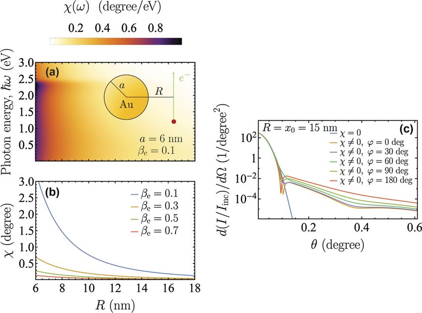
the resulting electron angular distribution calculated from equation (50) in figure 3(c) (χ = 0 curves) for a
gold nanosphere of radius a = 6 nm ( λe ) and an electron beam of velocity v = 0.1 c, width σ R = 5 nm,
and impact parameter x0 = 15 nm relative to the particle center. We further compare the scattering pattern
with the one obtained in the absence of the nanoparticle (i.e., setting χ = 0), which takes the analytical
form (also assuming a λe )
dI 2k2 σ 2 cos2 θ
= Iinc 0 R exp −2k20 σR2 sin2 θ . (51)
dΩ π
15You can also read