Conditional simulation of surface rainfall fields using modified phase annealing
←
→
Page content transcription
If your browser does not render page correctly, please read the page content below
Hydrol. Earth Syst. Sci., 24, 2287–2301, 2020
https://doi.org/10.5194/hess-24-2287-2020
© Author(s) 2020. This work is distributed under
the Creative Commons Attribution 4.0 License.

Conditional simulation of surface rainfall
fields using modified phase annealing
Jieru Yan1 , András Bárdossy2 , Sebastian Hörning3 , and Tao Tao1
1 College of Environmental Science and Engineering, Tongji University, Shanghai, China
2 Instituteof Modeling Hydraulic and Environmental Systems, Department of Hydrology and Geohydrology,
University of Stuttgart, Stuttgart, Germany
3 Centre for Natural Gas, Faculty of Engineering, Architecture and Information Technology,

the University of Queensland, Brisbane, Australia

Correspondence: Jieru Yan (yanjieru1988@163.com)

Received: 5 January 2020 – Discussion started: 10 January 2020
Revised: 17 March 2020 – Accepted: 7 April 2020 – Published: 8 May 2020

Abstract. The accuracy of quantitative precipitation estima-       1   Introduction
tion (QPE) over a given region and period is of vital impor-
tance across multiple domains and disciplines. However, due        Quantitative precipitation estimation (QPE) over a given re-
to the intricate temporospatial variability and the intermittent   gion and period is of vital importance across multiple do-
nature of precipitation, it is challenging to obtain QPE with      mains and disciplines. Yet the intricate temporospatial vari-
adequate accuracy. This paper aims to simulate rainfall fields     ability, together with the intermittent nature of precipita-
while honoring both the local constraints imposed by the           tion in both space and time, has hampered the accuracy
point-wise rain gauge observations and the global constraints      of QPE (Kumar and Foufoula-Georgiou, 1994; Emmanuel
imposed by the field measurements obtained from weather            et al., 2012; Cristiano et al., 2017).
radar. The conditional simulation method employed in this             The point-wise observations of precipitation measured by
study is modified phase annealing (PA), which is practically       rain gauges are accurate but only available at limited loca-
an evolution from the traditional simulated annealing (SA).        tions. Meanwhile, precipitation-related measurements pro-
Yet unlike SA, which implements perturbations in the spatial       duced by meteorological radars have become standard out-
field, PA implements perturbations in Fourier space, mak-          puts of weather offices in many places in the world. How-
ing it superior to SA in many respects. PA is developed in         ever, the problem with radar-based QPE is the nonguaran-
two ways. First, taking advantage of the global characteristic     teed accuracy, which could be impaired by various sources
of PA, the method is only used to deal with global constraints,    of errors, such as static/dynamic clutter, signal attenuation,
and the local ones are handed over to residual kriging. Sec-       anomalous propagation of the radar beam, uncertainty in the
ond, except for the system temperature, the number of per-         Z–R relationship, etc. (see Doviak and Zrnić, 1993; Collier,
turbed phases is also annealed during the simulation process,      1999; Fabry, 2015, for details). Despite the various sources
making the influence of the perturbation more global at ini-       of error, weather radar has been widely acknowledged as a
tial phases and decreasing the global impact of the perturba-      valid indicator of precipitation patterns (e.g., Mendez Anto-
tion gradually as the number of perturbed phases decreases.        nio et al., 2009; Fabry, 2015). Considering the pros and cons
The proposed method is used to simulate the rainfall field         of the two most usual sources of precipitation information,
for a 30 min event using different scenarios: with and with-       the QPE obtained by merging the point-wise rain gauge ob-
out integrating the uncertainty of the radar-indicated rainfall    servations and the radar-indicated precipitation pattern has
pattern and with different objective functions.                    become a research problem in both meteorology and hydrol-
                                                                   ogy (Hasan et al., 2016; Yan and Bárdossy, 2019).

Published by Copernicus Publications on behalf of the European Geosciences Union.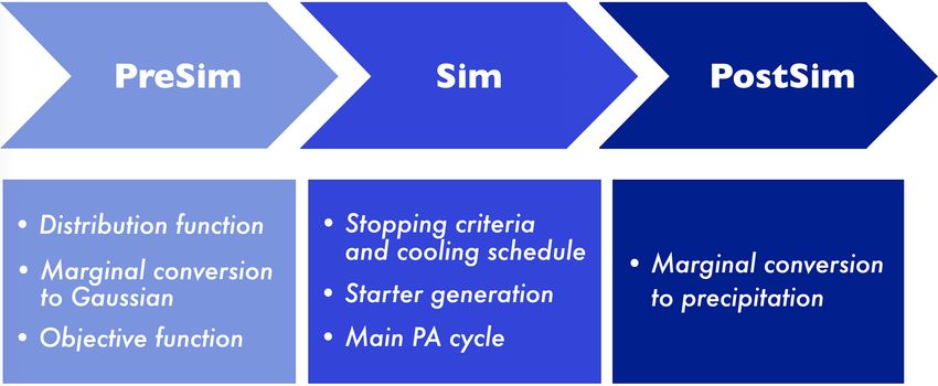
2288                          J. Yan et al.: Conditional simulation of surface rainfall fields using modified phase annealing

   In the context of merging radar and rain gauge data, we
consider two types of constraints: the local constraints im-
posed by the point-wise rain gauge observations and the
global constraints imposed by the field measurement from
weather radar. This paper focuses on simulating surface rain-
fall fields conditioned on the two types of constraints. There
exists a variety of geostatistical methods aiming to simulate
conditional Gaussian fields with a given covariance function,
such as turning bands simulation, LU-decomposition-based
methods, sequential Gaussian simulation, etc. (see Deutsch            Figure 1. Flowchart of the procedure to simulate surface rainfall
and Journel, 1998; Chilès and Delfiner, 2012; Lantuéjoul,             fields using the algorithm of PA.
2013, for details). The common goal of these methods is to
ensure that the simulated realizations comply with the ad-
ditional information available (Lauzon and Marcotte, 2019).           could be considered in the simulation, and the inability of PA
The additional information could be observed values of the            to handle the local constraints can be utilized in turn. How-
simulated targets, measurements that are related linearly or          ever, in the general case, the local constraints can only be
nonlinearly to the simulated targets, third- or higher-order          approximated by PA.
statistics (Guthke and Bárdossy, 2017; Bárdossy and Hörn-                Respecting the fact that the specialty of PA is the treat-
ing, 2017), etc.                                                      ment of the global constraints, we separate the global from
   The conditional simulation method used in this work is             the local. In particular, PA is only used to handle the global
phase annealing (PA). It was first proposed in Hörning and            constraints, and local ones are handled separately by residual
Bárdossy (2018) and is essentially a product of the general-          kriging at each iteration. As an extension of PA, except for
purpose metaheuristics method of simulated annealing (SA)             annealing the system temperature, the number of perturbed
(Kirkpatrick et al., 1983; Geman and Geman, 1984; Deutsch,            phases is annealed in parallel to render the algorithm to work
1992; Deutsch and Journel, 1994). It utilizes the sophisti-           more globally at initial phases of the simulation. The global
cated optimization scheme of SA in the search for the global          impact of the perturbation is weakened as the number of per-
optimum. Yet compared to SA, the distinction or evolvement            turbed phases decreases.
of PA lies in the fact that the perturbation, or swapping in             This paper is divided into six sections. After the general
the nomenclature of SA, is implemented in Fourier space.              introduction, the methodology of PA is introduced in Sect. 2,
Or, to be more exact, the perturbation is implemented on the          including three stages: presimulation, simulation, and post-
phase component of the Fourier transform, while the power             simulation. Section 3 provides two options to integrate the
spectrum is preserved such that the spatial covariance is in-         uncertainty of the radar-indicated rainfall pattern into the
variant at all iterations according to the well-known Wiener–         simulation. Section 4 introduces the study domain and the
Khinchin theorem (Wiener, 1930; Khintchine, 1934). Com-               two types of data used in this study. In Sect. 5, the proposed
pared to SA, PA alleviates the singularity problem, namely            algorithm is used to simulate the rainfall field for a 30 min
the undesired discontinuities or poor embedding of the con-           event, where different simulation scenarios are applied. Sec-
ditional points within the neighborhood (Hörning and Bár-             tion 6 ends this paper with conclusions.
dossy, 2018), and in general, PA has a much higher conver-
gence rate compared to SA.
   A remarkable feature of PA is that it is a global method:          2     Methodology
any perturbation imposed on the phase component is re-
flected in the entire field. Yet admittedly, if the perturbation is   Figure 1 summarizes the procedure of simulating surface
implemented at lower frequencies where the corresponding              rainfall fields using the algorithm of PA, including three
wave lengths are relatively large, the impact is more global          stages: presimulation (PreSim), simulation (Sim), and post-
and vice versa. The global characteristic of PA makes it a            simulation (PostSim). Each stage and the corresponding sub-
valuable methodology for global constraints. However, PA is           stages are described in the following subsections in the same
found to be insufficient in the treatment of local constraints        sequence as shown in the flowchart.
(Hörning and Bárdossy, 2018). Note that by local constraints,
we refer primarily to point equality constraints when the total       2.1     Presimulation
number of constraints is far less than that of the grid points.
In the algorithm of PA, the local constraints are normally en-        2.1.1    Distribution function of surface rainfall
sured by inserting a component measuring the dissimilarity
between the simulated and the target values. On the other             PA is embedded in Gaussian space. The direct output of
hand, one could argue that if the information on the measure-         the PA algorithm is a spatial field whose marginal distribu-
ment error is explicitly known, then this piece of information        tion function is standard normal; hence the distribution func-

Hydrol. Earth Syst. Sci., 24, 2287–2301, 2020                                       www.hydrol-earth-syst-sci.net/24/2287/2020/
J. Yan et al.: Conditional simulation of surface rainfall fields using modified phase annealing                                2289

tion of surface rainfall is essential to transform the simulated            where the only parameter λ of the exponential distribu-
Gaussian fields into rainfall fields of interest.                           tion is determined from the last pair (rK , uK ):
   The scenario is as follows: based on K rain gauge obser-
vations and a regular grid of radar quantiles (representing the             λ = − ln (1 − uK ) /rK .                             (4)
spatial pattern of the rainfall field), the distribution function
of surface rainfall is generated. The procedure was first in-          It is recommended that the methodology described above
troduced in Yan and Bárdossy (2019), and we specify the             is used to estimate the distribution function of accumulated
modified version here.                                              rainfall, not rain intensity, because it is built on the assump-
                                                                    tion that rain gauge observations can represent the ground
  a. For all rain gauge observations rk , the collocated quan-
                                                                    truth. Yet in general, rain gauges are considered to be poor
     tiles in the radar quantile map U are determined and
                                                                    in capturing the instantaneous rain intensity, while the mea-
     denoted as uk . The two datasets are then sorted in as-
                                                                    surement error diminishes rapidly as the integration time in-
     cending order, i.e., r1 ≤ · · · ≤ rK and u1 ≤ · · · ≤ uK .
                                                                    creases (Fabry, 2015).
  b. Set the spatial intermittency u0 , i.e., the quantile cor-        As we only use the radar-indicated spatial ranks, i.e., the
     responding to zero precipitation. u0 is estimated as the       scaled radar map following a uniform distribution in [0, 1],
     ratio of the number of zero-valued pixels to the total         there is no requirement for the accuracy of the Z–R rela-
     number of pixels in the domain of interest. If the small       tion given the monotonic relationship of the two quantities.
     quantiles of the field are properly sampled by the rain        One could use a Z–R relation at hand to transform radar re-
     gauges, one could use the smallest sampled quantile u1         flectivity into rain intensity and then make the accumulation.
     to estimate u0 :                                               Nevertheless, a normal quality control for radar data, as de-
                                                                    scribed in Sect. 4, is necessary to maintain the accuracy of
                                                                    radar-indicated spatial ranks.

              u1      if r1 = 0
     u0 =                                                   (1)
              u1 /2 otherwise,
                                                                    2.1.2     Marginal conversion to Gaussian
     where r1 is the smallest gauge observation correspond-
     ing to u1 . As an alternative, if the small quantiles of       As PA is embedded in Gaussian space, all the constraints,
     the field are not properly sampled by the rain gauges,         including the point equality targets rk (mm) imposed by rain
     we propose to estimate u0 from the original radar dis-         gauges and the quantile map U (–) imposed by weather radar,
     plays in dBZ, namely a series of instantaneous maps of         are converted to a standard normal marginal distribution by
     radar reflectivity within the relevant accumulation time.
     A zero-valued pixel is defined when the maximum of             zk = 8−1 (G (rk )) for k = 1, · · ·, K                       (5)
     the collocated pixel values of these maps is smaller than       ∗         −1
                                                                    Z =8            (U ),                                        (6)
     a given threshold (say 20 dBZ).
                                                                    where 8−1 is the inverse of the cumulative standard normal
  c. Let G(r) denote the distribution function of surface           distribution function and G is the distribution function of sur-
     rainfall to be estimated. A linear interpolation is applied    face rainfall obtained according to the procedure described in
     for rainfall values of less than the maximum recorded          Sect. 2.1.1.
     gauge observations, i.e., r ≤ rK :
                                                                    2.1.3     Objective function
              uk − uk−1
     G(r) =             (r − rk−1 ) + uk−1 ,                 (2)
              rk − rk−1                                             We impose two kinds of constraints: local and global. As has
                                                                    been explained in the introduction, PA is a powerful method
     with rk−1 , rk being the two nearest neighbors of r            for handling global constraints. In order not to interfere with
     (rk−1 ≤ r ≤ rk ) and uk−1 , uk being the quantiles corre-      the logic behind PA and to fulfill the point equality con-
     sponding to rk−1 , rk , respectively.                          straints (local constraints) exactly, residual kriging is imple-
                                                                    mented at each iteration to obtain the observed values at rain
  d. Extrapolate rainfall values r > rK . A modification is
                                                                    gauge locations. Thus the objective function only needs to
     made here: the minimum of exponential and linear ex-
                                                                    measure the fulfillment of the global constraints.
     trapolation is used as the result, as expressed in Eq. (3).
                                                                       We impose two global constraints: field pattern and direc-
     We have learned from practice that the exponential ex-
                                                                    tional asymmetry. Note that both constraints are evaluated
     trapolation tends to overestimate the rainfall extremes,
                                                                    from the simulated Gaussian field and are compared with the
     so a linear component is used to restrict the extrapola-
                                                                    radar-based Gaussian field Z ∗ , as obtained in Eq. (6). We
     tion result.
                                                                    term Z ∗ the reference field hereafter.
                                                                       The first global constraint, field pattern, requires the sim-

                              uK − uK−1
     G(r) = min 1 − e−λr ,                 (r − rK ) + uK , (3)     ulated field to be similar to the reference field. The similarity
                              rK − rK−1

www.hydrol-earth-syst-sci.net/24/2287/2020/                                           Hydrol. Earth Syst. Sci., 24, 2287–2301, 2020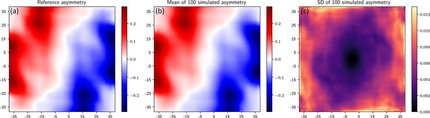
2290                         J. Yan et al.: Conditional simulation of surface rainfall fields using modified phase annealing

of the two fields is quantified by the Pearson correlation co-     threshold of the initial objective function value, and so forth.
efficient:                                                         One could use one criterion or combine several.
           cov (Z, Z ∗ )                                              As for the cooling schedule, the system temperature of
ρZ,Z ∗ =                 .                                  (7)    PA decreases according to the cooling schedule as the opti-
              σZ σZ∗
                                                                   mization process develops: the lower the system temperature,
In the ideal case, ρZ,Z ∗ equals 1, and we use the difference      the less likely a bad perturbation is accepted. A bad perturba-
(1 − ρZ,Z ∗ ) to measure the distance from the ideal.              tion occurs when the perturbation does not decrease the ob-
   The second global constraint is directional asymmetry, as       jective function value. A reasonable cooling schedule is ca-
given by                                                           pable of preventing the optimization from being trapped pre-
                                                                   maturely at a local minimum. Yet one should be aware that
               1     X                          3
                                                                   there is always a compromise between the statistical guaran-
[A(h)]Z =                  8 (Z (xi )) − 8 Z xj      ,      (8)
             N (h) x −x ≈h                                         tee of the convergence and the computational cost: the slower
                     i   j
                                                                   the temperature decreases, the higher the probability of the
where [A(h)]Z (abbreviated as AZ hereafter) is the asymme-         convergence. However, cooling slowly also means more iter-
try function evaluated from the simulated Gaussian field Z,        ations and therefore higher computational costs.
N(h) is the number of pairs fulfilling xi − xj ≈ h, and 8 is          Comparative studies of the performance of SA using the
the cumulative standard normal distribution function. Direc-       most important cooling schedules, i.e., multiplicative mono-
tional asymmetry was first introduced in Bárdossy and Hörn-        tonic, additive monotonic, and nonmonotonic adaptive cool-
ing (2017) and Hörning and Bárdossy (2018). It is a third-         ing, have been made by, e.g., Nourani and Andresen (1998),
order statistic, and the physical phenomenon revealed by           Martín and Sierra (2020), and others. The results show that
this statistic could be significant for advection-dominant pro-    annealing works properly when the cooling curve has a mod-
cesses, such as storms. We use the entire field to compute the     erate slope at the initial and central stages of the process and
directional asymmetry function and compare the simulated           tends to have a softer slope at the final stage. Many cooling
one with the reference asymmetry function, i.e., the direc-        schedules satisfy these conditions. As PA utilizes the opti-
tional asymmetry function evaluated from the reference field,      mization strategy of SA, the rules also apply for PA. Our
abbreviated as AZ ∗ . There exist multiple choices to define the   choice of the cooling schedule is the multiplicative mono-
distance of the two asymmetry functions, and we have used          tonic one.
the L∞ norm kAZ − AZ ∗ kL∞ .                                          Specifically, we search for two parameters – the initial
   Different schemes could be used to combine the two com-         temperature T0 and the final temperature Tmin – by decreas-
ponents, linear or nonlinear, and we have chosen the maxi-         ing the temperature exponentially and discretely. At each
mum of the two components. Finally, the objective function         fixed temperature, N perturbations, say 1000, are imple-
we have used to quantify the fulfillment of the two global         mented, and the corresponding acceptance rate and improve-
constraints is expressed as                                        ment rate are computed. Acceptance means the perturbation
                                                                 is accepted by the system, and the system state is updated ir-
O(Z) = max 1 − ρZ,Z ∗ , (w/Ascal ) · kAZ − AZ ∗ kL∞ , (9)
                                                                   respective of whether the perturbation brings improvement to
where w is the relative weight of the component directional        the system, while improvement means the perturbation does
asymmetry, and Ascal , as expressed in Eq. (10), is the scaling    decrease the objective function value. In short, a perturba-
factor that scales the L∞ norm of the difference of the two        tion that brings improvement must be an accepted perturba-
asymmetry functions between 0 and 1.                               tion, yet an accepted perturbation does not necessarily bring
                                                                   improvement to the system. We refer to the experiment as a
Ascal = kAZ ∗ kL∞                                          (10)    temperature cycle, where N perturbations are implemented,
                                                                   and the two mentioned rates are computed at a fixed temper-
It is worth mentioning that the proposed methodology is flex-
                                                                   ature.
ible, and any global statistic could be used to constrain the
                                                                      T0 is first set by starting a temperature cycle with an initial
simulated fields. One could even combine several statistics
                                                                   guess of T0 . If the acceptance rate is lower than the prede-
in the objective function.
                                                                   fined limit, say 98 %, then the temperature is increased and
2.2     Simulation                                                 vice versa. The goal is to find a T0 with a relatively high
                                                                   acceptance rate. Then, Tmin is set by decreasing T0 exponen-
2.2.1    Stopping criteria and cooling schedule                    tially until the predefined stopping criterion is met. It is clear
                                                                   in our case that if more iterations are implemented, better re-
There are many choices of stopping criteria for an optimiza-       alizations (realizations with lower objective function values)
tion algorithm, such as (a) the total number of iterations,        could be produced, yet it is again a compromise between a
(b) the predefined value of the objective function, (c) the rate   satisfactory destination and the computational cost.
of decrease of the objective function, (d) the number of con-         We note that from the determination of T0 , the total
tinuous iterations without improvement, (e) the predefined         number of temperature cycles m (to anneal T0 to Tmin ) is

Hydrol. Earth Syst. Sci., 24, 2287–2301, 2020                                    www.hydrol-earth-syst-sci.net/24/2287/2020/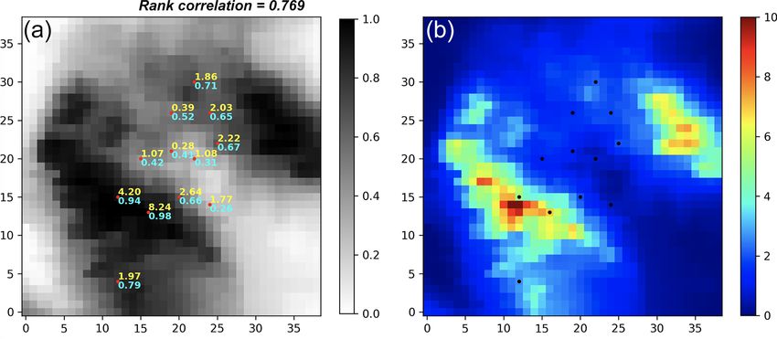
J. Yan et al.: Conditional simulation of surface rainfall fields using modified phase annealing                                           2291

recorded. Thus the total number of perturbations is estimated           2.2.3     Main PA cycle
as L = mN . A continuous cooling schedule is then computed
from T0 , Tmin , and L. The temperature at Iteration l is com-          The starting point of PA is a Gaussian random field ZK with
puted as                                                                the prescribed spatial covariance as described in Sect. 2.2.2.
                                                                        A little modification in our case is that the values at the obser-
Tl = T0 · αTl for l = 0, · · ·, L − 1,                          (11)    vational locations are fixed by residual kriging, as indicated
                                                                        by the subscript K. In particular, the procedure of residual
where αT is the attenuation factor of the system temperature,           kriging is explained in the following (Step 6). The procedure
given as                                                                of the PA algorithm applied in this paper is specified as fol-
                                                                    lows:
               Tmin
αT = exp ln            /(L − 1) .                        (12)
                 T0                                                       1. The discrete Fourier transform (DFT) of ZK is com-
                                                                             puted as
   In parallel with the temperature annealing we also anneal
the number of phases being perturbed in Fourier space, start-                   ZK = F{ZK }.                                               (15)
ing with a relatively large number N0 (say 5 % to 20 % of
the total number of valid Fourier phases) and decreasing all              2. The system temperature Tl and the number of perturbed
the way down to 1. The number of phases to be perturbed at                   phases Nl at Iteration l are computed by Eqs. (11)
Iteration l is computed by                                                   and (13).
            l                                                             3. Nl vectors (un , vn ) are generated, where n = 0, · · ·, Nl −
Nl = N0 · α N for l = 0, · · ·, L − 1,                          (13)
                                                                             1. un , vn are randomly drawn from the two discrete
where αN is the attenuation factor with respect to the number                uniform distributions [1, · · ·, U 0 ] and [1, · · ·, V 0 ], respec-
of perturbed Fourier phases. It is computed as                               tively, where U 0 , V 0 are the highest frequencies con-
                                                                             sidered for perturbation in the x and y directions, re-
αN = exp (− ln (N0 ) /(L − 1)) .                                (14)         spectively. Note that zero frequencies in both directions
                                                                             should be excluded from the perturbation. One could
   The logic behind annealing the number of perturbed                        use the entire frequency range or select a subarea to im-
phases is to render the perturbation to have a more global                   pose the perturbation.
impact initially when the distance from the destination is rel-
atively large and to decrease the impact of the perturbation              4. Nl phases θn are randomly drawn from the uniform dis-
gradually as the optimization process develops.                              tribution [−π , π).

2.2.2   Starter generation                                                5. The Fourier coefficients at the selected loca-
                                                                             tions (un , vn ) and the corresponding symmetrical
PA requires a starting Gaussian random field with the pre-                   locations are expressed as
scribed spatial covariance, abbreviated as starter. Various
methods could be used to generate such a random field,                          ZK [un , vn ] = an + j bn                                  (16)
e.g., fast Fourier transformation for regular grids (Wood and                   ZK [U − un , V − vn ] = an − j bn ,                        (17)
Chan, 1994; Wood, 1995; Ravalec et al., 2000), turning bands
simulation (Journel, 1974), or the Cholesky transformation                      where U , V are the number of grid points in x and y di-
of the covariance matrix. Considering the fact that the gauge                   rections, respectively, and are also the highest frequen-
observations used in this work cannot provide enough infor-                     cies in both directions. These coefficients are then up-
mation to derive the spatial covariance, the radar-based Gaus-                  dated in terms of the Fourier phases using θn , while the
sian field, i.e., the reference field Z ∗ , is used instead to derive           corresponding amplitudes remain unchanged:
the covariance.                                                                                 q
   It should be noted that if a fast Fourier transforma-                        ZK [un , vn ] ← an2 + bn2 · (cos (θn ) + j sin (θ )) (18)
tion (FFT) is used to generate the starter, the inherent peri-                                            q
odic property of the FFT should be treated with care. Specif-                   ZK [U − un , V − vn ] ← an2 + bn2
ically, the simulation should be embedded in a larger do-                                              · (cos (θn ) − j sin (θn )) .       (19)
main. The original domain is enlarged in all directions by
a finite range, i.e., the range bringing the covariance func-                   The perturbed Fourier transform is denoted as Z̃. The
tion from the maximum to approaching zero. If covariance                        corresponding perturbed spatial random field is ob-
models with asymptotic ranges (e.g., exponential, Matérn,                       tained by the inverse DFT:
and Gaussian covariances) are employed, the extension in
domain size could be significant (Chilès and Delfiner, 2012).                   Z̃ = F −1 {Z̃}.                                            (20)

www.hydrol-earth-syst-sci.net/24/2287/2020/                                             Hydrol. Earth Syst. Sci., 24, 2287–2301, 2020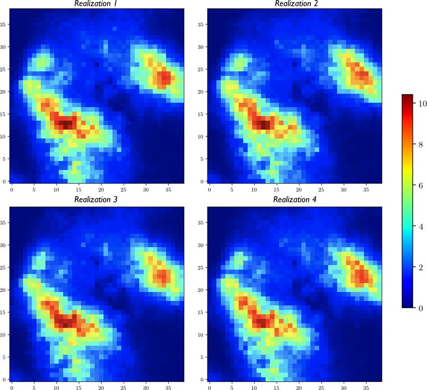
2292 J. Yan et al.: Conditional simulation of surface rainfall fields using modified phase annealing
6. Due to the perturbation, Z̃ no longer satisfies the The conflict of the two could be partially explained by
point equality constraints (note the removal of the sub- the fact that weather radar measures at some distance above
script K). Thus kriging is applied for the residuals the ground (a few hundred to more than a thousand meters
zk − Z̃(xk ), where zk represents the point equality con- aloft). It is therefore reasonable to suspect the correctness
straints defined in Eq. (5). The results of kriging r are of comparing the ground-based rain gauge observations with
superimposed on Z̃: the collocated radar data by assuming the vertical descent of
the hydrometeors. In fact, hydrometeors are very likely to be
Z̃K = Z̃ + r. (21) laterally advected during their descent by wind, which occurs
quite frequently concurrently with precipitation. To take the
As kriging is a geostatistical method that depends only
possible wind-induced displacement into account, the proce-
on the configuration of the data points, the weight ma-
dure described in Yan and Bárdossy (2019) is adopted. Here
trix of individual grid points does not change with iter-
we recall the procedure briefly in three steps.
ations. One needs to compute the weight matrices for
all the grid points only once. Thus residual kriging is 1. A rank correlation matrix ρ Sij is generated by first shift-
cheap to use and causes almost no additional computa- ing the original radar quantile map U with all the vec-
tional cost. tors defined by a regular grid hij , i.e., locations of all
the grid cells in hij , and then calculating the rank cor-
7. Z̃K is then subject to the objective function defined relation between gauge observations and the collocated
in Eq. (9). If O(Z̃K ) < O(ZK ), the perturbation is ac- radar quantiles in the shifted map. Note that the radar
cepted. Otherwise, the perturbation is accepted with the quantile map shifted by vector hij (a certain grid cell in
probability hij ) is denoted as Uij .
Both hij and ρ Sij have the same spatial resolution as U .
O (ZK ) − O Z̃K
P = exp . (22) The center of hij is (0, 0), with the corresponding entry
Tl in ρ Sij denoted as ρ00
S , meaning that zero shift is imposed
on U . The farther a grid cell is from the center, the larger
8. If the perturbation is accepted, the system state is up- the shift imposed on U is. One should limit the number
dated; namely ZK , ZK and O(ZK ) are replaced by Z̃K , of grid cells in hij depending on the radar measurement
Z̃K , and O(Z̃K ), respectively. height.
9. If the stopping criterion is met, the optimization is 2. A probability matrix Pij is generated from the rank cor-
stopped and ZK is a realization in Gaussian space, sat- relation matrix ρ Sij :
isfying the predefined optimization criterion. Otherwise
for ρijS ≤ ρ00
S
(
go to Step 2. 0
Pij = (24)
H ρijS otherwise,
2.3 Postsimulation
where H is a monotonic function, such as power func-
The Gaussian field ZK is transformed into a rainfall field by tion, exponential function, or logarithmic function. The
first derivative (dH /dx) matters as a large dH /dx
R = G−1 (8 (ZK )) , (23) means that more weights are assigned to those displace-
where 8 is the cumulative standard normal distribution func- ment vectors (or shifted fields) that produce a higher-
tion, and G−1 is the inverse of the distribution function of rank correlation. Our choice of function H is simply
surface rainfall, as obtained in Sect. 2.1.1. The resultant R is H (x) = x 2 .
a realization of the surface rainfall field. 3. The probability matrix Pij is scaled to ensure that the
sum of all entries equals 1:
3 Uncertainty of radar-indicated rainfall pattern Pij
Pij = PP . (25)
Pij
The two datasets – gauge observations rk and the collocated i j
radar quantiles uk – are supposed to have the same rankings;
Pij quantifies the uncertainty of the radar-indicated
namely large gauge observations should correspond to large
rainfall pattern by giving the probability of individ-
quantiles and vice versa. Yet it is not always the case, which
ual shifted quantile fields in analogy with a probability
reveals the conflict of radar and gauge data. To quantify the
mass function. The logic behind it is that only those dis-
conflict, we employ the (Spearman’s) rank correlation ρ S that
placement vectors that increase the accordance of radar
measures the monotonic relationship of two variables: the
and gauge data are accepted and given strong probabil-
closer ρ S is to 1, the more accordance (or less conflict) of
ity.
radar and gauge data.
Hydrol. Earth Syst. Sci., 24, 2287–2301, 2020 www.hydrol-earth-syst-sci.net/24/2287/2020/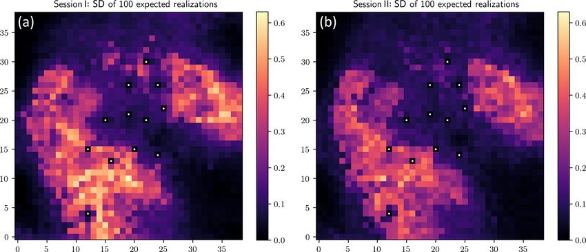
J. Yan et al.: Conditional simulation of surface rainfall fields using modified phase annealing 2293
The method described above is built on the assumption
that the entire field is displaced by a single vector. The extent
of the domain in this work is 19 km × 19 km (see Sect. 4 for
details), and the selection of the extent is limited by the gauge
data availability. With this spatial extent, we could quite often
find dozens of displacement vectors that bring up the concor-
dance of radar and gauge data. If gauge data accessibility is
not the limiting factor, one could enlarge the extent (say to
40 km × 40 km), provided that the resultant probability ma-
trix has some pattern (not a random field).
There are two options to integrate the uncertainty of the
radar-indicated rainfall pattern, i.e., the information carried
by the probability matrix Pij , into the simulation.
Option 1: the expectation of the shifted quantile fields is
computed using the probability matrix, and then the corre-
sponding Gaussian field is computed, as given in Eq. (26).
The result is used as the reference field when applying the
PA algorithm.
!
XX
∗ −1
Z =8 Pij · Uij (26)
i j
Option 2: those (marginally converted) shifted quantile
fields 8−1 (U ij ) bearing a positive probability are considered
as reference fields, and the algorithm described in Sect. 2 is
applied independently for all these reference fields. The re-
Figure 2. The elevation map of Baden-Württemberg with the study
sults are multiple realizations of the surface rainfall field with
domain marked by the red square, the rain gauges marked by the
different references, denoted as R ij . The estimate of the sur- red dots, and the site of Radar Türkheim marked by the red star.
face rainfall field (with the uncertainty of the radar-indicated
rainfall pattern integrated) is obtained as the expectation of
these realizations: Heistermann, 2016), (3) reprojection from polar to Carte-
XX
R= Pij · Rij . (27) sian coordinates, and (4) clipping of the square data for the
i j study domain. All these quality control steps are operated in
the wradlib environment, an open-source library for weather
Both options are capable of producing estimates of the sur-
radar data processing (Heistermann et al., 2013).
face rainfall field with the uncertainty of the radar-indicated
rainfall pattern integrated, yet the results are distinct, as pre-
sented in Sect. 5.
5 Application
4 Study domain and data We selected a 30 min event to apply the algorithm of PA. The
event was selected not only due to the relatively prominent
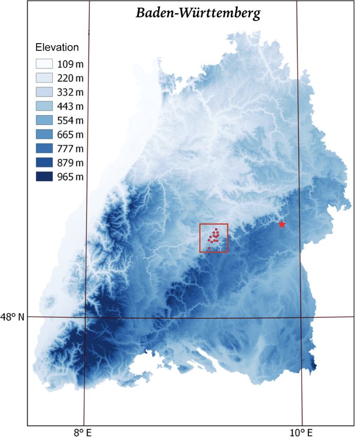
The study domain is located in Baden-Württemberg, in the rain intensity reflected by the rain gauge data, but more im-
southwest of Germany. As shown in Fig. 2, it is a square do- portantly because the event was properly captured by a few
main with a side length of 19 km. The domain is discretized rain gauges unevenly distributed in the domain of interest, as
to a 39 × 39 grid with a spatial resolution of 500 m × 500 m. shown by the red dots in Fig. 3a. From the figure, it can be
A gauge network consisting of 12 pluviometers is available clearly seen that the sampled quantiles (indicated by the text
within the domain, as denoted by the red dots in Fig. 2. in cyan) cover the entire range [0, 1]: not only the small or
The radar data used in this study are the raw data with large ones, but the sampled quantiles as well are more or less
5 min temporal resolution, measured by Radar Türkheim, evenly distributed. One might have noticed that the smallest
a C-band radar operated by the German Weather Ser- sampled quantile is 0.53. Yet in this case, u0 = 0.26 (the spa-
vice (DWD). Radar Türkheim is located about 45 km from tial intermittency) and the quantile value 0.53 correspond to
the domain center, as denoted by the red star in Fig. 2. the rainfall value 0.28 mm after the re-ordering.
The raw data are subject to a processing chain consisting of The conflict of radar and gauge data is obviously reflected
(1) clutter removal (Gabella and Notarpietro, 2002), (2) at- in Fig. 3 (left), for example, the collocation of 4.20 mm rain-
tenuation correlation (Krämer and Verworn, 2008; Jacobi and fall with the quantile 0.99 in contrast with the collocation of
www.hydrol-earth-syst-sci.net/24/2287/2020/ Hydrol. Earth Syst. Sci., 24, 2287–2301, 2020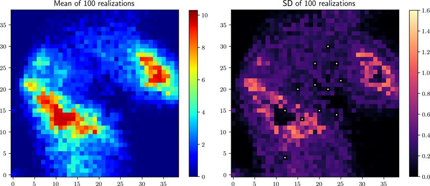
2294 J. Yan et al.: Conditional simulation of surface rainfall fields using modified phase annealing
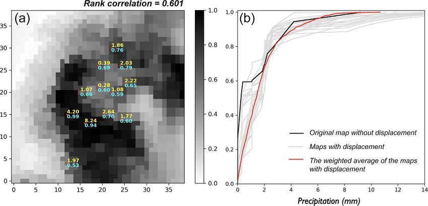
Figure 3. (a) Original radar quantile map (–) for the 30 min event (4 May 2017, 13:20–13:50 LT), with the rain gauge observations (mm)
labeled in yellow and the collocated radar quantiles labeled in cyan. (b) Distribution functions of surface rainfall. Black: original radar map
without displacement; gray: radar maps with displacement; red: the weighted average of the radar maps with displacement.
8.24 mm rainfall with the quantile 0.94. The rank correlation hence, with a denser network of rain gauges, a good perfor-
of the gauge observations and the collocated radar quantiles mance of the methodology is more likely guaranteed.
is 0.601, as labeled in the title of the figure. The distribution We open up two simulation sessions, depending on the dif-
function of the surface rainfall field based on the two original ferent objective functions used when applying the PA algo-
datasets is shown by the black line in Fig. 3b. rithm. In Session I, the objective function contains only the
However, using the algorithm described in Sect. 3 to evalu- component field pattern O(Z) = 1−ρZ,Z ∗ . In Session II, the
ate the uncertainty of the radar-indicated rainfall pattern, one component directional asymmetry comes into play, and the
can obtain multiple distribution functions of surface rainfall, objective function expressed in Eq. (9) is employed, where
as shown by the gray lines in Fig. 3b. Note that only the dis- the relative weight of the component directional asymme-
tribution functions associated with those shifted fields pos- try w equals 0.5. Technically, for both simulation sessions,
sessing a positive probability (as indicated by the probability the optimization process stops when the objective function
matrix) are shown in the figure. falls below 0.05.
With these distribution functions, one can transform the
corresponding shifted quantile fields into rainfall fields, and 5.1 Simulation Session I
with the probability matrix, the expectation of these rainfall
fields can be computed, as shown in Fig. 4b. Also with the We present an evolution in terms of the simulation strat-
probability matrix, one can compute the expectation of the egy where the algorithm of PA is applied differently in three
shifted quantile fields, as shown in Fig. 4a. From the expected stages:
quantile map, a tangible improvement in terms of the concor-
dance of radar and gauge data is observed: the rank correla- 1. using the original quantile map as the reference
tion increases from 0.601 to 0.769, as labeled in the title of
Figs. 3 and 4. 2. using the expected quantile map as the reference, i.e.,
It is noteworthy that the data configuration used in this integrating the uncertainty of the radar-indicated rainfall
work is not good enough to maximize the performance of the pattern via Option 1 in Sect. 3
proposed methodology as the distribution of the rain gauges
3. simulating independently using those shifted quantile
is relatively centered. Thus we have to select events whose
maps with a positive probability as the reference and
storm center is relatively centered according to the radar
computing the expectation, i.e., integrating the uncer-
map. To enlarge the applicability, it is recommended that rain
tainty of the radar-indicated rainfall pattern via Option 2
gauges are uniformly distributed in the domain of interest. In
in Sect. 3.
addition to the distribution of the rain gauges, as shown in the
following, the effect of conditioning on gauge observations is Stage 1 (simulating rainfall fields using the original quan-
local (in consistency with the terminology local constraints); tile map as the reference) means the uncertainty of the radar-
indicated rainfall pattern is not integrated. Figure 5 shows the
Hydrol. Earth Syst. Sci., 24, 2287–2301, 2020 www.hydrol-earth-syst-sci.net/24/2287/2020/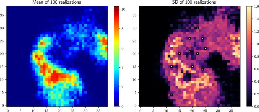
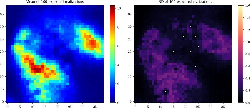
J. Yan et al.: Conditional simulation of surface rainfall fields using modified phase annealing                                       2295

Figure 4. (a) The expected quantile map (–), with the rain gauge observations (mm) labeled in yellow and the collocated radar quantiles
labeled in cyan. (b) The expected rainfall field (mm).

Figure 5. Stage 1 results: mean and standard deviation of 100 realizations (mm), obtained using the original quantile map as the reference.

mean of 100 such realizations on the left and the correspond-           reduced estimation uncertainty by integrating the uncertainty
ing standard deviation map on the right. The standard devia-            of the radar-indicated rainfall pattern.
tion map reflects the variability of different realizations, and           Stage 3 involves a simulation strategy that is slightly more
the pixel values, collocated with the rain gauges, are zeros, as        complicated than before. The simulation is applied indepen-
marked by the white points in Fig. 5 (right), which shows the           dently using the shifted quantile map associated with a pos-
fulfillment of the point equality constraints and the local ef-         itive probability as the reference, and the single simulation
fect of conditioning to the gauge observations. And this local          cycle is applied to all the components possessing a positive
effect is reflected in all the standard deviation maps shown in         probability. Finally, the expectation of these realizations is
the following.                                                          computed, termed the expected realization hereafter. Yet the
   Stage 2 (simulating rainfall fields using the expected quan-         computational cost to obtain such an expected realization is
tile map as the reference) integrates the uncertainty of the            much higher as multiple realizations are required to make up
radar-indicated rainfall pattern via Option 1, as described in          an expected realization (see Table 1 for details). Similarly,
Sect. 3. Similarly, the mean of 100 such realizations and the           the mean of 100 expected realizations and the correspond-
corresponding standard deviation map are shown in Fig. 6.               ing standard deviation map are shown in Fig. 7. Comparing
Comparing Figs. 5 and 6, one could observe the displace-                Figs. 6 and 7, the positions of the peak regions remain un-
ments of the peak regions in both the rainfall and the stan-            changed in both the rainfall and the standard deviation maps.
dard deviation maps. Compared to Fig. 5, a visible reduction            Yet compared to Fig. 6, the reduction in the standard devi-
in the standard deviation is observed in Fig. 6, showing the

www.hydrol-earth-syst-sci.net/24/2287/2020/                                            Hydrol. Earth Syst. Sci., 24, 2287–2301, 2020
2296                          J. Yan et al.: Conditional simulation of surface rainfall fields using modified phase annealing

Figure 6. Stage 2 results: mean and standard deviation of 100 realizations (mm), obtained using the expected quantile map as the reference.

Figure 7. Stage 3 results: mean and standard deviation of 100 expected realizations (mm).

ation is remarkable in Fig. 7, showing further reduction in                We still adopt the three-stage evolution when applying the
terms of the estimation uncertainty.                                    PA algorithm as in Simulation Session I. Differences be-
   In addition, the mean field and the standard deviation map           tween realizations from Session I and Session II do exist,
of the results from Stage 3 are much smoother compared to               but they are not that remarkable. Therefore, in the presenta-
the other alternatives shown previously. Figure 8 displays              tion of the results from Session II, we omit the results from
four randomly selected expected realizations to show the                Stages 1 and 2 and only display the results from Stage 3 in
similarity of different expected realizations and the smooth-           Figs. 9 and 10 (both panels on the right of each figure). The
ness of individual expected realizations.                               corresponding results from Session I are presented on the left
                                                                        just for the sake of comparison and identifying the effect of
5.2    Simulation Session II                                            adding the component asymmetry in the objective function.
                                                                        Comparing the two mean fields in Fig. 9, the distinction is in
In the previous session, the objective function only con-               the peak values: the two have similar estimates for the peak
tains the component field pattern. In this session, the com-            values of the large rain cell yet different estimates for those
ponent directional asymmetry (abbreviated as asymmetry                  of the small cell. As for the comparison of the standard de-
hereafter) comes into play in the objective function. It should         viation maps in Fig. 10, a slight reduction in the standard
be noted that the evaluation cost of the objective function in          deviation of Session II can be observed.
Session II is higher than that in Session I, and more time is              From the results shown in Figs. 9 and 10, the effect of
needed to generate a single realization if the same stopping            adding the component asymmetry in the objective function
criterion is used (see Table 1 for details).                            seems to be minor, which is due to the fact that the two com-

Hydrol. Earth Syst. Sci., 24, 2287–2301, 2020                                          www.hydrol-earth-syst-sci.net/24/2287/2020/
J. Yan et al.: Conditional simulation of surface rainfall fields using modified phase annealing 2297 Figure 8. Stage 3 results: four randomly selected expected realizations (mm). Figure 9. Mean of 100 expected realizations (mm) from Session I (a) and Session II (b). www.hydrol-earth-syst-sci.net/24/2287/2020/ Hydrol. Earth Syst. Sci., 24, 2287–2301, 2020
2298                          J. Yan et al.: Conditional simulation of surface rainfall fields using modified phase annealing

Figure 10. Standard deviation of 100 expected realizations (mm) from Session I (a) and Session II (b).

Figure 11. (a) Reference asymmetry function. (b, c) Mean and standard deviation of 100 simulated asymmetry functions. Unit: –.

ponents (field pattern and asymmetry) share a special rela-             havior of the field is assumed, the function value approaches
tionship: high similarity in terms of the pattern between the           zero.
reference and the simulated field suggests high similarity in              As shown in Fig. 11, the reference and the mean asym-
the asymmetry of the two as well. Yet, it does not work in              metry are barely distinguishable. The standard deviation
reverse.                                                                map, displayed on the right, reveals the small variability be-
   To show the capability of the proposed method in terms of            tween the simulated asymmetry functions. Note that the pre-
fulfilling the component asymmetry, the mean of 100 sim-                sented asymmetry functions are evaluated from realizations
ulated asymmetry functions is displayed in the middle in                of Stage 1. But a similar standard in terms of the fulfillment
Fig. 11 in comparison with the reference asymmetry func-                of the component asymmetry can be achieved by all the other
tion (the one evaluated from the reference field) on the left.          results from Session II.
As for the analysis of the asymmetry function: first, it is a              It is worth mentioning that a trick is used to reduce the
symmetrical function with respect to the origin (0, 0) (see the         computational cost substantially at a fairly low cost in terms
formula given in Eq. (8)); second, the value of each pixel is           of the estimation quality. In Sect. 3, when using multiple
obtained by (a) shifting the simulated field by the coordinate          shifted quantile fields to produce the expected realization,
of the pixel and then (b) evaluating Eq. (8) for the intersec-          one should be aware that these individual fields make fairly
tion of the shifted and the original field. This statistic could        different contributions to the final estimate. By analyzing the
be computed more efficiently in Fourier space by generaliz-             Lorenz curve of the contribution of these individual fields
ing the approach presented in Marcotte (1996). As shown in              (as shown in Fig. 12), i.e., the weights indicated by the prob-
Fig. 11, the extremes of the asymmetry functions for both the           ability matrix, one could see that the lowest several weights
reference and the mean simulated ones approach ±0.3. If one             contribute very little to the accumulated total. Specifically,
computes the asymmetry function for a spatial field obeying             the top 9 weights (out of 23) contribute to 90 % of the accu-
a multivariate Gaussian distribution, where symmetric be-               mulated total, the top 13 contribute to 95 %, the top 18 con-

Hydrol. Earth Syst. Sci., 24, 2287–2301, 2020                                         www.hydrol-earth-syst-sci.net/24/2287/2020/
J. Yan et al.: Conditional simulation of surface rainfall fields using modified phase annealing                                       2299

                                                                         the global constraints, and the local ones are handed over
                                                                         to residual kriging. The separation of different constraints
                                                                         makes the best use of PA and avoids its insufficiency in terms
                                                                         of the fulfillment of the local constraints. The second is the
                                                                         extension of the PA algorithm. Except for annealing the sys-
                                                                         tem temperature, the number of perturbed phases is also an-
                                                                         nealed during the simulation process, making the algorithm
                                                                         work more globally in initial phases. The global influence of
                                                                         the perturbation decreases gradually at iterations as the num-
                                                                         ber of perturbed phases decreases. The third is the integration
                                                                         of the uncertainty of the radar-indicated rainfall pattern by
                                                                         (a) simulating using the expectation of multiple shifted fields
                                                                         as the reference or (b) applying the simulation independently
                                                                         using multiple shifted fields as the reference and combining
                                                                         the individual realizations as the final estimate.
Figure 12. Lorenz curve of the contribution of the individual shifted       The proposed method is used to simulate the rainfall field
field, where the x axis denotes the cumulative share of population       for a 30 min event. The algorithm of PA is applied using
ordered by contribution from the lowest to the highest, and the y        different scenarios: with and without integrating the uncer-
axis denotes the cumulative share of contribution.
                                                                         tainty of the radar-indicated rainfall pattern and with dif-
                                                                         ferent objective functions. The capability of the proposed
Table 1. Mean time consumption to generate a realization and an          method in fulfilling the global constraints, both the field pat-
expected realization (with and without using the trick).
                                                                         tern and the directional asymmetry, is demonstrated by all
                                                                         the results. Practically, the estimates, obtained by integrat-
                       Realization        Expected          Expected
                                                                         ing the uncertainty of the radar-indicated rainfall pattern,
                                         realization       realization
                                           (trick)          (no trick)
                                                                         show a reduced estimation variability. And obvious displace-
                                                                         ments of the peak regions are observed compared to the es-
       Session I                59 s       18.6 min         22.6 min     timates, obtained without integrating the uncertainty of the
       Session II              119 s       37.6 min         45.6 min     radar-indicated rainfall pattern. As for the two options to in-
     The above is based on the performance of a normal laptop.
                                                                         tegrate the uncertainty of the radar-indicated rainfall pattern,
                                                                         (b) seems to be superior to (a) in terms of the substantial re-
                                                                         duction in the estimation variability and the smoothness of
tribute to 99 %, and the top 19 contribute to 99.5 %. Being              the final estimates. As for the two simulation sessions using
slightly conservative, we have chosen to use the top 19 con-             different objective functions, the impact of adding the com-
tributors to produce the expected realization. Note that the             ponent directional asymmetry in the objective function does
top 19 weights should be scaled such that the sum of them                exist, but it is not that prominent. This is due to the special
equals 1. We have tested this trick (using 19 to represent 23)           relationship between the two global constraints: high sim-
on the results from Session I (Stage 3). As expected, the                ilarity in the field pattern is a sufficient condition for high
difference between the expected realizations, obtained with              similarity in the directional asymmetry function (although
and without using the trick, is tiny: the maximum difference             the inverse is not true). Yet, compared to the results using
is 0.050 mm, the minimum difference −0.058 mm, and the                   the objective function containing solely the component field
mean difference 0.001 mm. The results, shown in Figs. 9 and              pattern, a slight reduction in the estimation variability is ob-
10, are produced by using the trick, which helps in saving the           served from the results using the objective function contain-
computational cost (see Table 1 for details).                            ing also the component directional asymmetry.

6   Conclusions                                                          Data availability. Four      basic     datasets    required     for
                                                                         simulating the 30 min rainfall event are available at
The focus of this paper is to simulate rainfall fields condi-            https://doi.org/10.6084/m9.figshare.11515395.v1 (Yan, 2020).
tioned on the local constraints imposed by the point-wise                The other files and figures archived under this link are secondary
                                                                         and generated based on the four basic datasets. The displays of the
rain gauge observations and the global constraints imposed
                                                                         input data are provided in the Python script inputDisplay.py.
by the field measurements from weather radar. The innova-
tion of this work comes in three aspects. The first aspect is
the separation of the global and local constraints. The global           Author contributions. The first author, JY, did the programming
characteristic of PA makes it a powerful methods for han-                work, all the computations, and the manuscript writing. The sec-
dling the global constraints. Thus PA is only used to deal with

www.hydrol-earth-syst-sci.net/24/2287/2020/                                            Hydrol. Earth Syst. Sci., 24, 2287–2301, 2020
2300 J. Yan et al.: Conditional simulation of surface rainfall fields using modified phase annealing
ond author, AB, contributed to the research idea and supervised the Gabella, M. and Notarpietro, R.: Ground clutter characterization
research. The third author, SH, provided a good opportunity to im- and elimination in mountainous terrain, in: vol. 305, Proceedings
prove the program in terms of the efficiency. The fourth author, TT, of ERAD, Delft, the Netherlands, 2002.
provided valuable suggestions for the revision of this article. Geman, S. and Geman, D.: Stochastic Relaxation, Gibbs Distri-
butions, and the Bayesian Restoration of Images, IEEE T. Patt.
Anal. Mach. Intel., PAMI-6, 721–741, 1984.
Competing interests. The authors declare that they have no conflict Guthke, P. and Bárdossy, A.: On the link between natural
of interest. emergence and manifestation of a fundamental non-Gaussian
geostatistical property: Asymmetry, Spat. Stat., 20, 1–29,
https://doi.org/10.1016/j.spasta.2017.01.003, 2017.
Acknowledgements. The radar and gauge data that support the find- Hasan, M. M., Sharma, A., Johnson, F., Mariethoz, G., and Seed,
ings of this study are kindly provided by the German Weather Ser- A.: Merging radar and in situ rainfall measurements: An assess-
vice (DWD) and Stadtentwässerung Reutlingen, respectively. ment of different combination algorithms, Water Resour. Res.,
52, 8384–8398, https://doi.org/10.1002/2015WR018441, 2016.
Heistermann, M., Jacobi, S., and Pfaff, T.: Technical Note: An open
source library for processing weather radar data (wradlib), Hy-
Financial support. This research has been supported by the Na-
drol. Earth Syst. Sci., 17, 863–871, https://doi.org/10.5194/hess-
tional Natural Science Foundation of China (grant nos. 51778452
17-863-2013, 2013.
and 51978493).
Hörning, S. and Bárdossy, A.: Phase annealing for the conditional
simulation of spatial random fields, Comput. Geosci., 112, 101–
111, 2018.
Review statement. This paper was edited by Nadav Peleg and re- Jacobi, S. and Heistermann, M.: Benchmarking attenuation correc-
viewed by Geoff Pegram and two anonymous referees. tion procedures for six years of single-polarized C-band weather
radar observations in South-West Germany, Geomatics, Nat.
Hazards Risk, 7, 1785–1799, 2016.
Journel, A. G.: Geostatistics for conditional simulation of ore bod-
References ies, Econ. Geol., 69, 673–687, 1974.
Khintchine, A.: Korrelationstheorie der stationären stochastischen
Bárdossy, A. and Hörning, S.: Process-Driven Direction-Dependent Prozesse, Math. Annal., 109, 604–615, 1934.
Asymmetry: Identification and Quantification of Directional Kirkpatrick, S., Gelatt, C. D., and Vecchi, M. P.: Optimization by
Dependence in Spatial Fields, Math. Geosci., 49, 871–891, Simulated Annealing, Science, 220, 671–680, 1983.
https://doi.org/10.1007/s11004-017-9682-1, 2017. Krämer, S. and Verworn, H.: Improved C-band radar data process-
Chilès, J. P. and Delfiner, P.: Geostatistics: Modeling Spatial ing for real time control of urban drainage systems, in: Proceed-
Uncertainty, in: Series In Probability and Statistics, Wiley, ings of the 11th International Conference on Urban Drainage,
https://doi.org/10.1002/9781118136188, 2012. 31 August–5 September 2008, Edinburgh, Scotland, UK, 1–10,
Collier, C.: The impact of wind drift on the utility of very 2008.
high spatial resolution radar data over urban areas, Phys. Kumar, P. and Foufoula-Georgiou, E.: Characterizing multiscale
Chem. Earth Pt. B, 24, 889–893, https://doi.org/10.1016/S1464- variability of zero intermittency in spatial rainfall, J. Appl. Me-
1909(99)00099-4, 1999. teorol., 33, 1516–1525, 1994.
Cristiano, E., ten Veldhuis, M.-C., and van de Giesen, N.: Spatial Lantuéjoul, C.: Geostatistical Simulation: Models and Algorithms,
and temporal variability of rainfall and their effects on hydro- Springer Science & Business Media, Berlin, 2013.
logical response in urban areas – a review, Hydrol. Earth Syst. Lauzon, D. and Marcotte, D.: Calibration of random
Sci., 21, 3859–3878, https://doi.org/10.5194/hess-21-3859-2017, fields by FFTMA-SA, Comput. Geosci., 127, 99–110,
2017. https://doi.org/10.1016/j.cageo.2019.03.003, 2019.
Deutsch, C. V. and Journel, A. G.: The application of simulated Marcotte, D.: Fast variogram computation with FFT, Com-
annealing to stochastic reservoir modeling, SPE Adv. Technol. put. Geosci., 22, 1175–1186, https://doi.org/10.1016/S0098-
Ser., 2, 222–227, https://doi.org/10.2118/23565-PA, 1994. 3004(96)00026-X, 1996.
Deutsch, C. V. and Journel, A.: GSLIB – Geostatistical Soft- Martín, J. F. D. and Sierra, J. M. R.: A Comparison of Cooling
ware Library and User’s Guide, Technometrics, 40, 132–145, Schedules for Simulated Annealing, in: Encyclopedia of Arti-
https://doi.org/10.2307/1270548, 1998. ficial Intelligence, edited by: Dopico, J. R. R., Dorado, J., and
Deutsch, C. V.: Annealing techniques applied to reservoir modeling Pazos, A., 344–352, https://doi.org/10.4018/978-1-59904-849-
and the integration of geological and engineering (well test) data, 9.ch053, 2020.
PhD thesis, Stanford University, Stanford, CA, 1992. Mendez Antonio, B., Magaña, V., Caetano, E., Da Silveira, R., and
Doviak, R. J. and Zrnić, D. S.: Doppler radar and weather observa- Domínguez, R.: Analysis of daily precipitation based on weather
tions, 2nd Edn., Academic Press, San Diego, 523–545, 1993. radar information in México City, Atmósfera, 22, 299–313, 2009.
Emmanuel, I., Andrieu, H., Leblois, E., and Flahaut, B.: Temporal Nourani, Y. and Andresen, B.: A comparison of simulated annealing
and spatial variability of rainfall at the urban hydrological scale, cooling strategies, J. Phys. A, 31, 8373–8385, 1998.
J. Hydrol., 430, 162–172, 2012. Ravalec, M. L., Noetinger, B., and Hu, L. Y.: The FFT Moving
Fabry, F.: Radar meteorology: principles and practice, Cambridge Average (FFT-MA) Generator: An Efficient Numerical Method
University Press, Cambridge, 2015.
Hydrol. Earth Syst. Sci., 24, 2287–2301, 2020 www.hydrol-earth-syst-sci.net/24/2287/2020/You can also read