Lagrangian diffusion properties of a free shear turbulent jet

Under consideration for publication in J. Fluid Mech. 1

 Lagrangian diffusion properties of a free shear
arXiv:2102.08333v1 [physics.flu-dyn] 16 Feb 2021

 turbulent jet
 Bianca Viggiano1 †, Thomas Basset2 , Stephen Solovitz3 , Thomas Barois4 , Mathieu
 Gibert5 , Nicolas Mordant6 , Laurent Chevillard2 , Romain Volk2 , Mickaël
 Bourgoin2 and Raúl Bayoán Cal1
 1 Department of Mechanical and Materials Engineering, Portland State University, Portland, OR 97201,
 USA
 2 Univ Lyon, ENS de Lyon, Univ Claude Bernard, CNRS, Laboratoire de Physique, 69007 Lyon, France
 3 School of Engineering and Computer Science, Washington State University Vancouver, Vancouver, WA
 98686, USA
 4 University of Bordeaux, CNRS, LOMA, 33400 Talence, France
 5 Univ. Grenoble Alpes, CNRS, Grenoble INP, Institut Néel, 38000 Grenoble, France
 6 Univ. Grenoble Alpes, CNRS, Grenoble INP, LEGI, 38000 Grenoble, France
 (Received xx; revised xx; accepted xx)

 A Lagrangian experimental study of an axisymmetric turbulent water jet is performed to
 investigate the highly anisotropic and inhomogeneous flow field. The measurements were
 conducted within a Lagrangian exploration module, an icosahedron apparatus, to facilitate
 optical access of three cameras. The stereoscopic particle tracking velocimetry results in
 three component tracks of position, velocity and acceleration of the tracer particles within
 the vertically-oriented jet with a Taylor-based Reynolds number Re ' 230. Analysis is
 performed at seven locations from 15 diameters up to 45 diameters downstream. Eulerian
 analysis is first carried out to obtain critical parameters of the jet and relevant scales,
 namely the Kolmogorov and large turnover (integral) scales as well as the energy dissipation
 rate. Lagrangian statistical analysis is then performed on velocity components stationarised
 following methods inspired by Batchelor (J. Fluid Mech., vol. 3, 1957, pp. 67-80) which
 aim to extend stationary Lagrangian theory of turbulent diffusion by Taylor to the case of
 self-similar flows. The evolution of typical Lagrangian scaling parameters as a function of
 the developing jet is explored and results show validation of the proposed stationarisation.
 The universal scaling constant 0 (for the Lagrangian second-order structure function), as
 well as Eulerian and Lagrangian integral time scales are discussed in this context. 0 is found
 to converge to a constant value (of the order of 0 = 3) within 30 diameters downstream
 of the nozzle. Finally, the existence of finite particle size effects are investigated through
 consideration of acceleration dependent quantities.

 1. Introduction
 The dispersion of particles from a point source in turbulent free jet flows plays an important
 role in many industrial and natural systems, including for instance sprays, flames, volcanic
 flows, and emission of pollutants at industrial chimneys. Depending on the particle charac-
 teristics (size, density with respect to the carrier fluid, volume fraction, etc.), its dynamics
 will follow that of the fluid (particles will then be considered as tracers) or it may be affected
 by inertial effects, finite size effects and couplings between the phases in highly seeded
 particle-laden flows (Berk & Coletti 2020).
 † Email address for correspondence: viggiano@pdx.edu

2 B. Viggiano and others
 In the simplest situations, where particles can be considered as tracers (which is the
framework of the present study), the turbulent diffusion process can be related to simple
Lagrangian statistical properties of the carrier flow. While this connection has been exten-
sively investigated for the case of homogeneous isotropic turbulence, in the spirit of Taylor’s
turbulent diffusion theory (Taylor 1922), the case of inhomogeneous flows remains largely
unexplored, in spite of an extension of Taylor’s theory proposed by Batchelor (1957). A
summary of Taylor’s diffusion and Batchelor’s extension to self-similar flows are presented
herein as incentive for the characterisation of several basic Lagrangian statistics in free shear
flows and in turn, motivation of the present study.

 1.1. Taylor’s theory of turbulent diffusion
The importance of the Lagrangian approach to model turbulent dispersion was first evidenced
by the early work of Taylor (1922). Taylor’s theory connects the mean square displacement
(MSD) 2 ( ) of particles spreading from a point source in stationary homogeneous isotropic
turbulence to the Lagrangian two-point correlation function ( ) = h ( + ) ( )i, where

the average h·i is taken over an ensemble of particle trajectories. Here, ( ) represents the
velocity of individual particles along their trajectory (note that for simplicity only one velocity
component is considered) and is the time lag. This result is often called the Taylor theorem
and expressed as:
 d2 2 
 ( ) = 2 ( ). (1.1)
 d 2
Taylor’s theory is of utmost practical importance, as it reduces the prediction of the spreading
of tracer particles (and therefore of any passive substance spread by turbulence with negligible
molecular diffusivity) to the knowledge of the Lagrangian two-point correlation function
 ( ) at all times. Note that the correlation function can be equivalently replaced by
 
the Lagrangian second-order structure function 2 ( ) = h[ ( + ) − ( )] 2 i = 2( (0) −

 ( )), which is a common statistical tool used to characterise the multi-scale dynamics of
 
turbulence. The correlation at = 0, (0), is the mean square of the velocity fluctuations
 2
 .
 Interestingly, the asymptotic regimes of the short and long time scales of turbulent diffusion
do not depend on the details of the dynamics of turbulence. In the limit of very short
times, the spreading follows trends of the trivial (purely kinematic) ballistic regime where
 2 ( ) ' 2 2 . This can be retrieved from a simple one term Taylor expansion of the particle
displacement itself, or equivalently by applying equation (1.1) and considering the limit at
vanishing times for the Lagrangian correlation function, ( ) ' 2 for small times. In
 
the limit of very long time scales, equation (1.1) from Taylor’s ∫ ∞theory predicts that due to
the finite Lagrangian correlation time of turbulence ( = −2 0 ( ) d ) the long term

turbulent diffusion process behaves as simple diffusion (where the MSD grows linearly with
time, 2 ∝ 2 , for long times) with a turbulent diffusivity = 2 .
 Detail of the diffusion process at intermediate time scales requires a deeper knowledge
of the specific time dependence of ( ) at all times, particularly in the inertial range

of scales of turbulence. Such dependency can be inferred empirically from a Lagrangian
statistical description à la Kolmogorov (Toschi & Bodenschatz 2009), which predicts that
for homogeneous isotropic turbulence within the inertial range of time scales,  
 , 2 ( ) = 0 , with the turbulent energy dissipation rate and = ( / ) 1/2 the
turbulent dissipation scale. The universal constant 0 plays a similar role in the Lagrangian
framework to the Kolmogorov constant in the Eulerian framework. As a consequence, a
detailed description of the turbulent diffusion process, including the inertial scale behaviour,
relies on the knowledge of 2 ( ) (or equivalently of ( )) at all time scales and specifically

Lagrangian diffusion properties of a free shear turbulent jet 3
on the knowledge of 0 at inertial scales. Thereafter, stochastic models can be built giving
reasonable Lagrangian dynamics descriptions at all time scales (Sawford 1991; Viggiano
et al. 2020).
 The empirical determination of the constant 0 is therefore critical in describing the
turbulent diffusion process and to accurately model the particle dispersion occurring in
industrial applications and natural circumstances. Such a determination requires accessing
accurate inertial range Lagrangian statistics and has received attention in the past two decades
in several experimental and numerical studies (Sawford 1991; Mordant et al. 2001; Yeung
2002; Ouellette et al. 2006b; Toschi & Bodenschatz 2009) as well as some field measurements
in the ocean (Lien et al. 1998). This leads to a range of 0 estimates ranging from 2 to 7
(c.f. Lien & D’Asaro (2002) and Toschi & Bodenschatz (2009) for a complete comparison
of theoretical, simulated and experimental results). The variability of reported values in
literature have been in part attributed to the relatively strong dependence of this constant on
Reynolds number (Sawford 1991; Ouellette et al. 2006b) and on the existence of large scale
anisotropy and inhomogeneity (Ouellette et al. 2006b).

 1.2. Batchelor’s extension of theory of turbulent diffusion
In spite of this variability of the tabulated values for 0 , the connection between turbulent
diffusion and Lagrangian statistics in homogeneous isotropic and stationary turbulence is
now well circumscribed. The situation is more complex when it comes to inhomogeneous
and anisotropic flows. One strong hypothesis of Taylor’s turbulent diffusion theory relies
on the statistical Lagrangian stationarity of the particle dynamics, which requires not only
a global temporal stationarity of the flow, but also a statistical Eulerian homogeneity: a
particle travelling across an inhomogeneous field will indeed experience non-stationary
temporal dynamics along its trajectory. Besides, in inhomogeneous flows any Lagrangian
statistics will depend on the initial position of the particle (used to label trajectories). For
sake of keeping formulas compact, explicit reference to initial position will be omitted
when exploring inhomogeneous Lagrangian statistics, but the reader should remember this
dependence.
 One such inhomogeneous flow field is the turbulent free round jet. Although limited
Lagrangian experimental campaigns has been carried out (Holzner et al. 2008; Wolf et al.
2012; Kim et al. 2017; Gervais et al. 2007), this type of flow has received much attention
in Eulerian studies as one of its most striking properties is that turbulence is self-preserving
(Corrsin 1943; Hinze & Van Der Hegge Zijnen 1949; Hussein et al. 1994; Weisgraber
& Liepmann 1998). More specifically, as the jet develops downstream of the nozzle, the
turbulence properties (length, time and velocity scales) evolve in such a way that the Reynolds
number remains constant at all downstream positions. Note that such self-similarity generally
applies only at sufficiently large downstream positions, typically & 20 , with the nozzle
diameter (Pope 2000). As a result of this axial Eulerian inhomogeneity, Lagrangian dynamics
is non-stationary and dependent on the initial position of considered trajectories.
 In 1957, Batchelor proposed an extension of Taylor’s stationary diffusion theory to the
case of turbulent jets in a Lagrangian framework, exploiting the Eulerian self-similarity
property of these flows (Batchelor 1957). The approach by Batchelor uses the Eulerian
self-similarity to define a compensated time ˜ and a compensated Lagrangian velocity
 ˜ )
 ( ˜ which exhibits statistically stationary Lagrangian dynamics. It can be noted that the
Lagrangian stationarisation idea introduced by Batchelor is not limited to the case of the
jet, but can also be applied to other self-preserving flows such as wakes, mixing layers and
possibly other types of shear flows (Batchelor 1957; Cermak 1963).
 The idea of this stationarisation is to compensate the effect of Eulerian inhomogeneity
on the Lagrangian variables to retrieve a Lagrangian dynamics which becomes independent

4 B. Viggiano and others
of the initial position and statistically stationary and in turn, to generalise results originally
established for stationary situations (such as Taylor’s theory of turbulent diffusion). Based
on the Eulerian self-similarity properties, Batchelor considers the case of the dispersion of
particles released at the origin of a turbulent jet, whose Lagrangian dynamics is stationarised
by considering the just mentioned compensated variables. Explicitly, through consideration
of the velocity at the position ( ) reached by the particle at a given time since it has been
released (at = 0 and = 0) as well as the time scales of the flow properties at this position
 ( ):
 ( ) − ( ( )) 
 ˜
 ( ) = and ˜ = , (1.2)
 ( ( )) ( ( ))
where ( ( )) represents the local (Eulerian) average velocity at the position of the
particle at time and ( ( )) the local Eulerian time scale (only one velocity component is
considered). Similarly, ( ( )) is the local (Eulerian) standard deviation of the velocity at
the position of the particle at time . The temporal transformation simply rescales the time
in order to account for the evolution of the Eulerian background properties as the particle
moves downstream in the jet. The transformation of the velocity intends to stationarise the
effective dynamics by: (i) subtracting the local average velocity, so that the average of ˜ is
zero, and (ii) the denominator ( ( )) is chosen as a general compensation for the decay of
the turbulent fluctuations of the background Eulerian field as the particles moves downstream.
Note that the transformations, as they were presented by Batchelor (1957), directly considered
the Eulerian power-law dependencies (in space) of , and in the self-similar region
of the jet near its centerline. The transformations as written in equations (1.2) are therefore
more general, although Batchelor’s transformations are eventually equivalent if such power-
law dependencies are assumed. The more general expression considered here allows one to
explore the relevance of the stationarisation procedure not only in the centerline of the jet (as
done by Batchelor) but to also probe away of the centerline.
 As a result of the stationarisation procedure, compensated Lagrangian statistics are
expected to no longer depend on the initial position and to exhibit similar properties
(time scales, correlations, etc.) at any position in the jet and hence at any time along
particle trajectories. Batchelor then demonstrates that Taylor’s theory can be extended to
the stationarised dynamics by connecting the mean square displacement of the particles to
 ˜ ˜ ( ),
 ˜ the Lagrangian correlation function of (˜ ).
 ˜
 Three important aspects arise regarding Batchelor’s diffusion theory: (i) it extends the
Eulerian self-similarity to the Lagrangian framework, with this respect it is often referred
to as Lagrangian self-similarity hypothesis (Cermak 1963), (ii) it connects the turbulent
diffusion process of particles in jets to the Lagrangian correlation function (or equivalently
to the second-order structure function) of the stationarised velocity statistics and (iii) it
proposes a systematic method of analysing the non-stationary data of the jet.

 1.3. Outline of the article
To the knowledge of the authors, only indirect evidence of the validity concerning Batchelor’s
self-similarity hypothesis in turbulent free jets exists in the literature, largely based on
measurements of the mean square displacements of particles (Kennedy & Moody 1998).
Direct Lagrangian measurements which show the stationarity of the compensated velocity
correlations are still lacking, as well as the full characterisation of the inertial scale Lagrangian
dynamics in jets. Lagrangian correlation functions in free shear jets have been reported in
experiments by Gervais et al. (2007), using acoustic Lagrangian velocimetry (Mordant et al.
2001), although the question of the Lagrangian self-similarity has not been addressed, neither
has the detailed characterisation of the inertial range dynamics, the estimation of the related

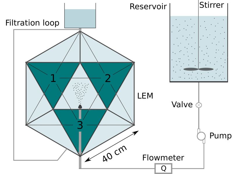
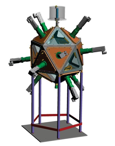
Lagrangian diffusion properties of a free shear turbulent jet 5
 (a) (b)

 Figure 1: (a) Three-dimensional CAD rendering of the Lagrangian Exploration Module.
 (b) Schematic of the hydraulic setup. Cameras 1, 2 and 3 are oriented orthogonal to the
 green faces labelled accordingly as 1, 2 and 3.

fundamental constants such as 0 , and the relevance of simple Lagrangian stochastic models
derived for homogeneous isotropic conditions (Sawford 1991).
 The aim of the present article is to address these unanswered questions through examination
of particle trajectories within a free jet. Three component trajectories of a turbulent water
jet (Re ' 230) are captured, with a measurement volume containing up to 45 diameters
downstream of the jet exit. Experimental methods provide sufficient temporal details to
analyse particle trajectories as well as adequate spatial resolution and interrogation volume
size to facilitate the application of basic Eulerian analysis. In section 2 the experimental setup
and methods are presented including the implementation of the Lagrangian particle tracking
and the stationarisation procedure that will be applied, inspired by Batchelor’s Lagrangian
self-similarity hypothesis. Section 3 is dedicated to basic Eulerian statistics, which are not
the main topic of this study but nevertheless allow the characterisation of key turbulence
properties (energy dissipation rate, Eulerian scales, Reynolds number, etc.) and their self-
similar behaviour. Section 4 includes results on the Lagrangian dynamics. In the context of
the previously discussed turbulent diffusion, emphasis is placed on second-order Lagrangian
statistics (velocity two-point correlation and structure functions), for which the Lagrangian
self-similarity compensation is tested and the estimate of the constant 0 is given. The
connections between Eulerian and Lagrangian scales are also considered in the framework
of classical stochastic modelling. Section 5 extends the discussion of Lagrangian statistics to
second-derivative dynamics where comparisons between key acceleration quantities and the
scaling constant, 0 , are presented. Finally, main conclusions are summarised in section 6.

2. Experimental methods
 2.1. Hydraulic setup
Experiments were performed in the Lagrangian exploration module (LEM) (Zimmermann
et al. 2010) at the École Normale Supérieure de Lyon. A vertically-oriented jet of water
is injected into the LEM, a convex regular icosahedral (twenty-faced polyhedron) tank full
of water, as seen in figure 1(a). The LEM is originally designed to generate homogeneous
isotropic turbulence when the twelve propellers on twelve of its faces are activated, however,
for this experiment, the LEM is only used as a tank as the optical access makes it an ideal
apparatus for three-dimensional particle tracking of a jet.

6 B. Viggiano and others
 (a) (b)
 LED panels

 α = 11◦
 β = 53◦

 jet θ = 72◦
 LEM
 • LED panels

 α
 Camera 1/2
 β
 θ jet

 LEM
 Camera 3

 Camera 1 Camera 2

 Camera 3

 Figure 2: Schematic of the optical setup: (a) top view and (b) profile view.

 A schematic of the hydraulic setup is included in figure 1(b). The vertical jet, injected with
a pump connected to a reservoir, is ejected from a round nozzle with a diameter = 4 mm. At
the nozzle exit, the flow rate is kept steady at ' 10−4 m3 /s, generating an exit velocity '
7 m/s, and in turn, a Reynolds number based on the diameter Re = / ' 2.8 × 104
with the water kinematic viscosity. Experiments are performed at ambient temperature.
By moving the vertical position of the nozzle, two locations are considered in order to
study near-field (NF) and far-field (FF) dynamics, with interrogation volumes spanning from
0 mm 6 6 120 mm (0 6 / 6 30) and 80 mm 6 6 200 mm (20 6 / 6 50),
respectively (the -axis is the jet axis with = 0 the nozzle exit position). For both regions,
the jet is sufficiently far from the walls of the tank to discount momentum effects from the
LEM onto the jet (Hussein et al. 1994), and thus a free jet is observed.
 The particles, seeding the jet during injection, are neutrally buoyant spherical polystyrene
tracers with a density = 1060 kg/m3 and a diameter = 250 µm. The reservoir is
seeded with a mass loading of 0.1% (reasonable seeding to observe a few hundred particles
per image) and an external stirrer maintains homogeneity of the particles. The quiescent
water inside the LEM is not seeded, therefore tracked particles are only those injected into
the measurement volume by the jet (although some tracers are always remaining in the tank).
The inlet valve is open some seconds before the recording, in such a way that the jet is
stationary but minimal particle recirculation occurs. The ratio of the particles diameter to
the Taylor microscale is always smaller than 1 and ranges from 0.3 (in the far-field) to 0.8
(in the near-field). The particles are not expected to deviate from tracer behaviour for velocity
statistics within the inertial range (Mordant et al. 2004a). The ratio to the Kolmogorov
length scale remains, however, larger than 1 and ranges from 9 (in the far-field) to 25 (in
the near-field). Finite size effects are therefore expected to influence small scale Lagrangian
dynamics and in particular acceleration statistics (Qureshi et al. 2007), as further investigated
in section 5.

 2.2. Optical setup
Three high speed cameras (Phantom V12, Vision Research) mounted with 100 mm macro
lenses (ZEISS Milvus) are used to track the particles. The optical configuration is shown in

Lagrangian diffusion properties of a free shear turbulent jet 7

 Figure 3: Measurement volume captured by the three camera setup for the near-field
 measurements (same measurement volume for the far-field measurements).

 800
 100

 90

 600
 80

 70

 400 60

 50

 40
 200
 30

 20

 0 200 400 600 800 1000 1200

 Figure 4: Detection of 705 particles on camera 2 in the near-field configuration (nozzle in
 the top left-hand corner). Inset: zoom on the boxed zone.

figure 2. The angles are related to the geometry of an icosahedron. The interrogation volume
is illuminated in a back light configuration with three 30 cm square LED panels oriented
opposite the three cameras. The spatial resolution of each camera is 1280 × 800 pixels,
creating a measurement volume of around 80 × 100 × 130 mm3 , as seen in figure 3, hence
one pixel corresponds to roughly 0.1 mm. The three cameras are synced via TTL triggering
at a frequency of 6 kHz for 8000 snapshots, resulting in a total record of nearly 1.3 s per run.
For each nozzle position (NF and FF), a total of 50 runs are performed to ensure statistical
convergence.

8 B. Viggiano and others

 Figure 5: Predictive tracking schematic. The solid line signifies the real trajectory. The
 dotted line (linear fit of the positions from frame − 4 to ) indicates the position
 extrapolation.

 2.3. Particle Tracking Velocimetry (PTV)
2.3.1. Particle detection
To create particle trajectories through PTV, two-dimensional images are first analysed to
measure the positions of the centres of the particles. The particle detection procedure used in
this study is an ad hoc process which uses classical methods of image analysis: non-uniform
illumination correction, morphological operations (opening), thresholding, binarisation and
centroid detection. An example of the camera image with detected particles is presented in
figure 4.

2.3.2. Stereoscopic reconstruction
After the particle centres for all images and all cameras have been determined, the actual three-
dimensional positions of the particles can be reconstructed, knowing that each camera image
is a two-dimensional projection of the measurement volume. More typically, methods based
on optical models are used to achieve real particle positions, but for this study a geometric
method developed by Machicoane et al. (2019) is used due to its increased precision and ease
of implementation. This method is based on an initial polynomial calibration, where each
position on a camera image corresponds to a line in real space (a line of possible positions in
three-dimensional space). The rays for each detected centre in the two-dimensional images are
computed based on the calibration then those rays are matched in space for all three camera
locations to create a volume of particles in real space. The matching algorithm employed
was recently developed by Bourgoin & Huisman (2020). To create the largest convex hull
possible which is dictated by the orientation of the cameras, matching of particle position
based on the intercept of only two rays (i.e. two cameras of the three total) is accepted.
The possibility of overlapping of particles in one dimension, two matches per ray, is also
admitted in this algorithm. However this allows the inclusion of non-existent ghost particles.
Fortunately, these ghost particles do not form persistent trajectories and therefore they are
removed when the trajectories are formed in the next step. The tolerance to allow a match is
50 µm (calibration accuracy around 1 µm).

2.3.3. Tracking
The stereoscopic reconstruction gives a cloud of points for every time step. The goal of the
tracking is to transform this cloud into trajectories by following particles through time. To
track the position of a considered particle as it moves among numerous other particles, the
simplest algorithm is to consider the nearest neighbour: if one considers a particle in frame
 , its position in frame + 1 is the nearest particle in frame + 1. But, for increased mass
loading of particles, the trajectories are tangled, as observed in this study. Moreover, several
points are “ghost” particles and should not be tracked. Thus advanced predictive tracking
methods are generally employed (Ouellette et al. 2006a). The trajectories are assumed to

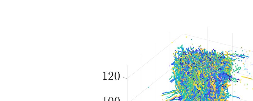
Lagrangian diffusion properties of a free shear turbulent jet 9

 Figure 6: Near-field jet: 95 055 trajectories longer than or equal to 10 frames (one colour
 per trajectory, one movie considered).

be relatively smooth and self-consistent, i.e. there are no severe variations in velocity and
therefore past positions give accurate indications of future positions (Guezennec et al. 1994).
If one considers a particle at frame , its position in frame + 1 can be extrapolated and
finally the nearest neighbour approach is employed based on the extrapolated position. In the
present study, the extrapolated position is determined by fitting the previous five positions
from frame − 4 to with a simple linear relation (i.e. velocity), as indicated in figure 5. If
there are less than five positions, the available positions are used. A maximum distance of
1 mm between extrapolated position and real position is applied to continue the trajectories in
order to avoid the tracking of absurd trajectories. If the same particle is the nearest neighbour
for two different tracks, the nearest trajectory is chosen and the other trajectory is stopped.

 2.4. Post-processing of the trajectories
The tracking of particles results in a set of trajectories for each of the 50 experimental runs. A
minimum trajectory length of 10 frames is required to remove presumably false trajectories.
Some real trajectories are also removed, but their statistical value is negligible. Finally, the
coordinate basis is adapted by aligning the -axis with the jet axis and centring it in and 
directions. Positions and velocities are computed in adapted cylindrical coordinates ( , , )
with the axial coordinate, the radial one and the circumferential one. A visualisation of
tracks is shown in figure 6. It can be noted that most trajectories come from the nozzle (where
they are injected) and very few come from the outside and are entrained in the jet (visible in
figure 6 as radial trajectories towards the jet). The full data set for the near-field comprises
4.2 × 106 trajectories longer than or equal to 10 frames, which corresponds to 1.0 × 108
particle positions. For the far-field, it comprises 6.1 × 106 trajectories and 1.6 × 108 particle
positions.
 The trajectories reconstructed by the tracking algorithm always exhibit some level of noise
due to errors eventually cumulated from particle detection, stereo-matching and tracking.
It is important to properly handle noise, in particular when it comes to evaluating statistics
associated to differentiated quantities (particle velocity and acceleration). Two techniques

10 B. Viggiano and others
 (a) (b)
 30

 25

 20

 15

 5m/s

 10
 0 2 4 6

 Figure 7: (a) Vector field of the field for the normalised locations, including the
 half-width of the jet (−−), 1/2 , at all downstream locations for the near-field. (b) Contour
 representations of the local standard deviations (left) and (right) for the axial and
 radial velocity components for near-field locations.

are implemented to do so. For all Eulerian statistical analysis requiring the estimate of
local velocity, the trajectories are convolved with a first-order derivative Gaussian kernel
with a length of 6 time instances and a width of 2 (ad hoc smoothing parameters)
(Mordant et al. 2004b). For all two-time Lagrangian statistical analysis (correlation and
structure functions), an alternative noise reduction method, presented by Machicoane et al.
(2017a,b), is implemented to obtain unbiased statistics based on an estimation from discrete
temporal increments of position, without requiring explicit calculation of individual trajectory
derivatives. For example, to compute the noiseless Lagrangian two-point correlation of
velocity, ˆ ˆ , the first-order increments are considered as follows:
 ( , ) = ˆ ˆ ( ) 2 + h( ) 2 i + O ( 3 ), (2.1)
where is the temporal increment of the signal over a time with = ( + ) − ( ) =
 ˆ + . The circumflex signifies the real (noiseless) signal and the noise is denoted as 
(assumed to be a white noise). From the presented relationship, the noiseless correlation
function of velocity ˆ ˆ ( ) can be extracted from the correlation of measured position
increments , exploring its polynomial dependency with at the lowest (quadratic) order
and neglecting higher-order terms (i.e. O ( 3 )), by applying a simple polynomial fit of
 1 2 + 2 . This method, called “ -method” in the following, allows the estimation, with
increased accuracy and less sensitivity to noise, of statistics of differentiated quantities
(and hence to explore small scale mechanisms), without actually requiring estimation of
derivatives, but by simply considering position increments at various temporal lags. More
information is provided in Machicoane et al. (2017a,b).

 2.5. Stationarisation techniques
To address the Lagrangian instationarity (related to the Eulerian inhomogeneity) of the flow,
methods are taken according to the proposed self-similarity of a turbulent jet by Batchelor
(1957), i.e. based on the transformation of the Lagrangian velocity and time scales of a
particle at a given time after it has been released from a point source. Equation (1.2)
provides a relationship to achieve proper stationarisation. For this study, the fluctuating
stationarised velocity is obtained by subtracting the local Eulerian velocity (and assuming

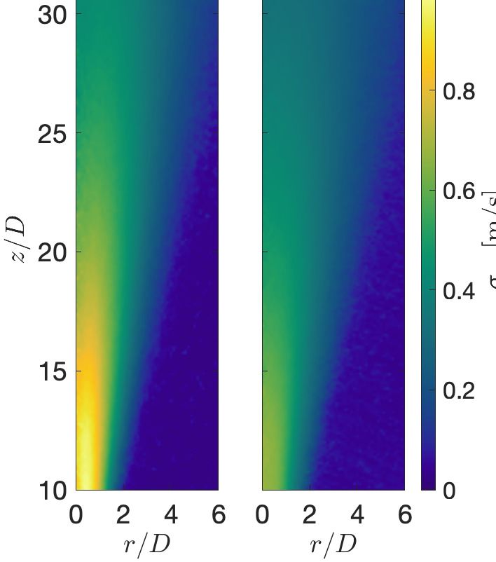
Lagrangian diffusion properties of a free shear turbulent jet 11
cylindrical symmetry of the jet, hence neglecting the dependence on spatially averaged
quantities), ( , ), and scaled by the local standard deviation, ( , ). Explicitly,
 ( ) − ( ( )) ( ) − ( , )
 ˜ ( ) = = . (2.2)
 ( ( )) ( , )
The local standard deviation is an optimal choice for compensation as it generalises the
methods presented in Batchelor (1957), where a specific decay rate (Batchelor assumed a
power-law) is required for stationarisation. This velocity ˜ takes the mean drift and decay into
account although the term becomes dimensionless as a result. For this reason, for all statistical
calculations of dimensional quantities (such as the turbulent dissipation rate) inferred from
this analysis, velocity is redimensionalised through multiplication with the average local
standard deviation within the considered measurement region or location. For transparency,
the Eulerian mean and standard deviation velocity fields used for the stationarisation are
presented in figure 7 (figure 7(a) the mean velocity as a vector field and figure 7(b) the
standard deviation of the axial and radial velocity components). The half-width of the jet,
 1/2 ( ), where ( , = 1/2 ( )) = 21 ( , = 0), is included in the Eulerian mean velocity
field as the dashed line to provide clarity to the sampling methods based on this quantity,
as discussed in sections 3 and 4. Note that Lagrangian velocity components are used for
the Eulerian statistical characterisation therefore the stationarisation technique described is
required for all analyses presented in the study. For clarity, herein the tilde is omitted and the
compensated Lagrangian velocity is denoted as ( ) for the remainder of the article.

3. Eulerian velocity statistical analysis
This section aims to extract flow parameters such as length scales and energy dissipation rate
from different Eulerian statistics: second-order structure functions and two-point correlation
functions. The jet flow is inhomogeneous, therefore these quantities depend on and . Focus
is placed on centerline statistics for the Eulerian characterisation of the jet, limited to radial
distances up to 1/2 and consideration of only the -axis evolution is used to characterise the
main property of the base turbulence.

 3.1. Eulerian second-order structure functions
Structure functions are commonly used to describe multi-scale properties of turbulence
through a statistical representation of a flow quantity with a given spatial or temporal
separation. In the Eulerian perspective, longitudinal velocity structure functions of order
 are defined as
 
 − k ( , ) = h[ k ( , )] i = h[ k ( + ) − k ( )] i, (3.1)
where k is computed over two points, one at , the other at + , with k defined as
the single longitudinal component of Eulerian velocity along . The h·i denotes ensemble
averaging.
 In homogeneous isotropic stationary turbulence (HIST), Kolmogorov phenomenology K41
(Kolmogorov 1941) predicts for the second-order structure function in the inertial range,
scales between the Kolmogorov scale, , and the integral length scale, , that:

 2 ( Δ) 2/3
 2− k (Δ) = h[ k ( , Δ)] i = 2 , (3.2)
 2k
with the average energy dissipation rate per unit mass and 2 ' 2.0 (Pope 2000). The
 2k denominator (the variance of longitudinal velocity component) has been added here

12 B. Viggiano and others
in the right hand term to account for the fact that the stationarised velocity according to
 (Δ)
transformations (2.2) is considered. Alternatively, the transverse structure function 2−⊥
can be considered where increments are taken for the velocity components perpendicular
 (Δ) follows the same K41
to the separation vector. In HIST, within the inertial range, 2−⊥
 4
scaling but with a constant 2⊥ = 3 2 . Previous studies have found that these relations a
priori established for HIST, apply reasonably well to the inertial scales of turbulent jets, in
spite of the large scale inhomogeneity and anisotropy (see for instance Romano & Antonia
(2001)). In the sequel relation (3.2) is used together with the relation 2⊥ = 43 2 to analyse
longitudinal and transverse structure functions in the jet.
 Within the jet (cylindrical coordinates), the longitudinal second-order structure function
is usually estimated, near the centerline, based on the axial component of the velocity:
 2
 2− , k ( , ) = h[ ( + , ) − ( , )] i, (3.3)
with the fluctuating axial velocity (recall that the stationarisation described in section 2.5
is applied) and the axial distance between the two considered points (the explicit 
dependency is kept here to emphasise the streamwise inhomogeneity of the jet centerline
statistics). This is, for instance, the quantity typically measured when using hot-wire
anemometry (sensitive to the streamwise velocity component) combined with the Taylor
frozen field hypothesis.
 To explore the streamwise evolution of Eulerian properties of the jet, a set of data (particle
velocities) is considered for a given position, which falls within a short cylinder (disk), D ,
of limited height (0.5 mm in the -direction) and a radius of 1/2 ( ) for statistical analysis. The
disk radius is chosen to include sufficient particles for statistical convergence but, in being
limited to the half-width, the volume does not encompass particles from the turbulent/non-
turbulent interface. This gives a canonical description of turbulent properties representative
of the centerline of the jet. Consideration of statistics in a thin disk allows the more detailed
exploration of dependence of statistical quantities, however this sampling technique forbids
exploration of values over a range relevant to estimate 2− , 
 k
 ( , ) at inertial scales. To
overcome this issue, two strategies are considered: (i) Still based on the axial -component
 
of the velocity, 2− ,⊥ ( , ), the transverse structure function of (with the separation
vector taken within the plane of the disk) is estimated in lieu of 2− , 
 k
 ( , ); (ii) For
radial velocities, the longitudinal structure function is considered through use of the velocity
components perpendicular to the -axis (i.e. within the sampling disk D ), projected onto
the increment vector within the disk D . This is denoted as 2− 
 , k
 ( , ) (where the
subscript recalls that only velocity components perpendicular to are considered). For
any redimensionalization of a Eulerian quantity, the averaged standard deviation within a
respective disk, h i D , is employed. For brevity this is herein denoted as for all Eulerian
calculations.
 The discussions of this subsection (and in the two following) illustrate the extraction of the
main Eulerian turbulent properties (and of their streamwise evolution) based on 2− ,⊥ ( , ).
The same analysis was also repeated based on 2− , k ( , ), the details of which are not
 
provided for brevity. Analysis follows the same recipe as is described for 2− ,⊥ ( ), and
the main extracted turbulent parameters from these two estimates will be discussed and
compared in section 3.3.
 The transverse structure function based on at a given position is estimated as
 
 2− ,⊥ ( , ) = h[ ( + ) − ( )] 2 i D , (3.4)
where the average is taken over pair of particles within the disk D separated by a

Lagrangian diffusion properties of a free shear turbulent jet 13
 (a) (b)

 Figure 8: Eulerian second-order structure functions of the axial velocity on the axis,
 
 (a) uncompensated 2− ,⊥ ( , ) 2 and (b) compensated
 
 ( 2− ,⊥ ( , ) 2 / 43 2 ) 3/2 / (the solid lines are the plateaus to extract ), for the four
 denoted downstream locations.

vector . Note that, given the reduced height of the disk (not exceeding two particle
diameters), is within an acceptable approximation perpendicular to the axis, ensuring
that equation (3.4) indeed corresponds to a transverse structure function (except maybe for
the smallest separations, comparable to the disk height).
 
 2− ,⊥ ( , ) is computed for different positions (in the near and far-fields of the
jet) and shown in figure 8(a). As explained in section 2.5, while the stationarised (hence
 
dimensionless) velocity is used for all estimates, 2− ,⊥ is made dimensional by multiplying
it by the square of , the standard deviation of within D (see table 1). This redimen-
sionalisation is required in order to extract the dimensional value of , and the associated
derived parameters (in particular the dissipation scales and Taylor micro-scale). To this
end, figure 8(b) includes the compensated structure function ( 2− ,⊥ ( , ) 2 / 43 2 ) 3/2 / 
(measurements by Romano & Antonia (2001) suggest that at in spite of the large scale
anisotropy, the isotropic relation 2⊥ = 43 2 applies reasonably well for the inertial scale
dynamics of the jet). Well defined plateaus, corresponding to inertial range dynamics, are
observed from which the dissipation rate can be extracted according to equation (3.2). The
subscript in simply refers to the fact that this estimate is based on the axial component
of the velocity. It will be compared later with , the estimate from 2− . It can be seen
 , k
that, as the location downstream increases, the plateau of the second-order structure function
(and hence ) decreases, due to the streamwise decay of turbulence along the jet.
 It is noted that small scales (typically for < 10−3 m) are not statistically well converged.
This is due to the lack of statistics for pairs of particles with very small separation due to the
moderate seeding of particles used for the Lagrangian tracking.

 3.2. Eulerian two-point correlation functions
The second-order Eulerian statistics shown in the previous section from the structure
functions can be equivalently investigated in terms of the two-point correlation function.
The correlation of axial velocity can indeed be obtained via the non-dimensional second-
 
order structure function, − ,⊥ ( , ) = 1 − 2− ,⊥
 ( , )/2, to depict the evolution of
the velocity interactions through space. The results from the near-field and far-field are
presented in figure 9. The curves are ordered depending on their downstream location .

14 B. Viggiano and others
 1

 0.8

 0.6

 0.4

 0.2

 0

 0 0.002 0.004 0.006 0.008 0.01

 Figure 9: Normalised two-point spatial correlation of the Eulerian axial velocity on the
 
 axis, − ,⊥ 
 ( , ) = 1 − 2− ,⊥ ( , )/2.

 100

 80

 60

 40

 20

 0
 15 20 25 30 35 40 45

 Figure 10: Evolution of along the jet axis.

The location nearest the jet exit, / = 15, exhibits a rapid decorrelation. As the flow
advances downstream, the turbulent length scales grow, resulting in a dynamics which
remains correlated over longer distances, as seen by the / = 45 profile. This trend can
be investigated quantitatively
 ∫∞ using the Eulerian correlation length (or Eulerian integral
scale) ,⊥ ( ) = 0 − ,⊥
 ( , ) d . Recall that transverse and longitudinal correlation
lengths are kinematically related in HIST by ,k = 2 ,⊥ (Pope 2000). Since most
studies in the
 ∫ ∞literature refer to the longitudinal length, the present study will then consider
 ( ) = 2 0 − ,⊥
 ( , ) d , avoiding the ⊥ or k subscripts. However, it is noted that
measurements by Burattini et al. (2005) suggest that the ratio may actually be slightly lower
than 2, and closer to 1.8 in free shearing jets due to large scale anisotropy.

 3.3. Evolution of Eulerian parameters
The evolution of , estimated from the plateaus of the compensated second-order structure
functions (figure 8(b)), is represented in figure 10. There exists a tendency of 1/ 4 (more
clearly visible in figure 11(c)), as expected for canonical self-similar jets. The observed
consistency in the values and shape of the profiles between the near and far-field experimental
locations, validates the presented values from the independent measurements carried over
the overlapping region.
 From the dissipation rate , other relevant parameters of the flow field can be extracted,
namely the Kolmogorov time scale, = ( / ) 1/2 , and length scale, = ( 3 / ) 1/4 , as

Lagrangian diffusion properties of a free shear turbulent jet 15

 / Re 
 [m/s] [W/kg] [µm] [ms] [µm] [mm] [ms] [m/s] [W/kg] [mm] [ms]
 15 0.80 104.7 9.9 0.098 304 245 2.2 2.8 0.57 63.9 1.7 2.9
 25 0.51 16.1 15.8 0.249 491 250 4.4 8.6 0.38 14.6 2.0 5.3
 35 0.35 4.5 21.7 0.472 643 226 5.6 16.0 0.28 5.7 3.6 13.0
 45 0.28 1.7 27.8 0.774 825 227 7.8 28.2 0.22 2.4 5.1 23.2

 Table 1: Eulerian parameters of the jet on the axis for different / positions.

 (a) (b) (c)
 0.8 2
 10 7
 -1 1
 0.6
 -4 6
 5
 10 1 4
 0.4
 3
 0
 10
 20 30 40 20 30 40 20 30 40

 Figure 11: (a) The standard deviation averaged within the disk D , (b) the dissipation rate
 and (c) the integral length scale for the axial component of velocity for all downstream
 locations. Power-law relation is given as dashed line.

well as the Taylor microscale, = (15 2 / ) 1/2 , and the Taylor-based Reynolds number
Re = / , both of which assume HIST. Further, large length and time scales are
obtain from the two-point correlation
 ∫∞ profiles in figure 9. For a more accurate estimate of the
correlation length, ( ) = 2 0 − ,⊥
 ( , )d , the integral of the correlation functions
is based on a fit of the curves shown in figure 9 using a Batchelor type parametrisation
(Lohse & Müller-Groeling 1995). Recall that the factor 2 is the HIST correction that relates
the transverse correlation (given by the integral of − ,⊥ ) to the longitudinal one. The
calculated shall therefore be interpreted as the longitudinal integral scale associated to
the component of velocity. The integral time scale is then computed as = / . All
relevant quantities of the jet have been accumulated for the considered streamwise locations
in table 1. The streamwise evolution for the velocity standard deviation, dissipation rate and
integral scale are also shown in figure 11, where the well known self-similar power-law
profiles can be seen.
 This brief characterisation of basic Eulerian properties is concluded by reporting the
similarly employed analysis performed on 2− 
 , k
 ( , ) (where rather than , components
of velocity perpendicular to the z-direction are considered). This leads to estimates of the
dissipation rate (and derived quantities) and of the integral length scale and time scale,
 and . Results are included in table 1. The dissipation rate for the radial velocity is
lower than the axial component near the exit of the jet, but declines more slowly as the jet
develops, resulting in similar values for and at / > 25. As a result, in this region
dissipation scales are found almost identical with both estimates. This supports the idea that
small and inertial scales are nearly isotropic. The large scales show however a certain degree
of anisotropy, in particular regarding the integral length scale and in a lesser degree the
integral time scale which are found larger for the -component than for the -components.

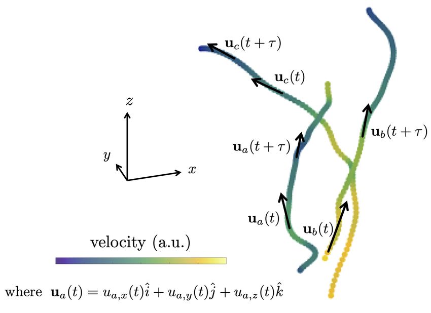
16 B. Viggiano and others

 Figure 12: Schematic of the Lagrangian velocity increment in a Cartesian coordinate
 system for a given time lag .

4. Lagrangian velocity statistical analysis
In this section the Lagrangian statistics of the jet dynamics are investigated with a particular
focus on second-order statistics (namely velocity second-order structure function and two-
point correlation function), which are key ingredients to model turbulent diffusion, as
discussed in the introduction. In particular, the relevance of Batchelor’s Lagrangian self-
similar stationarisation idea is further assessed.

 4.1. Lagrangian second-order structure functions
The application of the known Kolmogorov K41 phenomenology for HIST, generally applied
to Eulerian inertial scaling, can be extended to the Lagrangian framework (Toschi &
Bodenschatz 2009), where dynamics is investigated as a function of temporal increments
along particle trajectories (see figure 12). Namely, for the second order Lagrangian structure
function, this reads (for the stationarised velocity defined by relation (2.2)):
 
 2, ( ) = h[ ( + ) − ( )] 2 i = 0 2 , (4.1)
 
within the the inertial range (   ), where is a velocity component ( = , or ,
by symmetry, statistics along and are identical and equivalent to statistics of the radial
 -component of velocity), and is the Lagrangian integral time scale, which is expected
to be related to the Eulerian integral time (this point will be further deepen later). Note
that while for the Eulerian structure functions, spatial velocity increments were computed
between pairs of particles and then averaged, now, for Lagrangian analysis, temporal velocity
increments are computed on each individual trajectories before being averaged. In this study,
the nature of this scaling is revisited as well as the value of the constant 0 when the
stationarised velocity presented in section 2.5 is considered. In order to address the role
of jet anisotropy (in particular regarding the value of 0 and 0 ), the statistics for the
axial and radial components of velocity are considered separately. Recall also that in lieu
of Gaussian filtering previously applied to the Eulerian structure functions, the -method
presented in section 2.4 is implemented, which has been shown to better handle noise issues
for Lagrangian velocity statistics estimates (Machicoane et al. 2017a).
 Figure 13(a) presents the corresponding curves for 2, ( ) at the four different downstream

locations. For each location , the ensemble selected for the Lagrangian statistics consists
of all trajectories passing through a small sphere, S centred at downstream position 
along the jet centerline, with a radius of 1/2 ( )/3. This volume allows sufficient particles for

Lagrangian diffusion properties of a free shear turbulent jet 17
 (a) (b)
 100

 10
 0 100
 10-2

 -5
 10
 10 -4 10 -3 10 -2
 -4 -1
 10 10
 -2 0 -3 -2
 10 10 10 10

 Figure 13: Lagrangian second-order structure functions of the axial velocity on the axis,
 estimated at four downstream locations ( / = 15, 25, 35, and 45). (a) Non-dimensional
 ( ) as a function of the non-dimensional time / 2
 2, (dimensional 2, ( ) as a
 ( ) 2 /( ), for the denoted
 function of time in inset) and (b) compensated 2, 
 downstream locations. The universal scaling constant, 0 , can be extracted from the
 plateau of the compensated structure functions.

convergence of statistics yet does not overlap in the axial direction as the half-width increases.
Similar to methods presented in the Eulerian framework, the averaged standard deviation
from within each respective sphere, h i S , is used for redimensionalization of Lagrangian
quantities when necessary (for calculation of 0 ) and denoted simply as . All curves
exhibit a transition from a dissipative behaviour at small time lags (where 2, ∝ 2 ) to the

inertial range (where 2, ∝ ). The main figure shows the structure function in stationarised

variables, while the inset provides the same data but non-stationarised. Several interesting
points emerge:
 • Effect of stationarisation at inertial scales. The non-stationarised statistics (inset
of figure 13(a) are widely spread while the stationarised statistics (main figure) collapse
reasonably well, in particular in the far-field ( / > 25). Similarity between the curves is
improved for the inertial range dynamics (which presents similar trends even at distances
 / & 20), but less adequate for the small scale dissipative dynamics, for which the
collapse becomes reasonable only at far downstream locations ( / > 35). This suggests that
the stationarisation procedure is efficient to retrieve self-similar inertial range Lagrangian
statistics in the far-field (in Batchelor’s sense, meaning that Lagrangian statistics become
independent of the downstream position as particles travel along the jet), while discrepancies
remain in the small scales until the very far-field.
 • Small scale dynamics discrepancies. In the Lagrangian framework, the small scale
dynamics of structure functions is associated to particle acceleration statistics. Figure 13(a)
therefore suggests that stationarised acceleration statistics eventually fall in line, but only in
the very far-field (curves at / = 40 and 45 almost perfectly collapse). As will be observed
in section 5, acceleration statistics are strongly affected by the finite size of the particles,
which in our study remains much larger than the dissipation scale of the flow ( / = 25 at
 / = 15 and 9 at / = 45). Although further investigation focusing specifically on the
small scale dynamics would be required (which is not the scope of the present article, mostly
motivated by applications to diffusion which is primarily driven by inertial and large scale
behaviour), it is probable that the observed discrepancy at small scales reflects these finite
size effects. This is supported by the fact that as considered positions are farther downstream
(where / gets smaller and hence finite particle size effects disappear), the stationarised

18 B. Viggiano and others
 (a) (b)
 1
 0.8

 0.6
 0.8
 0.4

 0.2
 0 2 4 6 8
 0.6 10 -3

 0.4

 0.2
 0 0.5 1 1.5 2 2.5 3

 Figure 14: Normalised Lagrangian correlation of the axial velocity for the compensated
 time lag / . Inset provides the Lagrangian correlation as a function of the dimensional
 time lag for the same seven downstream locations previously considered. Locations are
 (a) along the centerline ( = 0) and (b) at the jet half-width ( = 1/2 ) for all downstream
 positions.

acceleration dynamics seems to better converge to a single curve. Accelerations statistics and
finite size effects will be further discussed in section 5.
 • Large scales dynamics. By construction, the second order structure function of the
stationarised velocity should reach, in the large scales, an asymptotic constant value of
2 as the Lagrangian dynamics becomes fully decorrelated. This asymptotic regime is not
reached in our data, where 2 reaches at best values of order 1, without exhibiting an
asymptotic decorrelated plateau. This is due to the lack of statistics for long trajectories.
One of the well-known difficulties of Lagrangian diagnosis is indeed the capacity to obtain
sufficiently long trajectories allowing to explore the large scale dynamics. In the present
study, most trajectories are efficiently tracked over a few tens of frames at most (very few are
over hundreds of frames). At the operating repetition rate of 6000 frames per second, this
corresponds to trajectories at most 10 ms long, what represents (according to table 1) a few
Eulerian integral times scales in the near-field, and only a fraction of this integral scale in the
far-field, where only a part of the inertial range dynamics is accessible. In subsection 4.2, it
is demonstrated that large scale behaviour (and the effect of stationarisation on it), can still
be addressed by estimating the Lagrangian correlation time scales.
 • Estimate of 0 constant. Figure 13(b) shows the compensated structure functions,
 ( ) 2 /( ), built with values found in the Eulerian analysis (for consistency
 2, 
regarding possible anisotropy effects, the estimate of dissipation rate based on Eulerian
statistics of corresponding components is used). Based on relation (4.1), within the inertial
range the value of 0 can be extracted from the plateau of the curves. The value of the
plateau is observed to saturate, as considered positions reach farther towards the far-field,
at a value of 0 ' 3.2. The downstream evolution of 0 will be further discussed in the
coming sections.
 , based on the radial component of velocity.
 All observations also apply to estimates of 2, 
Quantitative comparison of the downstream evolution of 0 and 0 will be detailed in
section 4.3.

 4.2. Lagrangian two-point correlation functions
The two-point correlation functions of the Lagrangian axial velocity as a function of the
compensated time lag, / , are presented in figure 14(a) where − ( ) = h ( +
 ) ( )i. It can be seen that, as for the structure functions previously discussed, the
stationarisation results in a remarkable collapse of the correlation functions, in particular
at / > 20. Note that the small scale discrepancy observed for 2, is also expected

Lagrangian diffusion properties of a free shear turbulent jet 19

 / 0 [ms] / 0 [ms] / 
 15 1.4 4.5 0.6 1.9 1.4 2.1
 25 2.7 5.3 1.6 3.2 2.3 2.3
 35 3.2 11.1 1.5 3.0 5.3 2.5
 45 3.0 15.9 1.8 2.8 8.9 2.6

 Table 2: Lagrangian parameters of the jet on the axis for different / positions.

to be present for the correlation function, which carries essentially the same information;
it is however less emphasised due to the linear (rather than logarithmic) scale used to
represent the correlation function. The observed agreement between the two-point correlation
functions confirms again the Lagrangian self-similarity hypothesis at inertial scales, resulting
in two-point correlation functions of the stationarised variables which do not depend on the
downstream position of the particles as they evolve along the jet (beyond / & 20).
 Although the shortness of the trajectories does not allow to directly explore the large scale,
fully decorrelated, regime (where , vanishes), the observed collapse at intermediate
scales allows speculation that the self-similarity hypothesis may also extend to the large
scales. This would lead, in particular,
 ∫∞ to a univocal relation between the Lagrangian
correlation time (defined as = 0 , ( ) d ) and the Eulerian timescale at all positions
 
along the jet (except in the very near-field, where Lagrangian two-point correlation clearly
deviates). This point will be further tested in the subsection 4.3 where we estimate based
on appropriate fits (exponential or double exponential (Sawford 1991)) of the Lagrangian
two-point correlation, supporting the validity of self-similarity in the large scales and the
univocal link between and .
 The subsection is concluded by providing, in figure 14(b), a test of the Lagrangian self-
similarity hypothesis when off-axis dynamics is considered. The original stationarisation
proposed by Batchelor (1957) used centerline power-laws for a self-similar jet to compensate
the Lagrangian velocity and time. As discussed in section 2.5, these formulas have been
generalised (compatible with Batchelor’s approach in the centerline), using actual local
measurements of Eulerian properties rather than prescribed centerline power-laws. The
stationarisation transformations can therefore be applied at any arbitrary position along
particles trajectories. Figure 14(b) explores the application of the proposed stationarisation
considering trajectories passing through a ball centred off-axis, at a radial location of
 = 1/2 ( ), instead of = 0. As for the centerline analysis, the correlation functions of the
stationarised variables collapse for all locations / > 20. This substantiates the generalised
stationarisation technique, and its application to locations beyond the centerline. Although
the present study focus on diffusion of particles near the jet centerline, this result motivates
future dedicated studies to explore more deeply the generalised Lagrangian stationarisation
for off-axis statistics as well as for other inhomogeneous flows (such as von Kármán flows,
which are widely used for Lagrangian studies of turbulence).

 4.3. Evolution of Lagrangian parameters
This subsection provides the estimates of 0 and , their streamwise evolution along the jet
centerline, their connection to Eulerian properties of the jet and the reliability of Lagrangian
stochastic models derived for HIST (Sawford 1991) to address the stationarised Lagrangian
dynamics of the jet. Investigations are made into these quantities for both axial and radial
components of the velocity.
 Table 2 presents these Lagrangian parameters of the jet for different locations in the