Parametric numerical study of passive scalar mixing in shock turbulence interaction
←
→
Page content transcription
If your browser does not render page correctly, please read the page content below
Downloaded from https://www.cambridge.org/core. IP address: 46.4.80.155, on 06 Nov 2020 at 08:03:04, subject to the Cambridge Core terms of use, available at https://www.cambridge.org/core/terms. https://doi.org/10.1017/jfm.2020.292
J. Fluid Mech. (2020), vol. 895, A21. c The Author(s), 2020. 895 A21-1
Published by Cambridge University Press.
This is an Open Access article, distributed under the terms of the Creative Commons Attribution
licence (http://creativecommons.org/licenses/by/4.0/), which permits unrestricted re-use, distribution, and
reproduction in any medium, provided the original work is properly cited.
doi:10.1017/jfm.2020.292
Parametric numerical study of passive scalar
mixing in shock turbulence interaction
Xiangyu Gao1, †, Ivan Bermejo-Moreno1, † and Johan Larsson2
1 Aerospace and Mechanical Engineering Department, University of Southern California, Los Angeles,
CA 90089, USA
2 Mechanical Engineering Department, University of Maryland, College Park, MD 20742, USA
(Received 11 September 2019; revised 28 January 2020; accepted 7 April 2020)
Turbulent mixing of passive scalars is studied in the canonical shock–turbulence
interaction configuration via shock-capturing direct numerical simulations, varying
the shock Mach number (M = 1.28–5), turbulence Mach number (Mt = 0.1–0.4),
Taylor microscale Reynolds number (Reλ ≈ 40, 70) and Schmidt number (Sc = 0.5,
1, 2). The shock-normal evolution of scalar variance and dissipation transport
equations, spectra and probability density functions (PDFs) are examined. Scalar
dissipation, its production and destruction increase across the shock with higher
M, lower Mt and lower Reλ . Mixing enhancement for different flow topologies
across the shock is studied from changes in the PDFs of velocity gradient tensor
invariants and conditional distributions of scalar dissipation. The proportion of the
stable-focus-stretching flow topology is the highest among all the topologies in
the flow both before and after the shock. Unstable-node/saddle/saddle topology
is the most dissipative throughout the flow domain, despite variations across the
shock. Preshock and postshock distributions of the alignment between the strain-rate
tensor eigenvectors and the scalar gradient, vorticity and the mean streamwise vector
conditioned on flow topology are studied. A novel barycentric map representation is
introduced for a more direct visualization of the alignments and conditioned scalar
dissipation distributions. Interaction with the shock increases alignment of the scalar
gradient with the most extensive eigenvector, decreasing it with the most compressive,
which is still dominant. The barycentric map of the passive scalar gradient also
reveals that, across the shock, the most probable alignment between scalar gradient
and strain eigendirections converges towards the alignment that provides the most
dissipation. This also leads to an enhancement of scalar dissipation immediately
downstream of the shock.
Key words: turbulent mixing, compressible turbulence, shock waves
1. Introduction
The enhanced mixing that results from the amplification of turbulence across a
shock wave can be critical in applications such as hypersonic propulsion (supersonic
† Email addresses for correspondence: xiangyug@usc.edu, bermejom@usc.edu
Downloaded from https://www.cambridge.org/core. IP address: 46.4.80.155, on 06 Nov 2020 at 08:03:04, subject to the Cambridge Core terms of use, available at https://www.cambridge.org/core/terms. https://doi.org/10.1017/jfm.2020.292
895 A21-2 X. Gao, I. Bermejo-Moreno and J. Larsson
combustion ramjets) and inertial confinement fusion. The canonical shock–turbulence
interaction (STI) configuration has been extensively studied theoretically, experimentally
and through numerical simulations. However, few studies have concentrated on
quantifying the effects of the interaction on scalar mixing, in particular as the
relevant physical parameters and regime of the interaction are changed, which is the
focus of the present work.
Theoretical approaches to study STI include linear interaction analysis (LIA) (Moore
1953; Ribner 1953, 1954; Livescu & Ryu 2016; Jackson, Kapila & Hussaini 1990;
Jackson, Hussaini & Ribner 1993; Wouchuk, Huete & Velikovich 2009; Quadros,
Sinha & Larsson 2016a,b) and rapid distortion theory (RDT) (Lele 1992; Cambon,
Coleman & Mansour 1993; Jacquin, Cambon & Blin 1993; Kitamura et al. 2016).
More recently, dimensional and similarity analyses were put forward based on a
quasi-equilibrium assumption of instantaneous local adjustment of the shock, seen as
a collection of infinitesimal laminar shocks (see Donzis 2012a,b; Chen 2018). In the
last two decades, a number of developments have made LIA suitable for the analysis
of more complex physics, including mixing, chemical reactions and real gas effects
(Griffond 2005, 2006; Huete, Sánchez & Williams 2013, 2014; Hejranfar & Rahmani
2019).
Shock-driven mixing enhancement has been observed in experiments (Andreopoulos,
Agui & Briassulis 2000). In the study of the effects of shock propagation on the
properties of a random medium, Hesselink & Sturtevant (1988) observed enhanced
mixing in the shock-processed, strongly compressed fluid. Marble, Hendricks &
Zukoski (1989) found faster mixing by baroclinic vorticity in the interaction of
weak oblique shocks and cylindrical jets of hydrogen in air. Menon (1989) observed
an accelerated spreading of shear layers downstream of interactions with shock
waves, indicative of better mixing. Experiments have also confirmed theoretical LIA
predictions on the amplification of small-scale turbulence across the shock (Barre,
Alem & Bonnet 1996; Agui, Briassulis & Andreopoulos 2005; Andreopoulos 2008),
concluding that the flows downstream of shocks become more vortex dominated than
their upstream counterparts (Andreopoulos 2008).
Numerical simulation, mostly direct numerical simulation (DNS), has become
commonplace in the study of STI, complementing experiments and theory. Linear
interaction analysis predictions of turbulence kinetic energy (TKE) and transverse
vorticity variance amplification, and decreased turbulence length scales across the
shock have been confirmed in direct numerical simulations (Lee, Lele & Moin 1993,
1994; Ryu & Livescu 2014). Likewise, simulations have confirmed the saturation of
TKE amplification for Mach numbers larger than 3 (Lee, Lele & Moin 1997), which
could impose limits on achievable shock-induced mixing enhancements for increasing
shock strength. But simulations have also elucidated nonlinear effects that cannot
be predicted by LIA, such as the rapid postshock TKE evolution and the role of
upstream acoustic/vorticity/entropy fluctuations and temperature–velocity correlations
on postshock TKE amplification and turbulence length scales (Hannappel & Friedrich
1995; Mahesh, Lele & Moin 1997; Jamme et al. 2002). Different STI regimes have
been identified through parametric DNS studies to depend on the relative strength
of the incoming turbulence and the shock, characterized by the ratio Mt /(M − 1)
(Larsson & Lele 2009; Donzis 2012b; Larsson, Bermejo-Moreno & Lele 2013)
or Re−1/2
λ (Mt /(M − 1) (Donzis 2012a). In the ‘wrinkled-shock’ regime, the shock
is simply corrugated by the turbulence, which is in turn amplified across; in the
‘broken-shock’ regime, the shock topology is modified by the appearance of ‘shock
holes’ where the shock locally vanishes; in the ‘vanished’ regime, turbulence quantities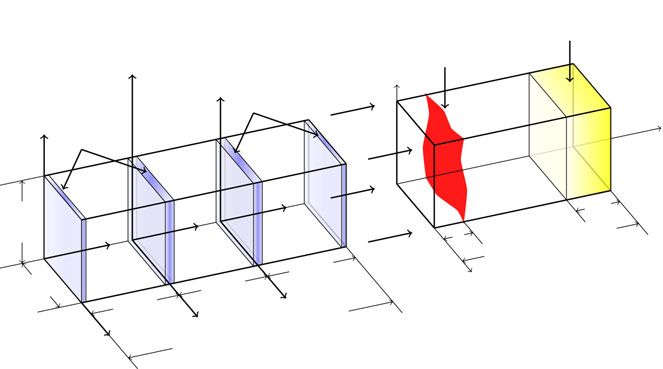
Downloaded from https://www.cambridge.org/core. IP address: 46.4.80.155, on 06 Nov 2020 at 08:03:04, subject to the Cambridge Core terms of use, available at https://www.cambridge.org/core/terms. https://doi.org/10.1017/jfm.2020.292
Parametric numerical study of passive scalar mixing in STI 895 A21-3
do not present amplification across the shock but a monotonic decay. Lower fidelity
simulation approaches, such as large-eddy simulations (LES) (Bermejo-Moreno,
Larsson & Lele 2010; Hickel, Egerer & Larsson 2014; Braun, Pullin & Meiron 2019)
and Reynolds (or Favre) averaged Navier–Stokes (RANS) simulations (Sinha, Mahesh
& Candler 2003; Quadros & Sinha 2016; Schwarzkopf et al. 2016) have emerged in
the last two decades.
Studies of scalar mixing in the canonical STI configuration are scarce in comparison
with other compressible flow configurations, such as compressible homogeneous
isotropic turbulence (Pan & Scannapieco 2010, 2011; Ni 2015, 2016; Danish, Suman
& Girimaji 2016) and the shock-driven Richtmyer–Meshkov instability (Brouillette
2002; Lombardini, Pullin & Meiron 2012; Orlicz et al. 2015; Desjardins et al. 2018;
Reese et al. 2018). Tian et al. (2017) analysed the effects of density variations on
STI and mixing by comparing single- and two-fluid cases using shock-capturing DNS.
Faster increase of turbulence stretching and an increased scalar dissipation rate across
the shock were identified as the causes for better mixing enhancement for multi-fluid
mixing. Boukharfane, Bouali & Mura (2018) compared the streamwise evolution of
scalar variance and its dissipation rate between the shocked and unshocked cases, and
observed an increase of scalar dissipation rate (SDR) across the shock. They also
related the increase of SDR with the change of alignments across the shock. These
pioneering studies of scalar mixing in STI were however limited in the Reynolds
number as well as shock and turbulence Mach numbers of the interactions considered,
which were all in the wrinkled-shock regime. Besides the limited number of studies
on scalar mixing under STI, other works have investigated compressibility effects
on mixing (Pantano & Sarkar 2002; Vaghefi & Madnia 2015; Karimi & Girimaji
2016; Jahanbakhshi & Madnia 2016; Arun et al. 2019; Yu & Lu 2019). Although
not focused on passive scalars, these investigations have identified flow patterns that
are favoured and dominate dissipation in locally compressed regions, relevant to STI.
Building upon Larsson et al. (2013) and Gao et al. (2018), our present work
uses shock-capturing DNS to study passive scalar mixing in the canonical STI
configuration under a wider range of physical parameters than previously explored.
Wrinkled- and broken-shock regimes are considered for different mean and turbulence
Mach numbers, Reynolds number and Schmidt number. The objective is to elucidate,
through parametric studies, the streamwise evolution across the shock wave and in
the downstream relaxation region of dominant scalar mixing quantities in relation to
changes of the background turbulence. The datasets generated from these simulations,
including full volumetric fields as well as processed data, are available for download
from the corresponding authors.
2. Methodology
2.1. Numerical setup, governing equations and numerical scheme
Shock-capturing direct numerical simulations are used to solve the conservative form
of the equations of mass, momentum and total energy conservation of a Newtonian,
calorically perfect gas, complemented with transport equations for passive scalars:
∂t ρ + ∂j (ρuj ) = 0, (2.1)
∂t ρui + ∂j (ρuj ui ) = ∂j σij , (2.2)
∂t (ρeT ) + ∂j (ρuj eT ) = ∂j (ui σij ) − ∂j qj , (2.3)
∂t ρφα + ∂j (ρuj φα ) = ∂j (ρDα ∂j φα ). (2.4)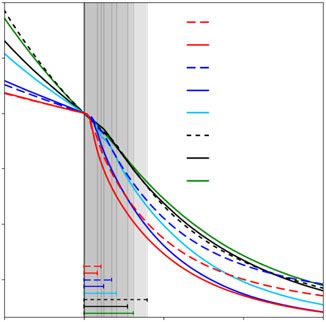
Downloaded from https://www.cambridge.org/core. IP address: 46.4.80.155, on 06 Nov 2020 at 08:03:04, subject to the Cambridge Core terms of use, available at https://www.cambridge.org/core/terms. https://doi.org/10.1017/jfm.2020.292
895 A21-4 X. Gao, I. Bermejo-Moreno and J. Larsson
Case Reλ ReL M Mt L /η Resolution Regime Line style Symbol
2
A 41 213 1.28 0.31 65 1280 × 384 Broken —— (green) E (green)
B 37 177 1.5 0.09 56 1700 × 5122 Wrinkled ······ B
C 38 191 1.5 0.20 60 1280 × 3842 Wrinkled –-–-– D
D 39 193 1.5 0.31 60 1280 × 3842 Wrinkled —— @
E 40 201 1.5 0.42 62 1280 × 3842 Broken ––– E
F 38 177 2.0 0.30 57 1700 × 5122 Wrinkled —— (cyan) E (cyan)
G 37 191 3.0 0.30 60 1280 × 3842 Wrinkled —— (blue) E (blue)
H 37 204 5.0 0.31 63 1280 × 3842 Wrinkled —— (red) E (red)
I 74 679 1.5 0.42 154 2400 × 10242 Broken —— A
J 66 548 3.0 0.29 132 2400 × 10242 Wrinkled — — (blue) A (blue)
K 72 655 5.0 0.31 151 2400 × 10242 Wrinkled — — (red) A (red)
TABLE 1. Simulation cases, line styles and symbols (for postshock state) used in figures.
Here Einstein summation convention is used for Roman subscripts, ∂t = ∂/∂t, ∂j =
∂/∂xj , ρ is the density, ui is the ith component of the velocity (i = 1, 2, 3), eT =
e + 21 ui ui is the total energy per unit mass (e = cv T is the internal energy per unit mass,
cv is the specific heat capacity at constant volume and T is the temperature), and φα is
the αth passive scalar (α = 1, . . . , M). Fourier’s law is used to express the conduction
heat flux as qj = −κ∂j T, where κ is the thermal conductivity, chosen such that the
Prandtl number Pr = cp µ/κ equals 0.7, with cp the specific heat capacity at constant
pressure. The stress tensor is defined as σij = −pδij + τij , where p is thermodynamic
pressure, τij = 2µ(S ij − S kk δij /3) is the viscous stress tensor, S ij = 12 (∂j ui + ∂i uj ) is the
strain-rate tensor and µ is the dynamic viscosity, which follows the power law µ =
µref (T/Tref )3/4 , with reference viscosity and temperature, µref and Tref , respectively. A
zero volumetric viscosity has been assumed. The ideal gas law, p = ρRT, is used to
relate static thermodynamic variables in terms of the gas constant, R.
Reynolds and Favre averages of any flow quantity, f , are denoted by f̄ and ef =
ρf /ρ, respectively, with corresponding fluctuations defined as f 0 = f − f and f 00 = f − ef .
Averaging is done spatially over the statistically homogeneous transverse directions
(y = x2 and z = x3 ) and temporally, since the flow becomes statistically stationary after
an initial transient, by adequately setting the outflow back pressure.
The relevant dimensionless parameters of STI are the mean flow √ (or shockwave)
Mach number, M = e u1,u /ec, the turbulence Mach number, Mt = 3u0rms /ec, and the
Taylor microscale Reynolds number, Reλ = ρ̄u0rms λ/µ̄, where λ = [u02 u02 /(∂2 u2 )2 ]1/2 is
the Taylor microscale, u0rms = (u0i u0i /3)1/2 is the r.m.s. velocity fluctuation and c is
the local speed of sound. Another Reynolds number is considered, ReL = ρu0rms L/µ,
based on the dissipation-based length scale characterizing large eddies, L = K 3/2 /,
i ui /2 is the specific TKE and = τij S ij /ρ its rate of dissipation. Values
00 00
where K = ug
of these dimensionless parameters reported in this work (see table 1) are determined
immediately upstream of the unsteady shock region of each STI simulation. Diffusion
of each passive scalar is characterized by the Schmidt number, Scα = ρDα /µ, assumed
constant in each simulation.
The computational domain for all STI simulations is a rectangular box of size
(Lx , Ly , Lz ) = (4π × 2π × 2π) (see figure 1). The governing equations are discretized
on rectilinear, Cartesian grids, uniformly spaced in the transverse directions, and
stretched in the mean streamwise direction (x = x1 ) to increase the resolution near the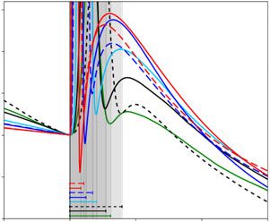
Downloaded from https://www.cambridge.org/core. IP address: 46.4.80.155, on 06 Nov 2020 at 08:03:04, subject to the Cambridge Core terms of use, available at https://www.cambridge.org/core/terms. https://doi.org/10.1017/jfm.2020.292
Parametric numerical study of passive scalar mixing in STI 895 A21-5
Sponge layer
Shock
x wave
z2 ¡ y
Blended
region
Blended z3 ¡ y Inf low
z1 ¡ z region x
HIT 3
HIT 2
HIT 1
z π
2π x3 ¡
y 2 doma
in
x2 ¡ TI
x1 ¡
x 4π, S
2π z
2π 2π x
y3 ¡
2π z
y2 ¡
y atabas
e
y1 ¡ f low d
HIT in
F IGURE 1. Problem setup of STI and blended homogeneous isotropic turbulence (HIT)
precursor simulations.
average shock location. For all simulation cases, 1x2,3 /1x1,s = 2.4, where 1x2,3 is
the grid spacing in the transverse (y and z) directions, and 1x1,s is the grid spacing
in the streamwise direction immediately after the shock.
A solution-adaptive numerical method is employed (Larsson & Lele 2009) that
combines a fifth-order weighted essentially non-oscillatory (WENO) scheme with
HLL flux splitting near shocks, and a sixth-order central difference scheme in the
split form of Ducros et al. (2000) elsewhere. Near-shock regions where WENO is
applied are identified as satisfying −θ > 1.2ωk ωk , where θ = Skk = ∂k uk is the dilatation,
ωk ωk is the enstrophy and ωi = ijk ∂j uk is the vorticity. The equations are advanced
in time using a fourth-order, four-stage explicit Runge–Kutta scheme. Inflow and
outflow boundaries along the streamwise direction use summation by parts operators
with simultaneous approximation terms (Svärd & Nordström 2014). A sponge layer is
used in the STI simulations for x ∈ [xsp , xmax ] = [3π, 4π] to effectively damp acoustic
reflections generated at the outflow boundary, preventing upstream propagation into
the subsonic region of the domain. To obtain a statistically stationary shock, the
back pressure at the outflow plane, pb , is specified following Larsson & Lele (2009).
Periodic boundary conditions are imposed in the transverse directions.
Precursor simulations of decaying homogeneous isotropic turbulence (DHIT) with
transport of passive scalars are performed in a periodic box of size (2π)3 . These
precursor simulations provide turbulence databases that will be superimposed at the
inflow plane of the STI simulations to the mean advection velocity by means of
Taylor’s hypothesis. The uniform, isotropic grid spacing in each DHIT simulation
is dictated by the transverse resolution of the corresponding STI simulation that
will use the inflow dataset. Decaying homogeneous isotropic turbulence simulations
follow Larsson et al. (2013), extended to include passive scalars with initial spectra
E(k) ∝ k4 e−2k /k0 and k0 = 4. The resulting initial passive scalar fields have zero mean
2 2
and unitary variance. Decaying homogeneous isotropic turbulence simulations are run
until reaching the targeted Mt and Reλ , accounting for decay in the STI upstream
of the unsteady shock region. The turbulence is assumed fully developed once the
velocity derivative skewness stabilizes around −0.5 and the dissipation-based length
scale, L , increases with time.
Downloaded from https://www.cambridge.org/core. IP address: 46.4.80.155, on 06 Nov 2020 at 08:03:04, subject to the Cambridge Core terms of use, available at https://www.cambridge.org/core/terms. https://doi.org/10.1017/jfm.2020.292
895 A21-6 X. Gao, I. Bermejo-Moreno and J. Larsson
To obtain an inflow database sufficiently long to allow for the computation of
statistically converged time averages in the STI simulation, snapshots from multiple
realizations of DHIT with the same physical parameters (Mt , Reλ and Scα ) but
different initial conditions are blended following Larsson (2009). In addition, from
each DHIT snapshot (box), two additional boxes, obtained by a series of rotations,
are subsequently blended.
2.2. Simulation cases
In table 1 we present a summary of the simulations performed in this study, varying
Reλ between ≈40 (cases A–H) and ≈70 (I–K), M from 1.28 to 5.0, and Mt from
0.09 to 0.42, which covers a wider parameter space than previously investigated (Tian
et al. 2017; Boukharfane et al. 2018). Wrinkled- and broken-shock regimes are thus
considered in these simulations, according to the criterion that Mt /(M − 1) ' 0.6
is required for the broken-shock regime (see Donzis 2012b; Larsson et al. 2013).
Simulation cases A–H include passive scalars with Sc = 0.5, 1 and 2, whereas cases
I–K consider Sc = 1 only.
After an initial transient that accounts for adjustments to the back pressure to
obtain a statistically stationary state, statistics are collected over a time period
Linput /e
u1,u , or k0e
u1,u tstats = 24π in dimensionless form. Cases B and F, along
with other coarser-resolution simulations not shown in table 1, are used for
grid-convergence analyses described in the supplementary material available at
https://doi.org/10.1017/jfm.2020.292. Simulations with a resolution of 1280 × 384 ×
384 (2400 × 1024 × 1024) are already grid converged for Reλ ≈ 40 (70). At this
resolution, kmax ηB,d > 1.1, where ηB,d is the Batchelor scale immediately downstream
of the shock, for the three values of Sc considered. For all simulation cases, once the
statistically stationary state is reached, the average shock is located k0 1x ≈ 8 behind
the inflow boundary, where the grid resolution is highest.
3. Shock-normal statistics
In this section we focus on the streamwise evolution of scalar mixing statistics
averaged on transverse planes and in time. To compare results from different
simulations in the figures to follow, for each case: (1) the streamwise origin is
shifted to the start of the unsteady shock region; (2) the streamwise coordinate is
rescaled by the dissipation-based length scale taken immediately upstream of the
unsteady shock region, L,u ; (3) the unsteady shock region is either highlighted by a
grey shade and a horizontal line segment marking its width, or removed for better
comparison of the effective jumps of flow quantities across the averaged unsteady
shock regions; (4) when the unsteady shock regions are removed, symbols mark the
postshock location for each case, following table 1.
3.1. Reynolds stress, vorticity variance anisotropy and relevant streamwise locations
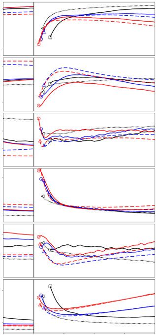
In figure 2(a,b) we show averaged profiles of streamwise Reynolds stresses, Rxx = uf 002 .
For each simulation case, Rxx first peaks in the region of shock unsteadiness, generally
followed by a second peak farther downstream (outside the unsteady shock region)
that results from an acoustic-to-vortical energy transfer (Lee et al. 1993; Larsson
& Lele 2009). We define the averaged preshock, xpre , and postshock, xpost , locations
of each simulation by the first two local minima found in the streamwise profile
of Rxx , respectively. The unsteady shock region lies in between these preshock and
Downloaded from https://www.cambridge.org/core. IP address: 46.4.80.155, on 06 Nov 2020 at 08:03:04, subject to the Cambridge Core terms of use, available at https://www.cambridge.org/core/terms. https://doi.org/10.1017/jfm.2020.292
Parametric numerical study of passive scalar mixing in STI 895 A21-7
(a) 1.75 (b)
1.4
1.50 1.2
¡ ¡
¡ ¡
1.25 1.0
u2/uu2
u2/uu2
1.00 0.8
0.6
0.75
0.4
0.50
-1 0 1 2 3 0 2 4
(c) (d) 3.0
101 K(5.0, 0.3, 72) I(1.5, 0.4, 74)
H(5.0, 0.3, 37) E(1.5, 0.4, 40)
J(3.0, 0.3, 66) 2.5 D(1.5, 0.3, 39)
G(3.0, 0.3, 37) C(1.5, 0.2, 38)
¡ ¡
¡ ¡
øy2/øx2
F(2.0, 0.3, 38)
øy2/øx2 2.0
B(1.5, 0.1, 37)
D(1.5, 0.3, 39)
A(1.28, 0.3, 41)
1.5
100 1.0
0 1 2 3 0 2 4
x/L´,u x/L´,u
F IGURE 2. Streamwise profiles of Favre-averaged streamwise Reynolds stresses (a,b) and
vorticity variance anisotropy (c,d) for different simulation cases. Each curve in (a,b) has
been normalized by the value immediately upstream of the unsteady shock region. Grey
shaded regions and horizontal line segments in (a,b) mark the extent of the unsteady shock
region for each case, using the corresponding line style. All unsteady shock regions are
removed in (c,d) for a clearer comparison among cases. Vertical segments starting from
the horizontal axis indicate the location of xω̂x . M, Mt and Reλ values for each case are
given in parentheses in the legend following table 1.
postshock locations, as marked by the greyed areas and the horizontal line segments in
figure 2(a,b). The width of the unsteady region decreases with M, and increases with
Mt and Reλ . The peak of Rxx downstream of the shock increases in magnitude with M,
tending toward saturation for M > 3, and decreases with Reλ and Mt , which also bring
it closer to the shock. For case I, with (M, Mt , Reλ ) = (1.5, 0.4, 74), the unsteady
shock region is the widest and encloses the region of acoustic-to-vortical energy
transfer, such that there is no local minimum of Rxx immediately downstream of the
shock. The postshock location for this case I is defined instead by the discontinuous
change in slope of Rxx (figure 2b).
The streamwise location downstream of the shock where the streamwise vorticity
variance reaches its maximum is denoted by xω̂x . We define the location of recovery of
small-scale isotropy, xiso , at the streamwise location downstream of the shock where
the vorticity variance anisotropy, ωf y /ωx , recovers to a value of 1.01 (figure 2c,d).
002 f
002
Note that the small-scale anisotropy is highest immediately downstream of the shock,
increasing for larger M, and smaller Mt and Reλ . In contrast with Rxx , the anisotropy
Downloaded from https://www.cambridge.org/core. IP address: 46.4.80.155, on 06 Nov 2020 at 08:03:04, subject to the Cambridge Core terms of use, available at https://www.cambridge.org/core/terms. https://doi.org/10.1017/jfm.2020.292
895 A21-8 X. Gao, I. Bermejo-Moreno and J. Larsson
(a) 1.50 (b)
K(5.0, 0.3, 72) I(1.5, 0.4, 74)
H(5.0, 0.3, 37) E(1.5, 0.4, 40)
1.25
J(3.0, 0.3, 66) D(1.5, 0.3, 39)
G(3.0, 0.3, 37) C(1.5, 0.2, 38)
1.00 F(2.0, 0.3, 38) B(1.5, 0.1, 37)
E(1.5, 0.4, 40)
¡ ¡
ƒ 2/ƒu2
D(1.5, 0.3, 39)
0.75
A(1.28, 0.3, 41)
0.50
0.25
-1 0 1 2 3 -1 0 1 2 3
x/L´,u x/L´,u
F IGURE 3. Streamwise profiles of Favre-averaged scalar variance for (a) cases with the
same Mt and (b) cases with the same M. Sc = 1. Each curve is normalized by the value
immediately upstream of the unsteady shock region, which is greyed out and marked, for
each case, by a horizontal segment with the same line style as the corresponding curve.
does not saturate for the range of M considered here. Higher Reλ leads to a faster
recovery of small-scale isotropy.
3.2. Scalar variance
Whereas there is no local jump of passive scalar variance across the instantaneous
shock, averaging results into an effective jump across the unsteady shock region due
to its finite width (figure 3). The effective jump is defined as the difference between
the xpost and xpre values. The Mach number M has a nearly negligible influence
on this effective jump of scalar variance, as the reduced unsteady shock width is
balanced by a steeper decay rate across the shock. The latter, evidenced by the
increased negative slope of the profiles, results from a larger scalar dissipation rate
(see § 3.3) and a smaller mean velocity downstream of the shock. Larger Mt increases
shock corrugation, widens the unsteady shock region, and produces a larger effective
jump of scalar variance across the shock. Larger Reλ slows down the decay rate of
normalized scalar variance downstream of the shock, a consequence of the reduced
jump of scalar dissipation rate that will be shown in § 3.3.
3.3. Scalar variance budgets
The transport equation for the Favre-averaged passive scalar variance, φ] 00 φ 00 , is
∂t ρ φ]
00 φ 00 + e
ui ∂i ρ φ]00 φ 00 = − ρφ 00 φ 00 ∂ie
ui − 2ρu00i φ 00 ∂i φe − ∂i ρu00i φ 00 φ 00
| {z } | {z } | {z }
A
| {z } B
L1 C
+ 2∂i ρDφ 00 ∂i φ − 2ρD (∂i φ 00 )2 − 2ρD (∂i φ 00 ) ∂i φe,
| {z } | {z } | {z }
D E F
(3.1)
Downloaded from https://www.cambridge.org/core. IP address: 46.4.80.155, on 06 Nov 2020 at 08:03:04, subject to the Cambridge Core terms of use, available at https://www.cambridge.org/core/terms. https://doi.org/10.1017/jfm.2020.292
Parametric numerical study of passive scalar mixing in STI 895 A21-9
where D is the diffusivity of scalar φ. The local time derivative vanishes once
statistical stationarity is reached. The right-hand side includes the dilatational term,
A, proportional to the dilatation of the Favre-averaged mean velocity; production
term, B , proportional to the Favre-averaged mean scalar gradient; turbulent diffusion
term, C ; molecular diffusion term, D; (turbulent) scalar variance dissipation rate
terms, E and F . For all cases considered, terms B , D and F have a negligible
contribution outside the unsteady shock region, and are not shown. The convection of
scalar variance by Favre-averaged mean velocity (L1) and the dilatational term (A)
can be combined into a conservative (divergence-like) flux term for scalar variance.
Thus, the integral of the remaining terms on the right-hand side (C and E ) between
two streamwise locations then equals the change of scalar variance multiplied by the
streamwise momentum.
In figure 4 we show streamwise profiles of the dilatational term A, the turbulent
diffusion term C and the scalar dissipation rate term E . The latter dominates, in
agreement with Tian et al. (2017), while all three terms increase across the shock.
Tian et al. (2017) did not perform a parametric study of different terms in (3.1),
while Boukharfane et al. (2018) only studied the effects of M (for 1.7, 2.0 and 2.3)
on the scalar dissipation term. Dilatational and turbulent diffusion terms reach about
ten percent of the scalar dissipation rate term downstream of the shock, in contrast
to the results of Tian et al. (2017), who found these two terms to be negligible for
the mixing of passive scalars, but not for multi-fluid mixing. Our present simulations
predict the dilatational and turbulent diffusion terms to be also significant in the
mixing of passive scalars, more so for larger M and smaller Reλ . Boukharfane
et al. (2018) also observed a non-negligible turbulent diffusion term. The dilatational
term peaks shortly downstream of the unsteady shock region. The normalized peak
increases with M for M 6 3 and slightly decreases for larger M. Downstream of the
shock, a rapid decay of the dilatational and turbulent diffusion terms follows along
a streamwise distance shorter than L,u . The two terms become slightly negative and
recover to negligible values approximately 3L,u behind the shock. For increasing Mt ,
the peak of initial decay is embedded in the wider unsteady shock region (e.g. case
I in the broken-shock regime).
The effective jump of scalar dissipation rate E across the shock monotonically
increases with M (in agreement with Boukharfane et al. (2018)), and decreases with
Mt and Reλ , showing no sign of saturation up to M = 5. Larger Reλ results in a
lower effective jump of scalar dissipation across the shock. To decouple the effect
of increased density and viscosity across the shock for cases with different M, we
introduce a scaled scalar dissipation, χ̂ = E /2ρD = ρD(∂i φ 00 )2 /ρD. This quantity,
plotted in figure 5, also shows increasing jump with M across the unsteady shock
region, with no signs of saturation. A faster downstream decay is also observed as
M increases, whereas larger Reλ mainly lowers the postshock value. The wider shock
region brought in by increased Mt leads to effective jumps of χ̂ /χ̂u below unity for
cases in the broken-shock regime. It is expected that as Mt is further increased,
possibly entering the ‘vanished (shock) regime’, amplification of scalar-related
quantities will be progressively reduced, eventually leading to a decay across the
shock, as seen for turbulence quantities in Chen & Donzis (2019).
3.4. Scalar Taylor-like microscale
In figure 6 we show the influence of M, Mt and Reλ on the scalar Taylor-like
microscale, defined as λφ = (φ]00 φ 00 /χ̂)1/2 . Across the shock, λ decreases, more so for
φ
Downloaded from https://www.cambridge.org/core. IP address: 46.4.80.155, on 06 Nov 2020 at 08:03:04, subject to the Cambridge Core terms of use, available at https://www.cambridge.org/core/terms. https://doi.org/10.1017/jfm.2020.292
895 A21-10 X. Gao, I. Bermejo-Moreno and J. Larsson
(a) (b) 0.2
K(5.0, 0.3, 72) I(1.5, 0.4, 74)
0.3 H(5.0, 0.3, 37) E(1.5, 0.4, 40)
J(3.0, 0.3, 66) D(1.5, 0.3, 39)
G(3.0, 0.3, 37) 0.1 C(1.5, 0.2, 38)
0.2
a/eu
F(2.0, 0.3, 38) B(1.5, 0.1, 37)
D(1.5, 0.3, 39)
0.1 A(1.28, 0.3, 41)
0
0
-0.1
(c) (d) 0.10
0.3
0.05
0.2
c/eu
0
0.1
-0.05
0
-0.1 -0.10
(e) 15.0 (f)
2.0
12.5
10.0 1.5
e/eu
7.5
1.0
5.0
0.5
2.5
0 0
0 1 2 3 0 1 2 3
x/L´,u x/L´,u
F IGURE 4. Streamwise profiles of non-negligible terms in the transport equation of scalar
variance for cases with the same Mt (a,c,e) and cases with the same M (b,d,f ). Each curve
is normalized by the value immediately upstream of the unsteady shock region (removed
for clarity). The preshock location is offset to be at x = 0 for all cases, and the postshock
location, xpost , is marked with symbols, (a,b) dilatational term; (c,d) turbulent diffusion
term; (e,f ) dissipation rate of scalar variance.
increasing M and decreasing Reλ . Downstream of the unsteady shock region, λφ grows
at a rate that increases with M and Reλ . Cases with relatively low M (1.28 and 1.5)
show a monotonic growth rate, with a nearly uniform λφ for downstream distances
below approximately L,u . Cases with larger M (≈2–5) show a non-monotonic growth
rate, with a fast growth very close to the unsteady shock region (x < L,u /3), followed
by a slowdown and a subsequent acceleration. Cases in the wrinkled-shock regime
share a similar effective jump and downstream recovery of the normalized λφ , whereasDownloaded from https://www.cambridge.org/core. IP address: 46.4.80.155, on 06 Nov 2020 at 08:03:04, subject to the Cambridge Core terms of use, available at https://www.cambridge.org/core/terms. https://doi.org/10.1017/jfm.2020.292
Parametric numerical study of passive scalar mixing in STI 895 A21-11
(a) ç^/ç^u (b) ç^/ç^u
2.0
4
3 1.5
2 1.0
1 0.5
0 0
0 1 2 3 0 1 2 3
x/L´,u x/L´,u
F IGURE 5. Streamwise profiles of scaled scalar dissipation rate, χ̂, for (a) cases with
the same Mt and (b) cases with the same M. Each curve is normalized by the value
immediately upstream of the unsteady shock region (removed for clarity). Symbols mark
the postshock location, xpost . Legend as in figure 4.
(a) ¬ƒ/¬ƒ,u (b) ¬ƒ/¬ƒ,u
1.0 1.2
0.8 1.0
0.6
0.8
0.4
0 1 2 3 0 1 2 3
x/L´,u x/L´,u
F IGURE 6. Streamwise profiles of scalar Taylor-like microscale, λφ = (φ]
00 φ 00 /χ̂)1/2 , for
(a) cases with the same Mt and (b) cases with the same M. Each curve is normalized
by the value immediately upstream of the unsteady shock region. Legend as in figure 4.
the widened unsteady shock region for cases in the broken-shock regime results in
smaller effective jump and faster downstream recovery.
3.5. Effect of Schmidt number
The effect of the Schmidt number, Sc, is examined in figure 7, which shows
streamwise profiles of scalar variance and dissipation for three Schmidt numbers
(Sc = 0.5, 1 and 2) extracted from simulation case H. In this range, Sc has a negligible
effect on the scalar variance normalized by its corresponding value immediately
upstream of the shock. A small difference is seen in the jump of normalized
scalar dissipation across the unsteady shock region, slightly larger in magnitude
for increasing Sc, that persists downstream in the otherwise similar evolution of
scalar dissipation for all Sc. Likewise, Sc was found to have a negligible effect on
other scalar quantities (not shown) including other terms in the transport equations
of scalar variance and dissipation, on the dissipation conditioned by flow topology,
and on the alignment of the scalar gradient with vorticity and strain-rate tensor
eigenvectors, to be discussed later. Similar conclusions regarding the effect of ScDownloaded from https://www.cambridge.org/core. IP address: 46.4.80.155, on 06 Nov 2020 at 08:03:04, subject to the Cambridge Core terms of use, available at https://www.cambridge.org/core/terms. https://doi.org/10.1017/jfm.2020.292
895 A21-12 X. Gao, I. Bermejo-Moreno and J. Larsson
(a) ¡ ¡ (b)
ƒ 2/ƒu2 ç^/ç^u
1.00 Sc = 2.0
Sc = 1.0
0.75 Sc = 0.5 4
0.50
2
0.25
0 0
0 1 2 3 0 1 2 3
x/L´,u x/L´,u
F IGURE 7. Streamwise profiles of (a) Favre-averaged scalar variance and (b) its scaled
rate of dissipation for scalars with different Sc obtained from case H (M = 5.0, Mt = 0.3,
Reλ = 37). Each curve is normalized by the value immediately upstream of the unsteady
shock region, shaded in grey.
apply to other simulations cases, including wrinkled- and broken-shock regimes. In
what follows, only results for Sc = 1 will be considered, and the effects of the other
dimensionless numbers (M, Mt and Reλ ) will be studied in detail.
3.6. Scalar dissipation budgets
The Reynolds-averaged transport equation for the scalar dissipation, χ = (∂i φ)2 , can
be expressed as
∂t χ + uk ∂k χ = − u0k ∂k χ − 2(∂i uk )(∂i φ)(∂k φ) + 2(∂i φ)∂i [ρ −1 ∂k (ρD∂k φ)] . (3.2)
| {z } | {z } | {z } | {z }
L2 G H I
Budgets of scalar dissipation were previously analysed in compressible DHIT (Danish
et al. 2016, e.g.), but the shock-normal evolution of these terms under STI has not
been reported to date. As in the transport equation for scalar variance, the local
time derivative on the left-hand side vanishes in the statistically stationary regime.
The convection of scalar variance by the Reynolds-averaged mean velocity is then
balanced by the terms on the right-hand side. The first term, G , represents the
correlation between Reynolds velocity fluctuations and the gradient of the scalar
dissipation. The second term, H, results from the interaction of spatial gradients
of the velocity and passive scalar fields. Alignment of the scalar gradient with the
eigenvectors of the velocity gradient tensor thus plays a key role in the amplification
or reduction of scalar dissipation and in the overall mixing (see §§ 4 and 5). The last
term, I , accounts for molecular diffusion processes.
In figure 8 we compare the contribution of G , H and I for all simulated cases.
Each profile is normalized with the preshock magnitude of the molecular diffusion
term, |Iu |. The velocity-scalar interaction term has a net positive contribution
(i.e. amplification of dissipation, hence leading to better mixing), whereas the
molecular diffusion term has a net negative contribution to the right-hand side
equation (3.2), contributing to the ‘production’ and ‘destruction’ of scalar dissipation,
respectively.Downloaded from https://www.cambridge.org/core. IP address: 46.4.80.155, on 06 Nov 2020 at 08:03:04, subject to the Cambridge Core terms of use, available at https://www.cambridge.org/core/terms. https://doi.org/10.1017/jfm.2020.292
Parametric numerical study of passive scalar mixing in STI 895 A21-13
(a) (b) 2.0
K(5.0, 0.3, 72)
4
H(5.0, 0.3, 37)
1.5
J(3.0, 0.3, 66)
3 G(3.0, 0.3, 37)
-h/|iu|
F(2.0, 0.3, 38) 1.0
D(1.5, 0.3, 39)
2 I(1.5, 0.4, 74)
A(1.28, 0.3, 41) 0.5
E(1.5, 0.4, 40)
D(1.5, 0.3, 39)
1 0 C(1.5, 0.2, 38)
B(1.5, 0.1, 37)
0 -0.5
(c) 12.5 (d) 2.5
-g/|iu|
0.02
10.0 2.0
-i/|iu|
7.5 0.01 1.5
5.0 1.0
0
0 2 4
2.5 0.5
0 0
0 1 2 3 0 1 2 3
x/L´,u x/L´,u
F IGURE 8. Streamwise profiles of right-hand-side terms in the Reynolds-averaged
transport equation for the scaled dissipation of scalar variance for cases with the same
Mt (a,c) and cases with the same M (b,d). (a,b) Interaction between velocity gradient
tensor and scalar gradient, H. (c,d) Molecular diffusion I . The correlation between the
fluctuating velocity and the gradient of dissipation, G , is shown in the inset of (c)
for selected cases, for clarity. Each curve is normalized by Iu , the absolute value of
the molecular diffusion term immediately upstream of the unsteady shock (removed for
clarity). Symbols mark the postshock location, xpost .
Whereas the velocity-scalar-gradient, H, and molecular diffusion, I , terms are of the
same order, the latter is always the largest in magnitude, for all cases and streamwise
locations. The molecular diffusion term shows an effective jump in magnitude across
the shock that is monotonically increasing with larger M, and smaller Mt . The effects
of Reλ are less obvious. The streamwise profiles show a monotonic shallowing of
the slope downstream of the shock. In contrast, the velocity-scalar-gradient interaction
term experiences a jump of magnitude across the shock that appears to saturate for
M ' 3 and increases with larger Reλ and smaller Mt , in the wrinkled-shock regime.
The contribution from the fluctuating-velocity/dissipation-gradient correlation term, G ,
is predominantly positive, but much smaller (below 1 %) than the other two terms. The
term G is only shown for selected cases in the inset, for clarity.
3.7. Spectra and PDFs
Time-averaged spectra of passive scalar calculated on transverse planes, Ěφ , at
preshock and postshock locations are compared in figure 9(a) for different simulationDownloaded from https://www.cambridge.org/core. IP address: 46.4.80.155, on 06 Nov 2020 at 08:03:04, subject to the Cambridge Core terms of use, available at https://www.cambridge.org/core/terms. https://doi.org/10.1017/jfm.2020.292
895 A21-14 X. Gao, I. Bermejo-Moreno and J. Larsson
(a) Eƒ(k) (b) Eƒƒ(k)
101 xpost
Re¬ £ 70
100 xpost
xpre
10-1 -5/3
xpre
E(1.5, 0.4, 40) 10-2 Re¬ £ 40
10-3 G(3, 0.3, 37)
H(5, 0.3, 37) 10-4
10-5 I(1.5, 0.4, 74)
10-7 J(3, 0.3, 63) 10-6
K(5, 0.3, 72)
10-9 10-8
100 101 102 100 101 102
k/k0 k/k0
F IGURE 9. Spectra of (a) passive scalar and (b) scalar variance for different simulation
cases at preshock and postshock locations. Each spectrum is normalized by its integral
over all wavenumbers. Spectra for cases with higher Reλ (≈70) have been shifted up two
decades. Postshock spectra are shifted by a factor of 3 relative to preshock counterparts.
The black straight segment with −5/3 slope marks the extent of the inertial range of
scales for the higher Reλ cases, obtained from spectra of the kinetic energy (not shown).
(a) Eç(k; xpre) (b) Eç(k; xpost) (c) Eç(k; x)/Eç(k; xpre)
Re¬ £ 70 Re¬ £ 70 xpre
10-1 10-1 101 xpost
xø^y
10-2 Re¬ £ 40 10-2 Re¬ £ 40 xiso
E(1.5, 0.4, 40) E(1.5, 0.4, 40)
10-3 G(3, 0.3, 37) 10-3 G(3, 0.3, 37)
H(5, 0.3, 37) H(5, 0.3, 37)
10-4 I(1.5, 0.4, 74) 10-4 I(1.5, 0.4, 74) 100
J(3, 0.3, 63) J(3, 0.3, 63)
10-5 K(5, 0.3, 72) 10-5 K(5, 0.3, 72)
0 1 2
10 10 10 100 101 102 100 101 102
k/k0 k/k0 k/k0
F IGURE 10. Comparison of time-averaged spectra of scalar dissipation on transverse
planes for different simulation cases in the (a) preshock and (b) postshock states. Each
spectrum is normalized to unitary integral. Spectra for cases with higher Reλ (≈70) are
shifted up one decade for clarity. (c) Comparison of spectra of scalar dissipation at
different streamwise locations for case K, where each spectrum in (c) is normalized by
the value at the same wavenumber in the preshock spectrum.
cases. Within the limited inertial range of length scales of the present simulations, the
spectra of kinetic energy (not shown) upstream of the shock exhibit an approximate
Ě(k) ∝ 2/3 k−5/3 scaling, consistent with the prediction of Kolmogorov (1941) for
incompressible HIT. However, the passive scalar spectra in the inertial-convective
range depart from the Ěχ (k) ∝ −1/3 χk−5/3 prediction of Obukhov (1949) and Corrsin
(1951) for passive scalar mixing in incompressible HIT. A slope shallower than −5/3
is observed in the inertial-convective range upstream of the shock for all cases, which
may be attributed to the moderate Reynolds numbers of our simulations, following
Danaila & Antonia (2009). For all cases, the spectral content of passive scalar and
its variance increases across the shock for small scales (figure 9a,b), plausibly a
consequence of the immediate amplification of transverse vorticity.Downloaded from https://www.cambridge.org/core. IP address: 46.4.80.155, on 06 Nov 2020 at 08:03:04, subject to the Cambridge Core terms of use, available at https://www.cambridge.org/core/terms. https://doi.org/10.1017/jfm.2020.292
Parametric numerical study of passive scalar mixing in STI 895 A21-15
(a) 10-1 (b) (c)
10-1
10-3
10-3
10-3
10-5 xpre
10-5 10-5
xpost
10-7 xø^y
10-7 10-7 xiso
-2 0 2 0 0.25 0.50 0.75 1.00 0 2 4 6
ƒ log(1 + ƒƒ) log(1 + ç)
F IGURE 11. Probability density functions of (a) passive scalar, (b) scalar variance and
(c) scalar dissipation for case K at xpre (dotted), xpost (solid), xω̂x (dashed), xiso (dash–
dotted). The dash–dot–dotted line in (a) corresponds to a Gaussian distribution with zero
mean and the standard deviation of the PDF of passive scalar at xiso .
In contrast, spectra of scalar dissipation, Ěχ , display a shift of spectral content
across the shock from smaller to larger scales for increasing M and lower Reλ
(see figure 10a,b). Taking case K as an example (figure 10c), amplification of
all wavenumbers is first observed in the postshock state (xpost ), predominantly at
very small scales, followed by large and intermediate scales. Between xpost and xω̂x ,
the readjustment of transverse into streamwise vorticity counteracts the postshock
viscous decay at small scales, such that the spectral content of scalar dissipation is
reduced much more significantly at large and intermediate scales than at small scales.
Downstream of xω̂x , viscous decay affects all scales similarly, preserving the shape of
the spectra.
Time-averaged, transverse-plane probability density functions (PDFs) of passive
scalar, its variance and its dissipation for case K at different streamwise locations are
shown in figure 11. Super-Gaussian passive scalar PDFs, indicative of intermittency,
show a monotonic narrowing downstream as the scalar variance decreases, as
previously observed in Tian et al. (2017) and Boukharfane et al. (2018). The
streamwise evolution of PDFs of scalar variance and scalar dissipation (figure 11b,c)
was not reported in those previous studies. PDFs of scalar dissipation shift significantly
across the shock toward larger values, followed downstream by a progressive recovery
to preshock shapes, completed between the streamwise locations of maximum
enstrophy (xω̂x ) and small-scale isotropy recovery (xiso ). Similar observations hold for
other cases (not shown), with higher Reλ resulting in wider tails of scalar dissipation,
consistent with the study of passive scalar mixing in compressible HIT by Ni (2015).
4. Flow topology and conditioned dissipation rate
4.1. Characterization of local flow topology
Deformation, rotation and stretching (hence mixing) of material elements is character-
ized by local flow topologies that relate streamline patterns moving with the fluid
element to the invariants of the velocity gradient tensor by means of critical point
theory (Chong, Perry & Cantwell 1990). Compared with incompressible flows,
compressibility introduces a richer set of topologies and different formulations of
the topology analysis (Pirozzoli & Grasso 2004; Suman & Girimaji 2010; Vaghefi
& Madnia 2015; Parashar, Sinha & Srinivasan 2019). In the present study, following
Suman & Girimaji (2010), we normalize the velocity gradient tensor Aij = ∂i ujDownloaded from https://www.cambridge.org/core. IP address: 46.4.80.155, on 06 Nov 2020 at 08:03:04, subject to the Cambridge Core terms of use, available at https://www.cambridge.org/core/terms. https://doi.org/10.1017/jfm.2020.292
895 A21-16 X. Gao, I. Bermejo-Moreno and J. Larsson
(a) USN3 (b) (c) SSN3
0.1 UFC SFS
UN3 SN3
UFS SFC
0
q SFS UFC
SFS UFC
SNSS UNSS
UNSS SNSS
-0.1
SNSS UNSS
-0.01 0 0.01 -0.01 0 0.01 -0.01 0 0.01
r r r
F IGURE 12. Flow topologies in pqr space mapped onto three representative planes
with (a) p < 0 (extension), (b) p = 0 (volume-preserving) and (c) p > 0 (contraction),
partitioned by the intersections of each plane with the dividing surfaces S1a (dashed),
S1b (dash–dotted), S2 (solid) and the r = 0 plane (dotted): SFS, stable focus
stretching; UFS, unstable focus stretching; SFC, stable focus compressing; UFC, unstable
focus compressing; SNSS, stable-node/saddle/saddle; UNSS, unstable-node/saddle/saddle;
SN3 , stable node/stable-node/stable-node; UN3 , unstable-node/unstable-node/unstable-node;
SSN3 , stable-star-node/stable-star-node/stable-star-node; USN3 , unstable-star-node/unstable-
star-node/unstable-star-node. The last two topologies correspond to the intersection of S1a
and S1b for p < 0 and p > 0, respectively.
√
as aij = Aij / Apq Apq , from which normalized strain-rate and rotation-rate tensors are
obtained as sij = (aij + aji )/2 and w ij = (aij − aji )/2, respectively. The three invariants of
aij are then expressed as p = −tr(aij ), q = 12 (p2 − sij sji − w ij w ji ) and r = − det(aij ), and
determine the character (real or complex) of the three eigenvalues of Aij , thus defining
the local streamline pattern and flow topology. The pqr space is partitioned into ten
different flow topologies (see figure 12) by the r p = 0 plane and three dividing surfaces,
S1(a, b), defined by (p/3)(q − 2p2 /9) ∓ (2/27) −3q + p2 − r = 0, and S2, defined
by pq = r. Surfaces S1(a, b) separate regions with three real eigenvalues (non-focal
topologies) from regions with one real and two complex conjugate eigenvalues (focal
topologies). Surface S2 contains purely imaginary eigenvalues. Stable (unstable)
topologies indicate that the local streamlines are directed toward (away from) the
critical point.
4.2. One-dimensional PDFs and conditioned scalar dissipation distributions
For each case and streamwise location, E(χ|f ) denotes the distribution of scalar
dissipation, χ, conditioned on the invariant f ∈ (p, q, r). This distribution is
subsequently time-averaged and normalized by the Reynolds-averaged scalar dissipation,
χ, at the same streamwise location, to obtain Ê(χ|f ) = hE(χ|f )i/χ, where h·i
is the time-averaging operator. In figure 13 we show time-averaged PDFs of the
p, q and r invariants, and the corresponding normalized conditional distributions
of scalar dissipation, Ê(χ|p), Ê(χ|q) and Ê(χ|r), extracted at the xpre (preshock),
xpost (postshock) and xiso (return to vorticity-variance isotropy) locations defined in
§ 3.1. Results from only a subset of the simulation cases are plotted for clarity, to
highlight the effect of M, Mt and Reλ .Downloaded from https://www.cambridge.org/core. IP address: 46.4.80.155, on 06 Nov 2020 at 08:03:04, subject to the Cambridge Core terms of use, available at https://www.cambridge.org/core/terms. https://doi.org/10.1017/jfm.2020.292
Parametric numerical study of passive scalar mixing in STI 895 A21-17
(a) xpre (b) xpost (c) xiso
1.2 1.2 1.1
E^(ç|p) E^(ç|p) E^(ç|p)
1.1 1.1 1.0
1.0 1.0
0.9
15 0.9 0.9
0.8
0.8 6 0.8 6
10 0.7
0.7 4 0.7 4
5 PDF(p) PDF(p) PDF(p) 0.6
0.6 2 0.6 2
0 0 0
-0.5 0 0.5 -0.5 0 0.5 -0.5 0 0.5
p p p
(d) 1.50 (e) 1.50 (f) 1.50
1.25 1.25 1.25
E^(ç|q) E^(ç|q) E^(ç|q)
1.00 1.00 1.00
1.5 0.75 0.75 1.5 0.75
2
1.0 0.50 0.50 1.0 0.50
1 0.5
0.5 PDF(q)
0.25 PDF(q)
0.25 PDF(q)
0.25
0 0 0
-0.5 0 0.5 -0.5 0 0.5 -0.5 0 0.5
q q q
(g) 1.2 (h) 1.2 (i) 1.2
E^(ç|r) E^(ç|r) E^(ç|r)
1.0 1.0 1.0
0.8 30 0.8 0.8
10 10
20
PDF(r) PDF(r) PDF(r)
5 0.6 0.6 5 0.6
10
0 0 0
-0.18 0 0.18 -0.18 0 0.18 -0.18 0 0.18
r r r
D(1.5, 0.3, 39) G(3.0, 0.3, 37) H(5.0, 0.3, 37)
E(1.5, 0.4, 40) J(3.0, 0.3, 66) K(5.0, 0.3, 72)
F IGURE 13. Probability density functions of p (a–c), q (d–f ) and r (g–i), along with
normalized distributions of scalar dissipation conditioned on the respective invariant,
extracted at xpre (a,d,g), xpost (b,e,h) and xiso (c,f,i) for cases with different (M, Mt , Reλ ).
Each plot shows the PDFs of the invariant on the bottom curves (left vertical axis), and the
conditioned scalar dissipation distributions, Ê(χ|f ) for f ∈ (p, q, r), on top (right vertical
axis).
Probability density functions of p (figure 13a–c) are nearly symmetric about p =
0 (i.e. incompressible events), where they peak, wider for larger Mt (owing to the
larger velocity fluctuations relative to the sound speed), and narrower for increasingDownloaded from https://www.cambridge.org/core. IP address: 46.4.80.155, on 06 Nov 2020 at 08:03:04, subject to the Cambridge Core terms of use, available at https://www.cambridge.org/core/terms. https://doi.org/10.1017/jfm.2020.292
895 A21-18 X. Gao, I. Bermejo-Moreno and J. Larsson
M and Reλ . At xpost the peak of the p-PDF is nearly half of its preshock magnitude.
Normalized distributions of scalar dissipation conditioned on p, Ê(χ|p), also peak at
p = 0, but are significantly flattened at xpost , as the p-PDFs widen, indicating a more
even distribution of the dissipation across compressible flow topologies compared to
the preshock state. The broken-shock regime simulation shows the largest asymmetry
of Ê(χ|p) at xpre and xpost . By xiso all distributions have widened relative to xpre and
become nearly symmetric.
Preshock q-PDFs (figure 13d–f ) are negatively skewed (i.e. strain-rate dominated),
more so for increasing Reλ . The shape of the q-PDFs is altered at xpost , especially
for larger M, increasing the magnitude of the peak (found at q ≈ 0), which narrows
the core of the distributions. At xiso , the q-PDFs recover the preshock shape, nearly
overlapping for all cases considered. The normalized distributions of scalar dissipation
conditioned on q, Ê(χ|q), are skewed toward q < 0, indicating that scalar dissipation
occurs predominantly in strain-dominated topologies. At xpre and xiso the distributions
nearly collapse for all simulations. However, at xpost , larger M tends to reduce the
skewness, and a local maximum at q ≈ 0 develops. Increasing Reλ counteracts the
effects of a larger M on both the PDF(q) and Ê(χ|q) at xpost .
Probability density functions of r (figure 13g–i) at xpre and xiso are nearly insensitive
to M, Mt and Reλ , and appear skewed toward positive values, corresponding to
predominantly unstable topologies (flow directed away from critical points, whether
rotating or strained), and indicative of the dissipative nature of DHIT. At xpost , higher
M and smaller Reλ narrow and symmetrize the PDFs, which attain larger peaks
at r = 0. A tendency toward symmetrization of the PDF of this third invariant was
observed using LIA and DNS by Ryu & Livescu (2014). The invariant r represents the
competition between the production of kinetic energy dissipation (r > 0) and enstrophy
(r < 0) (see Vaghefi & Madnia 2015; Yu & Lu 2019). Thus, the symmetrization of
the r-PDF indicates a relative increase of enstrophy production across the shock,
and translates farther downstream into a larger scalar dissipation at small scales
(as seen in figure 10c)). The distribution of χ conditioned on r, Ê(χ|r), is largely
skewed toward r > 0 (where production of TKE dissipation prevails) at all streamwise
locations, more so for larger Reλ , peaking at r ≈ 0.1 for xpre and xiso , while flattening
and bringing its peak closer to r = 0 at xpost .
4.3. Joint qr-PDFs and conditioned scalar dissipation distributions
Distinct regions in the qr planes for different values of p define a variety of flow
topologies (figure 12). In figure 14 we show, for case K (M, Mt , Reλ = 5, 0.3, 72),
joint qr-PDFs (contour lines) and conditional χ-distributions (coloured contour map)
at xpre , xpost and xiso for three values of p: negative (extension), zero (incompressible)
and positive (contraction). The teardrop shape commonly found in incompressible
flows is recovered for p = 0 at the three locations. It is observed that χ concentrates
on the right lower tail (q < 0 and r > 0) of the teardrop, below and near the S1b line,
which confirms UNSS as the most dissipative topology at those locations, consistent
with previous findings for compressible and incompressible turbulence (Brethouwer,
Hunt & Nieuwstadt 2003; Danish et al. 2016). Non-zero p values modify the shape
of the qr-PDFs, symmetrizing its outer edge, whereas χ remains largely concentrated
in the UNSS topology. In figure 15 we compare joint qr-PDF and conditioned
χ distributions for p = 0 among the three cases with the higher Reλ (≈70). As M
increases, the qr-PDF preserves the teardrop shape but considerably narrows toward
the origin. Conditional χ distributions still appear predominantly concentrated in the
fourth quadrant for larger M, with the peak moving toward the origin.You can also read