Modelling Population Dynamics of Social Protests in Time and Space: The Reaction-Diffusion Approach - MDPI
←
→
Page content transcription
If your browser does not render page correctly, please read the page content below
mathematics
Article
Modelling Population Dynamics of Social Protests in
Time and Space: The Reaction-Diffusion Approach
Sergei Petrovskii 1,2, *, Weam Alharbi 3 , Abdulqader Alhomairi 4 and Andrew Morozov 1,5
 1   School of Mathematics and Actuarial Science, University of Leicester, Leicester LE1 7RH, UK;
     am379@le.ac.uk
 2   Peoples Friendship University of Russia (RUDN), 6 Miklukho-Maklaya St, Moscow 117198, Russia
 3   Mathematics Department, Faculty of Science, Tabuk University, Tabuk 71491, Saudi Arabia;
     wgalharbi@ut.edu.sa
 4   Department of Curriculum and Teaching Methods, Faculty of Education and Art, Tabuk University,
     Tabuk 71491, Saudi Arabia; ahomari@ut.edu.sa
 5   Institute of Ecology and Evolution, Russian Academy of Sciences, 33 Leninskii pr., Moscow 119071, Russia
 *   Correspondence: sp237@le.ac.uk

 Received: 1 November 2019; Accepted: 20 December 2019; Published: 3 January 2020

 Abstract: Understanding of the dynamics of riots, protests, and social unrest more generally is
 important in order to ensure a stable, sustainable development of various social groups, as well as
 the society as a whole. Mathematical models of social dynamics have been increasingly recognized
 as a powerful research tool to facilitate the progress in this field. However, the question as to what
 should be an adequate mathematical framework to describe the corresponding social processes is
 largely open. In particular, a great majority of the previous studies dealt with non-spatial or spatially
 implicit systems, but the literature dealing with spatial systems remains meagre. Meanwhile, in many
 cases, the dynamics of social protests has a clear spatial aspect. In this paper, we attempt to close this
 gap partially by considering a spatial extension of a few recently developed models of social protests.
 We show that even a straightforward spatial extension immediately bring new dynamical behaviours,
 in particular predicting a new scenario of the protests’ termination.

 Keywords: social dynamics; wave of protests; long transients; ghost attractor

1. Introduction
     Understanding of the dynamics of riots, protests, and social unrest more generally is important in
order to ensure a stable, sustainable development of various social groups, as well as the society as a
whole. To achieve this goal, mathematical modelling has been gaining growing recognition recently
as a powerful research approach [1–14]. Indeed, since replicated sociological experiments with large
groups of people are rarely possible (and it is hardly possible at all to simulate social unrest under
controlled conditions), capturing the complexity of the social dynamics through tractable experiments
is not feasible. Mathematical modelling and computer simulations create a “virtual society” where
hypotheses can be tested and different scenarios investigated in detail, thus providing a feasible
alternative to the experiment.
     A variety of modelling approaches and techniques has been developed and used such as the
costs-benefits analysis [9], social network models [5,10], agent based models [3,7], and behavioural and
epidemiological models [2,11,13,14], both in spatial and non-spatial systems. The models range from
relatively simple, allowing only for some basic feature of the phenomenon [3], to more complicated
ones that take into account more details such as, for instance, heterogeneity of social norms and
behavioural responses [9,15]. The case studies include a few well known events such as the Russian

Mathematics 2020, 8, 78; doi:10.3390/math8010078                           www.mdpi.com/journal/mathematics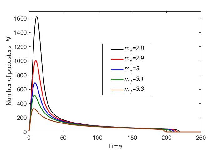
Mathematics 2020, 8, 78                                                                               2 of 19

revolution of 1905–1907 [1], the French riots of 2005 [13], the London riots of 2011 [9], the Arab
Spring [16], and the Yellow Vest Movement in 2018–2019 [17], in particular aiming to describe the
intensity and timing of the unrest and to analyse the processes and mechanisms involved.
      Social protests are known to exhibit a variety of different scenarios. For instance, the total number
of people involved in protests (to which we refer to as “crowd”) can change through time in different
ways, e.g., staying approximately constant for some time and then decaying fast, or decreasing steadily
but slowly. Furthermore, the social structure of the crowd can change significantly, e.g., due to the
individual variability of people’s perception and expectations [18]. Whilst a comprehensive description
of protests requires several state variables and a multivariate analysis (e.g., to account for the individual
variability, cf. [15]), one quantity of immediate importance is the total number of people participating
in the given event at the given time. Arguably, understanding how the total number may evolve
with time provides crucial information needed to ensure security measures and to minimize possible
damage and violence. An inspection of the data on the number of people participating in protests
and riots available for several events of social unrest [9,13,19–21] immediately reveals that there are
some generic properties of the dynamics. There usually exists the main peak, i.e., the maximum in the
participants number (sometimes followed or preceded by secondary peak(s) of smaller magnitude)
followed, in the course of time, by a tail where the number eventually decays to either zero or to
a small background value. However, the rate of decay at the tail can be significantly different for
different events. Whilst in many cases, the number of protesters decays fast, so that the unrest is
effectively over in a matter of weeks [9,13], there have been several cases where the rate of decay is
very slow. One such case is given by the Russian revolution of 1905–1907 [19,20], and another case is
given by the Yellow Vest Movement [21]. As a result of the slow decay in the number of protesters,
the duration of unrest is considerable (about two years for the Russian revolution, about one year
for the Yellow Vest Movement, at the time when this paper was written). A question arises here as
to whether the events with significantly different decay rates are different altogether (e.g., controlled
by different factors) or they are the manifestation of the same social dynamical phenomenon, but
occurring in a different parameter range. A related question is whether it might be possible to develop
a “universal” mathematical model that would embrace the protests with a significantly different decay
rate. Addressing this question is one of the goals of this paper.
      Along with the changes in time, in many cases, riots and protests also have a clear spatial aspect.
For instance, the timing and the intensity of protests can be significantly different at different locations.
Experience gained from studies on dynamical systems of a different origin, e.g., in ecology [22],
indicates that coupling between local protests (e.g., in the context of social dynamics, by the information
exchange and/or spread of ideas) can organize them into a global spatiotemporal pattern. The simplest
example of a spatiotemporal pattern is the travelling wave (sometimes also referred to as the “spreading
wave”). Interestingly, the spreading wave of protests has indeed been observed in some of the events
of social unrest [13,14].
      There is a growing appreciation that the spatial aspect can shape the social protests in a number of
ways; however, most of the previous modelling studies on protests’ dynamics focused on non-spatial
or spatially implicit systems. Apparently, the consensus as to whether an adequate modelling
framework should necessarily be spatial or can be non-spatial has not been reached yet. Whilst
it is well known in other sciences that the dynamical properties of the spatially explicit system often
are significantly different from those of its non-spatial counterpart [22], it remains unclear how the
modelling predictions can differ in the context of the social dynamics. A more specific question is: How
different can the dependence of the protester number on time be in spatial and non-spatial models for
equivalent parameter values? Our paper intends to bridge this gap partially by considering a spatial
extension of two non-spatial models recently developed in [17]. We will show that the dynamics of the
spatial models can be qualitatively different, e.g., predicting the growth in the protester number for the
parameter values where the non-spatial models predict decay. We will also show that the spatial model
brings new dynamical features, in particular predicting a new scenario of the protests’ termination.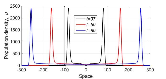
Mathematics 2020, 8, 78                                                                            3 of 19

2. Mathematical Models in the Non-Spatial Case
      We describe the dynamics of protests in terms of average values, hence disregarding any
explicit effects of stochasticity: arguably, this approach works well when applied to sufficiently
large systems [23], i.e., in the context of our study, to sufficiently large groups of people. We assume
that the dynamics can be described by continuous, sufficiently smooth functions of time, so that in the
non-spatial case, the mathematical model consists of ordinary differential equation(s).
      We mention here that any group of people, e.g., the “population” of protesters or the larger
community, is not uniform, but is structured according to various traits [15]. For instance, in the
context of social unrest, the population of protesters can be structured according to the probability for
a given individual to express a violent behaviour. Consider the Yellow Vest Movement as an example:
whilst most participants protested peacefully, there was often a certain fraction that tended to behave
aggressively. The wider community is structured with regard to the probability for a given individual
to join the protests; this, in its turn, correlated with age, income, education, social background, etc.
Whilst some people can be ignited easily (e.g., students [24,25]), people from other social groups might
not so likely join the street actions in any circumstances. Aiming to build tractable models and to
avoid unnecessary complexity (cf. “Occam’s razor”), in this paper, we disregard the effect of individual
differences; in particular, we treat the protesters as a uniform group. We also assume that the total
number of people in the society that could, under certain conditions, join the protests is sufficiently
large and hence is not a factor that limits the growth of the number of protesters.

2.1. Single Species Model
     We describe the civil unrest by a single variable, say N, which is the number of people actively
participating in the street actions [26]. In order to build the model that describes the dynamics of N
with time, we consider the following assumptions:

•     The rate of change in the number of people attending the event is a result of the interplay between
      two processes, recruitment (people joining) and withdrawal (people quitting);
•     Following earlier studies [18], we consider recruitment to be a collective phenomenon so that the
      recruitment rate is a nonlinear function of the number of people currently involved in the event;
•     Decision of withdrawal is made individually, so that the withdrawal rate is a linear function of
      the number of people participating in the event, where the per capita withdrawal rate (say m)
      depends on time.

     Under the above assumptions, we arrive at the following equation for the “population size” of
the demonstrators:
                                   dN (t)
                                          = F ( N ) − m(t) N,                                  (1)
                                     dt
where the first and second terms in the right hand side are the recruitment rate and withdrawal rate,
respectively, and t ≥ 0 is time. We regard the per capita withdrawal rate m as a measure of the
dissatisfaction with the effect of the protests, i.e., when the demands of the demonstrators are not
being met by the authorities. In our model, higher dissatisfaction therefore means a higher rate at
which people quit the movement. In case of an unchanging policy, the dissatisfaction can be expected
to increase with time; hence, m is an increasing function of time.
     We consider the recruitment rate in the following form:

                                                              aN 2
                                      F ( N ) = e0 + eN +            ,                                (2)
                                                            h2 + N 2

where e0 , e, a, and h are nonnegative parameters.
     Parametrization (2) requires further discussion. We first notice that F (0) = e0 ≥ 0. That reflects
the observation that, in almost any society, there is often a fraction of people (albeit normally small)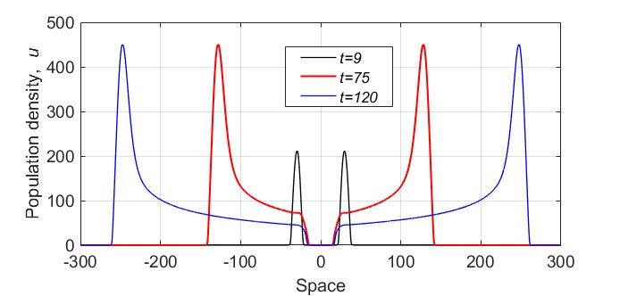
Mathematics 2020, 8, 78                                                                                         4 of 19

who are always ready and willing to rebel, e.g., to join a strike or a civil protest. Such people can be
thought of as zealots that unconditionally support some ideas of ultimate social justice.
    The per capita recruitment rate is given by the following expression:

                                          1          e0       aN
                                            F( N ) =    +e+ 2     .                                                 (3)
                                          N          N     h + N2

       For an intermediate range of N defined by conditions e0 /e  N  h (if parameter values allow
for the existence of such range), the per capita recruitment rate is therefore a monotonously increasing
(approximately linear) function of N. This means that the rate at which new members are joining
the movement tends to increase along with the number of people already in the movement. This is a
typical behaviour response observed not only in humans [27], but also in many animals; in particular,
it is believed to be one of the mechanisms resulting in the Allee effect [28]. However, when the number
of people in the riots becomes large, N  h, the per capita recruitment rate is approximately constant,
 1
 N F ≈ e. That reflects the assumption that there is a certain scale-independent probability of an average
citizen to join protests, which agrees with observations [18,29].
       Before considering the properties of Model (1) and (2) where the withdrawal rate m is a function
of time, it is instructive to start with a simpler case where m is a constant parameter. In this case, it
is readily seen that there exists two critical values, say m∗ and m∗ , so that in an intermediate range
m∗ < m < m∗ , the system possesses three steady states, two of them stable and the third one unstable;
see Figure 1. The system undergoes a saddle-node bifurcation when m passes any of the two critical
values; for m < m∗ and for m > m∗ , there is only one steady state, large population state and small
population state, respectively. In the general case e0 ≥ 0, an analytical expression for m∗ and m∗ is not
available. In a special case e0 = 0, they are given as:
                                                                     √
                                                           ∗             2a − 1
                                       m∗ = e     and    m = e+                 .
                                                                          2h

                                                          Ns

                                                           0
                                                                                m*            m*                m
                           (a)                                                       (b)

      Figure 1. Properties of the model given by Equations (1) and (2) in the baseline case of constant m.
      (a) An example of the relative position of the per capita recruitment rate (black curve) as a function of N
      (in abstract units) and the per capita withdrawal rate (red line). Any intersection between the two lines
      is a steady state. The two stable steady states are shown by the small black circles, and the unstable
      steady state is shown by the red circle. (b) A sketch of the bifurcation diagram: The thick black curve
      shows the steady state value as a function of m. The two long-dashed vertical lines correspond to the
      bifurcation values of m; for any value of m such as m∗ < m < m∗ (see the vertical dotted line), the
      system has three steady states, two stable and one unstable.

      In the case of a variable m, in order to derive the specific expression for m(t), we take into account
that, in the modern society, even in the absence of major events, a number of small scale protests are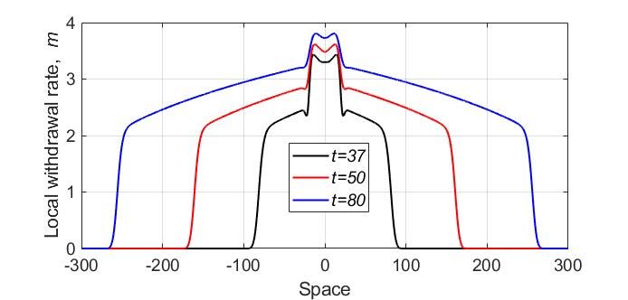
Mathematics 2020, 8, 78 5 of 19
always happening. We assume that there is a certain background rate, say m0 , at which the participants
of those protests quit the actions. We then further assume that the society is in a globally stable state,
so that any perturbation from the background withdrawal rate should decay with time. Trying to
keep the mathematical framework as simple as possible, the simplest equation that describes the
corresponding evolution of m is given as follows:
dm(t)
= b ( m0 − m ), (4)
dt
where b is a coefficient. Equation (4) is readily solved, resulting in:
m(t) = m1 + (m0 − m1 ) 1 − e−bt , (5)
where m1 = m(0) is the initial value of the withdrawal rate. In case the initial value is small, which
can occur as a reflection of high social tensions, m(t) is an increasing function. This seems to be in
agreement with heuristic arguments. Note that, since m has the dimension of inverse time, it can be
written as m = 1/τ where τ is a characteristic duration of the individual participation. In a general
case, τ can change in the course of the protests, hence being a function of time. At the beginning of the
protests, the people’s expectations are high, the morale is high, and people are ready to spend a long
time participating in the event. The characteristic duration of individual involvement is long, and the
initial value of the withdrawal rate m(0) = m1 is small. In the course of the protests, in case there is no
sign of changes, the protesters’ morale may start falling, and the characteristic duration of individual
participation could start decreasing.
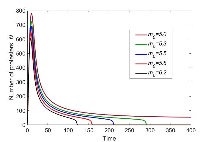
Equations (1) with (2) and (5) are solved numerically. We consider m0 and m1 as the controlling
parameters. Figure 2 shows the solutions obtained for different values of m0 and m1 and other
parameters chosen as e0 = 0.1, e = 3, a = 146, h = 35, and b = 0.01. (We mention here that our choice
of parameter values was not entirely random or hypothetical: it was shown in [17] that, with this
parameter set, Model (1)–(5) provided a good description of the Yellow Vests protests.) We therefore
observe that there are solution properties that are rather robust to parameter variation. In particular,
in all cases shown in Figure 2, the population size creates a peak (which can be rather flat for m1 large
enough; see Curves 5 and 6 in Figure 2b) followed by a gradual decay. This behaviour is in qualitative
agreement with the dynamics of protests often observed in real life. The larger is m0 , the faster the rate
of decay is. For a subcritical value of m0 , i.e., for m0 < m∗ , the population size never falls to the low
background value (which is zero for e0 = 0), but instead stabilizes at a higher positive value (cf. the
magenta curve in Figure 2a), which corresponds to the upper stable steady state of the system; see
the upper black circle in Figure 1b. For a supercritical value m0 > m∗ , the upper steady state does not
exist, so that in the large time limit N eventually converges to its lower steady state value (lower black
circle in Figure 1b). However, if 0 < m0 − m∗
1, the rate of convergence at intermediate time can be
slow because of the “ghost attractor” [30,31]; e.g., see the middle part of the curves in Figure 2b.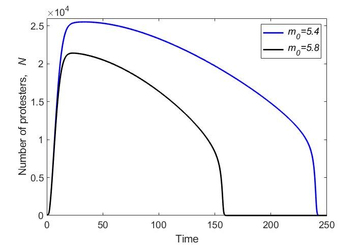
Mathematics 2020, 8, 78                                                                                        6 of 19

                            (a)                                                       (b)

      Figure 2. Solution of Equations (1) with (2) and (5) obtained for different parameter values of m0 and
      m1 . (a) m1 = 3, the values of m0 are given in the figure legend. (b) m0 = 5.5, the values of m1 are given
      in the figure legend. Other parameters are e0 = 0.1, e = 3, a = 150, h = 35, and b = 0.01, which
      corresponds to m∗ = 3.22 and m∗ = 5.15.

2.2. Two Component Model
     In the previous section, the withdrawal rate was described by the self-contained Equation (4)
where the right hand side depends on m only. One weakness of this approach is that it completely
disregards the possible dependence of the right hand side on N. Even in a more general case where
the right hand side in Equation (4) could be a nonlinear function, m is effectively just a given function
of time. As an immediate yet nontrivial extension of the above model, we now consider the case where
the population dynamics of riots is described by the following equations:

                                  dN (t)                         dm(t)
                                         = F ( N ) − mN,               = G (m, N ),                                (6)
                                   dt                             dt
where G is a certain function to be specified.
     Apparently, Model (6) is more general than Model (1) and (2) and hence can describe a broader
variety of situations. In order to find an appropriate parametrization of G, we have to consider more
closely the reasons why people may quit the protests. In doing this, we first observe that street actions
usually bring some economic damage. That can include direct damage (such as broken shop windows,
burnt cars, etc.) and indirect damage to the economy (e.g., through the disruption of public transport).
We assume that the amount of damage caused is proportionate to the number of people involved in
the street actions. We then further assume that an ordinary protest participant eventually develops the
feeling of guilt for causing damage to the community and that this feeling is likely to cut short the
duration of his/her participation in the street actions. Correspondingly, this means that the rate of
change in m should be an increasing function of the damage, which we consider to be linear.
     Correspondingly, we now arrive at the following model of the protests’ dynamics:

                                                  aN 2

                          dN                                              dm
                             =         e0 + eN + 2             − mN,         = βN,                                 (7)
                          dt                    h + N2                    dt

where β is a coefficient. Unless the protests are extremely violent, it seems reasonable to assume that
β  1.
     Figure 3 shows the phase plane of Model (7). It is readily seen that the properties of Model (7)
are significantly different from those of Model (1) and (2). In particular, there is no steady state in the
interim of the first quarter of the plane, i.e., for N > 0 and m > 0.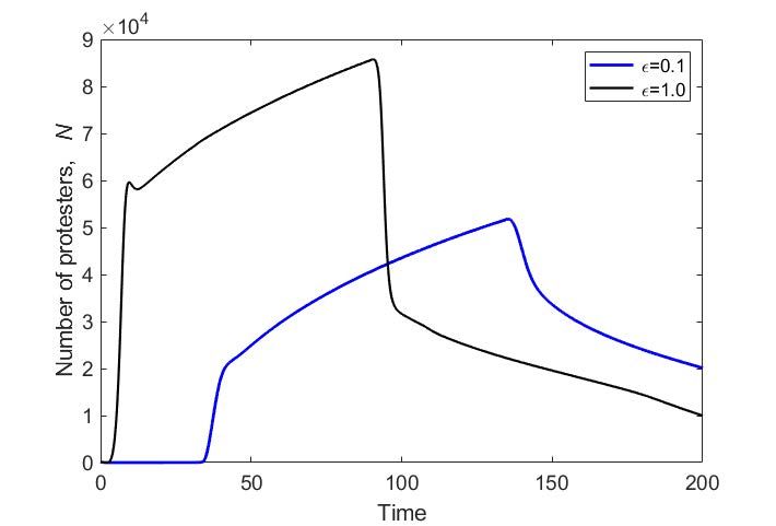
Mathematics 2020, 8, 78                                                                                     7 of 19

                                                      4

                                 Withdrawal rate, m
                                                      3

                                                          1

                                                      2

                                                      1
                                                                              2

                                                      0       50   100            150        200   250
                                                                   Number of protesters, N

      Figure 3. Phase plane of the system (7). The blue Curve 1 shows the N-isocline; note its part that lies
      close to the vertical axis. The red Curve 2 shows the solution of the system (obtained for parameters
      e0 = 0.1, e = 1, a = 115, h = 20, and β = 0.00025) where red arrows indicate the direction of the
      system’s evolution along the trajectory. The black arrows show the generic direction of the phase flow
      in different parts of the plane.

     In order to reveal the solution properties, the Equations (7) are solved numerically. We consider
β as the controlling parameter. Typical results are shown in Figure 4. At the beginning, the number
of protesters promptly becomes very large, thus creating a high peak (see Figure 4a). Past the peak,
the number of protesters starts falling, first fast, then at a decreasing rate. The number of protesters
keeps decreasing with time at a lower and lower rate until, at a certain moment, it promptly decays to
zero. The corresponding dependence m(t) is shown in Figure 4b.

                                                                         (a)

                                                                         (b)

      Figure 4. Solutions of Model (7) obtained for different values of β: (a) the number of protesters N vs.
      time and (b) the per capita withdrawal rate m vs. time. Other parameters are e0 = 0.1, e = 3, a = 115,
      and h = 20.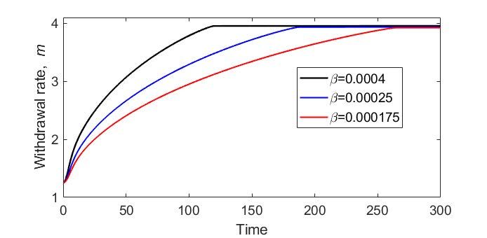
Mathematics 2020, 8, 78                                                                                8 of 19

     The behaviour of the solution of Model (7) is thus apparently similar to that of the solution of
the single component Model (1) and (2); cf. Figure 2. There are, however, some important differences.
In Model (1) and (2), there exists a finite critical value m∗ , so that for m0 < m∗ , the number of protesters
never falls to the small equilibrium value, but stabilizes at the higher steady state (see Curve 1 in
Figure 2a). On the contrary, in Model (7), there is no finite critical value: for any β > 0, the solution
N (t) will eventually converge to the lower steady state. We also note here that the shape of the graph
of N (t) shown in Figure 4a, albeit similar to Figure 2, is not the effect of the ghost attractor, but a
property of the so-called slow fast dynamics (when β  1) [31].

3. Spatially Explicit Model
      In the previous section, we completely disregarded the existence of the spatial dimension in the
dynamics of the social protests, hence implicitly assuming that the population density of the protesters
is distributed uniformly over space. In reality, it is rarely so, especially when the dynamics is considered
over a sufficiently large spatial scale such as a region, a county, a province, or the whole state. There
are several reasons for the spatial heterogeneity to emerge. Firstly, the overall population density itself
is distributed highly non-uniformly, i.e., reaching very high values in urban areas, but falling to low
values in the countryside. Secondly, people’s behavioural response and their social activity can be
significantly different at different locations in space, e.g., as a result of different living conditions and
different accessibility to social media. Therefore, although the consideration of non-spatial models
makes the first necessary step in the study, a more adequate mathematical framework for modelling
social protests must take space into account explicitly, as has indeed been recognized in a number of
studies, e.g., see [8,12–14]. In this section, we consider the models of the social protests dynamics in
space and time that consist of reaction-diffusion equations, where the “reaction” part is given by the
corresponding non-spatial model (as in Section 2) and the spread of the protests in space (described by
the diffusion terms) is regarded as a certain “contagion” [13,32].
      We mention here that the spatial spread of information and emotions and hence the spread of social
tensions are known to have two different spatial modes [12,32]. In one mode, people communicate in
direct encounters due to their geographical proximity: arguably, people living and/or working in the
same area would normally meet in person more frequently than people living far apart. The importance
of this mode of contagion is indirectly confirmed by the well established fact that most of everyday
human travel occurs within a short range from peoples’ homes [33]. In the second mode, the spread of
information and emotions is not related to travel and occurs due to the connection by social media.
For the first mode, the spread of protests can be described by the standard diffusion [12,14]; for the
second mode, kernel based integro-differential equations are thought to be more adequate [13] as they
better describe the effect of long distance connections [34]; see also [35–37].
      Note that, whilst the effect of the first mode is obviously limited to short distances, the second
mode is not restricted to any particular spatial scale: indeed, technically, social media can be accessed
from anywhere in the world. Hence, one can think, respectively, about the local coupling vs. the global
coupling. In the case of the local coupling due to direct encounters, the effect of space is likely to
be more pronounced; in particular, the level of social tensions should be a function of space. On the
contrary, in the case of the global coupling due to social media, the social tension is likely to be
distributed over space more uniformly.

3.1. Single Species Model
     We begin with the single species system. In terms of the above discussion, it corresponds to
the global coupling where the social tension is distributed over space uniformly, and hence, the
withdrawal rate does not depend on space (but depends on time). The distribution of the “population”
of protesters over space is then described by a single dynamical variable, i.e., by the population density,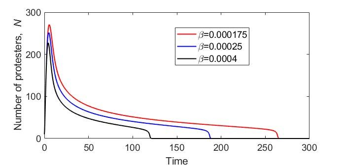
Mathematics 2020, 8, 78                                                                                 9 of 19

say u( x, t). The spatially explicit counterpart of Model (1) and (2) is described, in the 1D case, by the
following equation:
                                                      au2                  ∂2 u

                            ∂u( x, t)
                                      = e0 + eu + 2       2
                                                              − m(t)u + D 2 ,                           (8)
                               ∂t                   h +u                   ∂x
where x is the position in space, − L ≤ x ≤ L, D is the diffusion coefficient, and the dependence of the
withdrawal rate m on time is given by Equation (5).
    We assume that protests start at a certain location or a small area. Correspondingly, for the initial
conditions, we consider a piece-wise constant distribution of finite support described as follows:

                          u( x, 0) = u0 for − ∆ ≤ x ≤ ∆,           u( x, 0) = 0   otherwise.                (9)

      At the ends of the domain, we use the Dirichlet boundary condition, u(− L, t) = u( L, t) = 0.
      Equation (8) with (9) was solved numerically by finite differences. Typical results are shown in
Figure 5. We readily observe that the system dynamics are characteristic for reaction-diffusion systems
with compact initial conditions, albeit being modified by the dependence of the withdrawal rate on
time. At an early stage of the dynamics, the evolution of the initial distribution results in the formation
of two travelling fronts propagating away from the location of the initial condition (see the yellow,
violet, green, and light-blue curves in Figure 5a): the protests spread fast over space. In the course of
time, the speed of the fronts decreases as a result of the increase in m. Eventually, the front stops and
reverses (cf. the dark-blue and brown curves in Figure 5a). The population then retreats to the place
of its original introduction, which finally results in its collapse and extinction, i.e., the termination of
the protests.
                                Population density, u

                                                           space

                                                        (a)
                                Population density, u

                                                           space
                                                        (b)

      Figure 5. Solution of Model (8) shown at different moments of time (as is explained in the figure
      legend) obtained for m1 = 3 and different values of the final withdrawal rate: (a) for m0 = 5.4 and
      (b) for m0 = 5.8. Other parameters are e = 3, e1 = 0, a = 150, h = 35, b = 0.01, and D = 1.
Mathematics 2020, 8, 78 10 of 19
We mention here that we are not aware of any well developed mathematical theory of travelling
waves in non-autonomous reaction-diffusion systems, i.e., with reaction rates explicitly depending on
time. It seems, however, possible to explain the numerical results in terms of autonomous systems.
In the baseline case of constant m, the reaction term of Equation (8), that is:
au2
F (u) = e0 + eu + − mu, (10)
h2 + u2
is a sigmoidal curve, which, in the general case m∗ < m < m∗ (cf. Figure 1), has three roots,
0 ≤ ulower < uint < uhigher (where ulower = 0 if e0 = 0). The direction of the front propagation is
known to depend on the value of the following integral [38,39]:
Z u
higher
M= F (u)du, (11)
ulower
so that the front propagates towards the low density area (and hence away from the place of the
compact initial condition) if M > 0 and towards the high density area if M < 0. In the former case, the
protests invade, and in the latter case, the protests retreat.
In our case, m depends on time, and strictly speaking, the above results are not applicable.
However, one can expect that they may still work approximately. Indeed, it is readily seen that, for the
parameters chosen as in Figure 5, M > 0 at an early time, but becomes negative at a large time,
changing its sign at t ≈ 123 (see Figure 6). This explains the reversing of the front.
(a) (b)
Figure 6. Dependence on time of (a) M and (b) the speed of the front calculated in the course of the
travelling front propagation. The parameters are the same as in Figure 5a. It is readily seen that the
moment (t ≈ 123) when the front changes the direction of its propagation (invasion changes to retreat)
coincides with the moment when M changes its sign.
We therefore conclude that the spatial dynamics exhibits some new properties that did not exist
in its non-spatial counterpart, in particular by providing a new scenario of the termination of the
social unrest. Recall that, in the non-spatial system, the unrest terminates only after the increase in m
results in the disappearance of the upper positive steady state (see Figure 1). In the spatial system,
the unrest termination can happen even when the positive steady state exists: for the termination to
occur, it is sufficient that m becomes sufficiently large (but not necessarily supercritical) to reverse the
front propagation.
R
The dependence of the total number of protesters on time, i.e., Ntot (t) = [− L,L] u( x, t)dx, appears
to be rather different in the spatial system compared to the corresponding non-spatial system;
see Figure 7. Instead of the sharp peak, after the fast increase at the beginning, N (t) then exhibits a
much slower decrease than in the non-spatial system (cf. Figure 2), eventually accelerating to a fast
decay to zero.Mathematics 2020, 8, 78 11 of 19
Figure 7. Total number of protesters vs. time as given by the solution of Model (8) obtained for m0 = 5.4
(blue curve) and m0 = 5.8 (black curve). Other parameters are the same as in Figure 5.
3.2. Two Component Model
We now consider the spatially explicit version of Model (7), which is given by the following
equations:
∂u( x, t) au2 ∂2 u
= e0 + ( e − m ) u + +D 2, (12)
∂t h2 +u 2 ∂x
∂m( x, t) ∂2 m
= βu + Dm . (13)
∂t ∂x2
For the sake of generality, we assume that the spatial dynamics of the withdrawal rate may occur with
a different diffusion coefficient Dm .
For the initial conditions, similarly to the above, we consider the piece-wise constant distributions:
u( x, 0) = u0 for − ∆ ≤ x ≤ ∆, otherwise u( x, 0) = 0, (14)
m( x, 0) = m0 for − ∆m ≤ x ≤ ∆m , otherwise m( x, 0) = 0, (15)
where ∆m ≤ ∆ to reflect the assumption that there is no damage without protests. At the ends of the
domain, we use the Dirichlet boundary condition, u(− L, t) = u( L, t) = 0 and m(− L, t) = m( L, t) = 0.
Mathematical Problem (12)–(15) was solved numerically by finite differences using the forward
scheme. The mesh steps were chosen sufficiently small to avoid numerical artefacts, and it was checked
that a further decrease of the steps value had no effect on the numerical solution.
Some typical results are shown in Figure 8. We readily observe that, as well as in the previous
case, the evolution of the initial conditions results in the formation of two travelling waves propagating
away from the location of the initial distribution. However, the properties of the wave are essentially
different from those in the single species model. Instead of a smooth, monotonous front, we now
have a travelling peak with a very high population density at its maximum. In the wake of the
peak, the population density promptly decays to a much smaller value. The corresponding spatial
distribution of the withdrawal rate is shown in Figure 9. After the peak reaches the domain boundary,
it promptly disappears, and the total number of the protesters decays to zero.Mathematics 2020, 8, 78 12 of 19
Figure 8. Population density vs. space obtained as a solution of Model (12) and (13) shown at different
moments of time. Parameters are e0 = 0, e = 1, a = 115, h = 20, β = 0.00025, D = 1, and Dm = 0.1.
Figure 9. Distribution of the withdrawal rate over space as given by Model (12) and (13) shown at
different moments of time. Parameters are the same as in Figure 8.
As we observed in numerous numerical simulations, the main properties of the solution, such as
the formation of the population peaks propagating away from the location of the initial distribution,
were generic and robust to parameter changes. In particular, we did not observe any significant
changes in the system dynamics for different values of the diffusivity ratio Dm /D (having checked
several values of the ratio in the range between one and 0.01). However, some quantitative features of
the dynamics appeared to be somewhat sensitive to other parameter values. For instance, the height of
the peak depended on e rather strongly. An example shown in Figure 10 is obtained for e = 0.1. We
readily observe that, whilst the dynamics is qualitatively the same as in the case e = 1 (see Figure 8),
the height of the peak is almost an order of magnitude smaller. The speed of the peak propagation
is slightly less as well. The distribution of damage, however, shows features similar to what was
obtained for e = 1 (see Figure 9); we do not show it here for the sake of brevity.
R
Figure 11 shows the total number of protesters vs. time as is given by Ntot (t) = [− L,L] u( x, t)dx.
It is readily seen that the dynamics of the protests in the spatially explicit Model (12) and (13) is
considerably different from its non-spatial counterpart (7). Recall that in the non-spatial system, the
number of protesters reaches its maximum at early time and then decays monotonously, first very
fast and later at a decreasing rate (see Figure 4a). In the spatial system, however, the fast increase at
the beginning changes to a slower growth that goes on for a considerable length of time. The phase
of slow growth corresponds to the peak travelling over space where the shape of the peak remains
approximately the same, but the length of its tail grows steadily. The duration of this phase depends
on the extent of the available space; the larger the spatial domain is, the longer the total number ofMathematics 2020, 8, 78 13 of 19
protesters keeps growing slowly, but steadily. After the peak hits the boundary of the domain, the effect
of the boundary conditions bring it down, resulting in the sharp decrease in the protesters’ number.
Figure 10. Population density vs. space obtained as a solution of Model (12) for e = 0.1 shown at
different moments of time. Other parameters the same as in Figure 8.
Figure 11. Total number of protesters vs. time as given by the solution of Model (12) and (13) with
the initial conditions (14) and (15) obtained for e = 1 (black curve) and e = 0.1 (blue curve). Other
parameters are the same as in Figure 8.
Note that the collapse of the travelling wave as a result of the collision with the boundary is a
common phenomenon in reaction-diffusion systems of various origins [39–41]. Such a collapse is not
very sensitive to the type of the boundary condition; in particular, in our model, it was observed both
for the Dirichlet and Neumann types (for the sake of brevity, we do not show here the corresponding
figures for the zero-flux boundary conditions). We also mention that the collapse of protests observed
in our model when the wave reached the domain boundary could be insightful for understanding
the dynamics of real events of social unrest. For example, in the 2005 French riots, it was reported
that the street protests were quickly spreading across suburbs before they reached some quieter areas,
after which the whole unrest went extinct [13]. Although the collapse of the 2005 unrest in Paris can
be explained by a number of reasons, e.g., overall decrease of the protesters’ motivation, increasing
efficiency of the police, etc., reaching the edge of the area where the social or geographical conditions
changes significantly is arguably a major factor.
Apparently, the rate of increase in the total number of protesters depends on the speed of the
travelling peak. That raises an interesting mathematical question as to whether the speed can be
estimated. We recall here that, in reaction-diffusion systems, the travelling wave usually arises as aMathematics 2020, 8, 78 14 of 19
heteroclinic connection between two equilibria (homoclinic in the case of a travelling peak) in the
phase space of the system, the speed of the travelling wave being an eigenvalue of the corresponding
nonlinear problem [39,42,43]. Our system (12) and (13) does not quite fit into this framework, as a
positive equilibrium does not exist for e0 = 0. This indicates that, in a strict mathematical sense,
the travelling wave does not exist. However, arguably, the part of the solution that describes the
peak still behaves as a travelling wave, as indeed is readily seen from the properties of the numerical
solution, e.g., see Figures 8 and 10. Hence, we hypothesize that some of the tools normally used to
estimate the speed of the wave may still be applicable.
Such tools must be applied with due care though. We first observe that the solution behaves as a
travelling wave at the “leading edge” of the travelling peak, i.e., where both components u and m are
very small. Equation (12) can therefore be linearized taking the following very simple form:
∂u( x, t) ∂2 u
= eu + D 2 , (16)
∂t ∂x
where we consider e0 = 0 here and below for the sake of simplicity. Note that the linearized equation
does not contain m any more. For the linear reaction-diffusion equation with finite or semi-finite
initial condition, it is well known that, although the travelling wave solution does not exist globally,
the leading edge of the solution propagates as a travelling wave with the speed given by:
√
c = 2 eD, (17)
e.g., see [37,38]. Estimate (17) obtained by linearizing the system (12) and (13) therefore coincides with
the speed of the travelling front in a scalar reaction-diffusion equation with the generalized logistic
growth [42,43].
However, the expression (17) appears to be in bad disagreement with numerical results predicting
a value considerably less than was obtained in the simulations, e.g., two instead of 3.1 for the
parameters of Figure 8. Even worse, it does not in any way predict the dependence of the speed
on parameter values: for instance, for e = 0.1 Expression (17) gives c ≈ 0.63, whilst the actual value
is about 2.6. A more careful look readily reveals the reason for this disagreement: as a matter of fact,
Expression (17) is hardly relevant at all as its validity is limited to the case where the growth function
is convex [42,43], whilst in our case, it is not (see Figure 12).
We therefore have to apply a different approach, namely the approach based on the comparison
principle for PDEs [44]. We first notice that Equation (12) can be written as the following differential
inequality:
∂u( x, t) au2 ∂2 u
≤ eu + + D . (18)
∂t h2 + u2 ∂x2
We now build an auxiliary function F̃ (u) as follows:
F̃ (u) = αu for 0 ≤ u ≤ u A , (19)
au2
F̃ (u) = eu + 2 for u > u A , (20)
h + u2
where α is the slope of the tangent line to the graph of the reaction term and u A is the abscissa of the
conjunction point (Figure 12). After some simple algebra, we obtain that:
a
α= + e. (21)
2h
Obviously, F̃ (u) is an upper bound for the reaction term in the right hand side of (18), so that the
following inequality holds:Mathematics 2020, 8, 78 15 of 19
∂u( x, t) ∂2 u
≤ F̃ (u) + D . (22)
∂t ∂x2
By the virtue of the comparison principle, the solution of the following equation:
∂ũ( x, t) ∂2 ũ
= F̃ (ũ) + D . (23)
∂t ∂x2
gives an upper bound for the solution u( x, t) of Equation (12) provided the initial and boundary
conditions are the same.
Function F̃ (u) is convex; therefore, the linearization at the leading edge can be applied resulting,
taking (21) into account, in the following upper bound for the speed of the wave:
√
r
a
c = 2 αD = 2 + e D. (24)
2h
Growth rate
o
A
0
0
Population density
Figure 12. A sketch illustrating the idea of building an upper bound for the reaction term. The solid
(black) curve shows the reaction term in the right hand side of (18) (or Equation (12) with m ≡ 0), and
the dashed (blue) line shows the tangent line; see more details in the text.
Figure 13 shows the values of the speed calculated in simulations along with the analytical
estimate (24). It is readily seen that, while the expression (24) somewhat overestimates the actual
value, it manages to describes reasonably well the dependence of the speed on the parameter, i.e.,
the approximately linear increase along with an increase in e.
5
4
3
Speed
2
1
0
0.2 0.4 0.6 0.8 1 1.2 1.4
ε
Figure 13. Dependence of the speed of the travelling peak on e; diamonds show the numerical results,
and the blue line shows the analytical estimate (24).Mathematics 2020, 8, 78 16 of 19
4. Discussion and Concluding Remarks
Social protests are a complex phenomenon that has a variety of important implications for the
functioning of different social groups and organizations, as well as the society as a whole. Hence, a good
understanding of the protests’ dynamics is needed, in particular to identify the factors controlling their
intensity and duration and to reveal the generic patterns of the protests’ evolution in time and space.
Whilst this is apparently a problem in the remit of social sciences, mathematical modelling has long
been regarded as a powerful research tool that helps to achieve these goals [3,18].
In this paper, we considered a few generic, conceptual models of the social protests dynamics. We
disregarded the social structure of the crowd and described the dynamics by a single dynamic variable,
i.e., the number of protesters. Our study was partially motivated by the observation that there can be
two apparently different scenarios of the protests’ development in time: the one where the peak in the
total number of protesters is followed by a fast decay and the other one where the decay in the wake of
the main peak is very slow, thus creating a long tail. Correspondingly, our first goal was to understand
whether these two apparently different cases can be embraced in the framework of the same model. We
found that the two cases differed quantitatively rather than qualitatively, i.e., the different decay rate
(and hence, the total duration of the protests) was determined by the model parameters. Interestingly,
we obtained that the duration of the protests could, in principle, be indefinitely long, although the
corresponding parameter range was small.
There have been several studies previously where riots and social unrest were treated in terms of
nonlinear dynamical systems [2,11–13,17]. Adopting this modelling paradigm, the slow decay in the
protests intensity could be linked to the so-called long transient dynamics (cf. [17]): a phenomenon
inherent in many dynamical systems of different origin [30,31,45,46]. In a nutshell, a long transient
means that the dynamical system mimics its stable asymptotical dynamics (e.g., steady state, periodical,
or chaotic), being in fact in a transient regime. The quasi-asymptotical dynamics can persist for an
indefinitely long time before the system experiences a fast transition to its true asymptotics. In a
non-spatial system, the main mechanisms resulting in long transient are ghost attractors, crawl-bys,
and slow-fast dynamics [30,31], and this is precisely what determines that long tail predicted by our
models. The long tail obtained in the single species model (cf. Curves 1–3 in Figure 2b) was the effect
of the ghost attractor that emerged after the upper stable steady state of the system disappeared in a
saddle-node bifurcation when the final value of the withdrawal rate exceeded the critical value m∗ (see
Figure 1b). The long tail predicted by the two component model (e.g., see the green curve in Figure 4a)
was a manifestation of the slow-fast dynamics that arose for small values of β.
We mention here that linking our findings to some general properties of the dynamical systems
(such as the existence of long transient dynamics) is not a futile mathematical exercise, but brings
insights that can have immediate practical value. In particular, the generic property of long transients
that the slow decay in the protesters number is followed by a fast decay to zero may be used as a basis
for a response strategy: if the authorities have enough patience to wait (or other reasons not to use
excessive force in response to protests), it is likely that the protests eventually disappear due to their
inherent dynamics (perhaps this is what is happening with the 2019 riots in Hong Kong where the
authorities have been surprisingly mild in their response, probably just waiting until the riots burn out
by themselves).
The second goal of this study was to highlight the role of the spatial dimension in the dynamics of
social protests. We used mathematical modelling to reveal essential differences between the properties
of the spatial systems and their non-spatial counterparts. The importance of space is well recognized
in natural systems, in particular in ecology [22], but its effect on the social processes remains somewhat
obscure. We obtained that both models predicted the emergence of a travelling wave of the protests’
activity (albeit with rather different properties). This was in agreement with other recent modelling
studies [13,14]; also, the spatial dynamics reminiscent of a spreading wave was observed in some
data [13,47].Mathematics 2020, 8, 78 17 of 19
Our results suggested two essentially different scenarios of the protests’ development in space,
say, Type I and Type II. In the Type I scenario, the protesters are distributed over a certain area with
approximately uniform density, this area initially growing with time. The growth of the area “invaded”
by the protests is combined with a slow decrease in time (apart from a very early stage of the dynamics)
of the protesters’ population density uniformly over the whole invaded space, eventually resulting in
the protests shrinking back to the place of their origin and collapsing (see Figure 5). This is a result
of the global coupling where the withdrawal rate is the same everywhere in space: m depends on
time, but not on space. In the Type II scenario, the distribution of protesters over space is highly
heterogeneous. The large density of protesters is only observed inside a narrow range or small area,
which in the course of time moves away from the place where the protests started (see Figure 8).
The collapse of the protests occurs as a result of a specific “boundary forcing”, i.e., when the peaks
are pushed close to the domain boundary. This is a result of the interplay between the local coupling
(where, generally speaking, the withdrawal rate is different at different locations) and the feedback
mechanism through which the withdrawal rate depends on the protesters’ density. One can further
speculate as to how the difference between the two scenarios (and between the models, respectively)
can be projected onto real life. Since the explicit dependence of the withdrawal rate on space may
indicate the heterogeneity in the peoples’ responses, one can suggest that the Type I scenario is more
likely to occur in a well connected (hence global coupling), socially uniform society, while the Type II
scenario is more likely to be seen in a poorly connected society with a broader range of social norms.
Note that both non-spatial models that we considered in Section 2 describe a very similar pattern
in time, i.e., the main peak was followed by a tail, the rate of decay at the tail depending on the model
parameters. Since different models were built to account for the effect of different factors, that evokes
the old problem of the relation between the pattern and the process: if two different models predict the
same pattern, how do we “let the right one in”, i.e., what are the processes that are actually important?
However, when the models are extended to include space, the dynamics become qualitatively different.
Therefore, here, we showed that taking into account the spatial dimension of the system could be one
possible way to solve this problem.
Our study leaves a few open questions. Firstly, in our models, we assumed that the “population”
of protesters consisted of essentially identical individuals. In reality, people are different in terms
of beliefs, responses, social status, etc. [15,18,27,48,49]. How the heterogeneity of the population can
modify our findings remains unclear. In particular, the recruitment of protesters can be facilitated
by activists, as was the case in the Russian revolutions in 1905–1907 and later in 1917 [1,19,20].
Currently, such activists are active Internet users and social engineers and may have even a stronger
influence. Secondly, with regard to the spatial extension of the models, we restricted our analysis to the
hypothetical 1D case. How the patterns of spread may change in the more realistic 2D system remains
to be seen. Heterogeneity of space can also be an important factor affecting the dynamics of protests, as
was shown in a number of works [9,12,13], and that may require a mathematical framework different
from the standard Fickian diffusion, e.g., networks. Consideration of these factors should become a
focus of future research.
Author Contributions: The authors contributed equally to this work. All authors have read and agreed to the
published version of the manuscript.
Funding: The publication has been prepared with the support of the “RUDN University Program 5-100” (to S.P.).
Conflicts of Interest: The authors declare no conflict of interest.
References
1. Andreev, A.; Borodkin, L.; Levandovskii, M. Using methods of non-linear dynamics in historical social
research: Application of chaos theory in the analysis of the worker’s movement in pre-revolutionary Russia.
Hist. Soc. Res./Historische Sozialforschung 1997, 22, 64–83.Mathematics 2020, 8, 78 18 of 19
2. Epstein, J.M. Nonlinear Dynamics, Mathematical Biology, and Social Science; Addison-Wesley: Reading, MA,
USA, 1997.
3. Epstein, J.M. Modeling civil violence: An agent-based computational approach. Proc. Natl. Acad. Sci. USA
2002, 99 (Suppl. 3), 7243–7250. [CrossRef] [PubMed]
4. Turchin, P. Historical Dynamics: Why States Rise and Fall; Princeton University Press: Princeton, NJ, USA, 2003.
5. Eguiluz, V.M.; Zimmermann, M.G.; Cela-Conde, C.J.; San Miguel, M. Cooperation and emergence of role
differentiation in the dynamics of social networks. arXiv 2006, arXiv:physics/0602053v1.
6. Brantingham, P.J.; Tita, G.E.; Short, M.B.; Reid, S.E. The ecology of gang territorial boundaries. Criminology
2012, 50, 851–885. [CrossRef]
7. Fonoberova, M.; Fonoberov, V.A.; Mezic, I.; Mezic, J.; Brantingham, P.J. Nonlinear dynamics of crime and
violence in urban settings. J. Artif. Soc. Soc. Simul. 2012, 15, 2. [CrossRef]
8. Smith, L.M.; Bertozzi, A.L.; Brantingham, P.J.; Tita, G.E.; Valasik, M. Adaptation of an ecological territorial
model to street gang spatial patterns in Los Angeles. Discret. Contin. Dyn. Syst. 2012, 32, 3223–3244.
[CrossRef]
9. Davies, T.P.; Fry, H.M.; Wilson, A.G.; Bishop, S.R. A mathematical model of the London riots and their
policing. Sci. Rep. 2013, 3, 1303. [CrossRef]
10. Turalska MWest, B.J.; Grigolini, P. Role of committed minorities in times of crisis. Sci. Rep. 2013, 3, 1371.
[CrossRef]
11. Khosaeva, Z.H. The mathematics model of protests. Comp. Res. Model. 2015, 7, 1331–1341. (In Russian)
[CrossRef]
12. Berestycki, H.; Nadal, J.-P.; Rodíguez, N. A model of riots dynamics: Shocks, diffusion and thresholds. Netw.
Heterog. Media 2015, 103, 443–475. [CrossRef]
13. Bonnasse-Gahot, L.; Berestycki, H.; Marie-Aude Depuiset, M.A. Epidemiological modelling of the 2005
French riots: A spreading wave and the role of contagion. Sci. Rep. 2018, 8, 107. [CrossRef] [PubMed]
14. Yang, C.; Rodriguez, N. A numerical perspective on traveling wave solutions in a system for rioting activity.
Appl. Math. Comput. 2020, 364, 124646. [CrossRef]
15. Gavrilets, S. Collective action problem in heterogeneous groups. Philos. Trans. R. Soc. Lond. B 2015, 370,
20150016. [CrossRef] [PubMed]
16. Lang, J.C.; De Sterck, H. The Arab Spring: A simple compartmental model for the dynamics of a revolution.
Math. Soc. Sci. 2014, 69, 12–21. [CrossRef]
17. Morozov, A.; Petrovskii, S.V.; Gavrilets, S. Dynamics of Social Protests: Case study of the Yellow Vest
Movement. SocArXiv 2019. [CrossRef]
18. Granovetter, M. Threshold models of collective behavior. Am. J. Sociol. 1978, 83, 1420–1443. [CrossRef]
19. Haynes, M.J. Patterns of conflict in the 1905 revolution. In The Russian Revolution of 1905: Change through
Struggle; Glatter, P., Ed.; Porcupine Press: London, UK, 2005; pp. 215–233.
20. Perrie, M. The Russian peasant movement of 1905–1907: Its social composition and revolutionary significance.
Past Present 1972, 57, 123–155. [CrossRef]
21. Gelbwestenbewegung. Wikipedia. Available online: https://de.wikipedia.org/wiki/Gelbwestenbewegung
(accessed on 1 October 2019). (In German)
22. Malchow, H.; Petrovskii, S.V.; Venturino, E. Spatiotemporal Patterns in Ecology and Epidemiology: Theory, Models,
Simulations; Chapman & Hall/CRC Press: Boca Raton, FL, USA, 2008.
23. Gnedenko, B.V.; Kolmogorov, A.N. Limit Distributions for Sums of Independent Random Variables;
Addison-Wesley Mathematics Series; Addison-Wesley: Cambridge, MA, USA, 1954.
24. Altbach, P.G.; Klemencic, M. Student activism remains a potent force worldwide. Int. High. Educ. 2014, 76,
2–3. [CrossRef]
25. Mohamed, E.; Gerber, H.R.; Aboulkacem, S. (Eds.) Education and the Arab Spring; Sense Publishers: Rotterdam,
The Netherlands; Boston, MA, USA; Taipei, Taiwan, 2016.
26. Biggs, M. Size matters: Quantifying protest by counting participants. Sociol. Methods Res. 2018, 47, 351–383.
[CrossRef]
27. Raafat, R.M.; Chater, N.; Frith, C. Herding in humans. Trends Cognit. Sci. 2009, 13, 420–428. [CrossRef]
28. Courchamp, F.; Berek, L.; Gascoigne, J. Allee Effects in Ecology and Conservation; Oxford University Press:
Oxford, UK, 2008.Mathematics 2020, 8, 78 19 of 19
29. Schussman, A.; Soule, S.A. Process and protest: Accounting for individual protest participation. Soc. Forces
2005, 84, 1083–1108. [CrossRef]
30. Hastings, A.; Abbott, K.C.; Cuddington, K.; Francis, T.; Gellner, G.; Lai, Y.C.; Morozov, A.; Petrovskii,
S.; Scranton, K.; Zeeman, M.L. Transient phenomena in ecology. Science 2018, 361, eaat6412. [CrossRef]
[PubMed]
31. Morozov, A.; Abbott, K.; Cuddington, K.; Francis, T.; Gellner, G.; Hastings, A.; Lai, Y.C.; Petrovskii, S.;
Scranton, K.; Zeeman, M.L. Long transients in ecology: Theory and applications. Phys. Life Rev. 2019,
in press. [CrossRef]
32. Braha, D. Global civil unrest: Contagion, self-organization, and prediction. PLoS ONE 2012, 7, e48596.
[CrossRef]
33. Brockmann, D.; Hufnagel, L.; Theo Geisel, T. The scaling laws of human travel. Nature 2006, 439, 462–465.
[CrossRef]
34. Kendall, D.G. Discussion of “Measles periodicity and community size” by M.S. Bartlett. J. R. Stat. Soc. Ser. A
1957, 120, 64–67.
35. Mendez, V.; Fedotov, S.; Horsthemke, W. Reaction-Transport Systems: Mesoscopic Foundations, Fronts, and Spatial
Instabilities; Springer: Berlin, Germany, 2010.
36. Mendez, V.; Campos, D.; Bartumeus, F. Stochastic Foundations in Movement Ecology: Anomalous Diffusion,
Front Propagation and Random Searches; Springer: Berlin, Germany, 2014.
37. Lewis, M.A.; Petrovskii, S.V.; Potts, J. The Mathematics behind Biological Invasions; Interdisciplinary Applied
Mathematics; Springer: Berlin, Germany, 2016; Volume 44.
38. Murray, J.D. Mathematical Biology; Springer: Berlin, Germany, 1989.
39. Volpert, A.; Volpert Vit Volpert, V.L. Traveling Wave Solutions of Parabolic Systems; AMS: Providence, RI,
USA, 1994.
40. Fife, P.C. Mathematical Aspects of Reacting and Diffusing Systems; Lecture Notes in Biomathematics; Springer:
Berlin, Germany, 1979; Volume 28.
41. Zeldovich, Y.B.; Barenblatt, G.I.; Librovich, V.B.; Makhviladze, G.M. The Mathematical Theory of Combustion
and Explosions; Consultants Bureau: New York, NY, USA, 1985.
42. Kolmogorov, A.N.; Petrovskii, I.G.; Piskunov, N.S. A study of the diffusion equation with increase in the
quantity of matter, and its application to a biological problem. Bull. Moscow Univ. Math. Ser. A 1937, 1, 1–25.
43. Kolmogorov, A.N.; Petrovskii, I.G.; Piskunov, N.S. A study of the diffusion equation with increase in the
amount of substance, and its application to a biological problem. In Selected Works of A. N. Kolmogorov;
Tikhomirov, V.M., Ed.; Kluwer Academic: Dordrecht, The Netherlands, 1991; pp. 242–270.
44. Protter, M.H.; Weinberger, H.F. Maximum Principles in Differential Equations; Springer: New York, NY,
USA, 1984.
45. Hastings, A.; Higgins, K. Persistence of transients in spatially structured ecological models. Science 1994, 263,
1133–1136. [CrossRef]
46. Lai, Y.C.; Tél, T. Transient Chaos—Complex Dynamics on Finite-Time Scales; Springer: New York, NY, USA, 2011.
47. Map of White Supremacy Mob Violence. Available online: http://www.monroeworktoday.org/explore/
(accessed on 1 October 2019).
48. Homer-Dixona, T.; Maynardb, J.L.; Mildenbergerc, M.; Milkoreita, M.; Mocka, S.J.; Quilleyd, S.; Schröder, T.;
Thagarde, P. A complex systems approach to the study of ideology: Cognitive-affective structures and the
dynamics of belief systems. J. Soc. Political Psychol. 2013, 1, 337–363.
49. Mistry, D.; Zhang, Q.; Perra, N.; Baronchelli, A. Committed activists and the reshaping of the status-quo
social consensus. Phys. Rev. E 2015, 92, 042805. [CrossRef]
c 2020 by the authors. Licensee MDPI, Basel, Switzerland. This article is an open access
article distributed under the terms and conditions of the Creative Commons Attribution
(CC BY) license (http://creativecommons.org/licenses/by/4.0/).You can also read