An adaptive space-time phase field formulation for dynamic fracture of brittle shells based on LR NURBS
←
→
Page content transcription
If your browser does not render page correctly, please read the page content below
An adaptive space-time phase field formulation for
                                                    dynamic fracture of brittle shells based on LR NURBS

                                                           Karsten Paul∗ , Christopher Zimmermann∗ , Kranthi K. Mandadapu†§ ,
                                                               Thomas J.R. Hughes‡ , Chad M. Landis‡ , Roger A. Sauer∗1

                                                     ∗
                                                         Aachen Institute for Advanced Study in Computational Engineering Science (AICES),
                                                               RWTH Aachen University, Templergraben 55, 52062 Aachen, Germany
                                                                       †
                                                                     Department of Chemical and Biomolecular Engineering,
                                                    University of California at Berkeley, 110A Gilman Hall, Berkeley, CA 94720-1460, USA
                                                      §
                                                          Chemical Sciences Division, Lawrence Berkeley National Laboratory, CA 94720, USA
                                                                  ‡
                                                                    The Oden Institute for Computational Engineering and Sciences,
arXiv:1906.10679v2 [cs.CE] 18 Jun 2020

                                                                  The University of Texas at Austin, 201 E. 24th Street, POB 4.102,
                                                                     1 University Station (C0200), Austin, TX 78712-1229, USA

                                                              Published2 in Comput. Mech., DOI: 10.1007/s00466-019-01807-y
                                                 Submitted on 28. June 2019, Revised on 20. September 2019, Accepted on 21. November 2019

                                         Abstract
                                         We present an adaptive space-time phase field formulation for dynamic fracture of brittle shells.
                                         Their deformation is characterized by the Kirchhoff-Love thin shell theory using a curvilinear
                                         surface description. All kinematical objects are defined on the shell’s mid-plane. The evolution
                                         equation for the phase field is determined by the minimization of an energy functional based
                                         on Griffith’s theory of brittle fracture. Membrane and bending contributions to the fracture
                                         process are modeled separately and a thickness integration is established for the latter. The
                                         coupled system consists of two nonlinear fourth-order PDEs and all quantities are defined on an
                                         evolving two-dimensional manifold. Since the weak form requires C 1 -continuity, isogeometric
                                         shape functions are used. The mesh is adaptively refined based on the phase field using Locally
                                         Refinable (LR) NURBS. Time is discretized based on a generalized-α method using adaptive
                                         time-stepping, and the discretized coupled system is solved with a monolithic Newton-Raphson
                                         scheme. The interaction between surface deformation and crack evolution is demonstrated by
                                         several numerical examples showing dynamic crack propagation and branching.
                                         Keywords: Phase fields, brittle fracture, isogeometric analysis, adaptive local refinement, LR
                                         NURBS, nonlinear finite elements, Kirchhoff-Love shells

                                         1        Introduction

                                         The need for shortening development cycles of engineering components requires efficient compu-
                                         tational methods. The robustness requirements for these components are increasing so that the
                                         prediction of structural defects and failure plays a major role in current development processes.
                                         It is therefore important to have efficient and reliable computational methods for predicting
                                             1
                                                 corresponding author, email: sauer@aices.rwth-aachen.de
                                             2
                                                 This pdf is the personal version of an article whose final publication is available at link.springer.com.

                                                                                                      1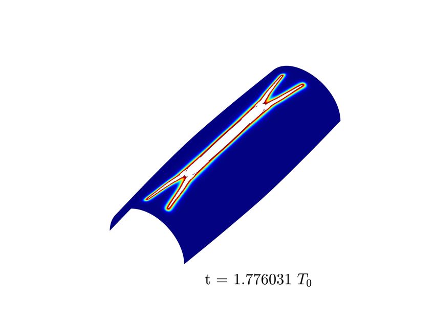
fracture. Several computational methods have been introduced to model crack growth. The
most important ones in the framework of finite elements are described subsequently.
Sharp interface models introduce discontinuities within the body in order to model cracks. In
the extended finite element method by Moës et al. (1999), the basis functions are enriched by
discontinuities to model the displacement jump across cracks. In contrast to this, a crack can be
introduced by a modification of the finite element mesh as in the virtual crack closure technique
(Krueger, 2004). Similar to the extended finite element method, Remmers et al. (2003) also enrich
the basis in the cohesive segments method. Several of these sharp interface models have been used
to model dynamic fracture and fragmentation. Ortiz and Pandolfi (1999) introduce cohesive
elements in a large deformation framework to track evolving cracks in a dynamic framework.
Fragmentation stemming from high loading rates is investigated by Molinari et al. (2007) within
the small strain regime, based on the cohesive element approach. In Papoulia (2017), a cohesive
model based on a non-differentiable energy functional is outlined. They add a momentum term
to the latter to enable the use of implicit time-stepping. The latter has been further advanced
by Vavasis et al. (2020). In Hirmand and Papoulia (2018), a discontinuous Galerkin-formulation
is used to model dynamic fracture. They employ Newmark’s time integration scheme and use
a trust region minimization approach to solve the smooth non-convex problems that occur in
their formulation. Geelen et al. (2018) combine a phase field formulation with an extended
finite element method by using a diffuse crack tip and a sharp traction-free crack behind it. In
Radovitzky et al. (2011), a combination of a discontinuous Galerkin-formulation and a cohesive
zone model is presented. This combination ensures stability and robustness prior to the onset
of fracture and shows good scalability with respect to computation time. Geelen et al. (2019)
consider cohesive fracture and investigate a novel degradation function and different approaches
to enforce an irreversible fracture process. Explicit and implicit time integration schemes are
compared in a dynamic cohesive fracture framework in Hirmand and Papoulia (2019). Their
formulation leads to a flexible framework that is easy to implement into existing standard finite
element frameworks. In general, the location of the crack has to be known in sharp interface
models. Thus, it has to be numerically tracked, which tends to be a complex task, especially in
three dimensions.
Thus, diffuse interface models have gained popularity for modeling brittle fracture. In the phase
field method no discontinuities are introduced within the body. Instead, the crack is smoothed
out and described by a small transition zone that ranges between undamaged and fully fractured
material. Phase field methods describe the evolving cracks by an additional partial differential
equation (PDE) such that there is no need for tracking the interface. For complex crack patterns
including nucleation, branching, and merging, phase field formulations have been shown to be
very effective.
Based on the thermodynamic considerations of brittle fracture by Griffith (1921), a variational
formulation of brittle fracture has been introduced by Francfort and Marigo (1998). Their
formulation includes the minimization of a global energy functional to model the quasi-static
fracture process. A corresponding phase field implementation within the finite element method
has been presented by Bourdin et al. (2000). The robustness and accuracy of the variational
formulation in two and three dimensions using phase field methods have been demonstrated by
e.g. Miehe et al. (2010a) and Miehe et al. (2010b). Successful extensions to dynamic problems
have been presented by Larsen et al. (2010), Larsen (2010), Bourdin et al. (2011), Borden et al.
(2012), Hofacker and Miehe (2013) and Schlüter et al. (2014). In contrast to the variational
formulation of brittle fracture, Karma et al. (2001) and Kuhn and Müller (2010) use a phase
transition framework based on the Ginzburg-Landau equation. The latter is more often used
in the physics community. Its derivation is based on general phase separation processes and
small adjustments are required for fracture, for instance to avoid crack healing. In these models,

                                                2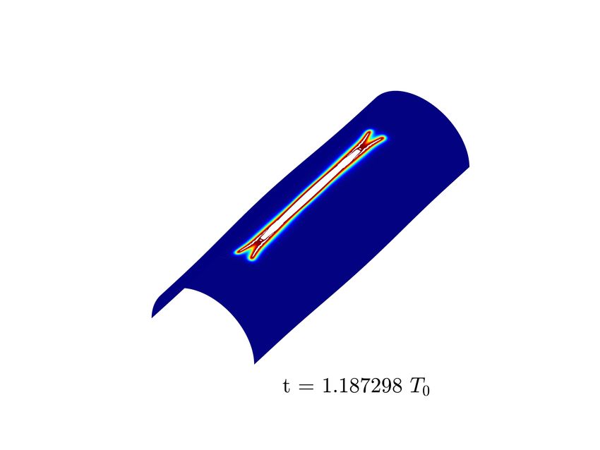
the onset of brittle fracture is not seen as instantaneous, but obeying its own gradient-based
dynamics. A stabilization for quasi-static simulations using a monolithic solution approach
for the coupled system is proposed by Gerasimov and Lorenzis (2016). Heister et al. (2015)
convexify their energy functional to obtain a positive definite Hessian matrix for monolithic
coupling. Gerasimov et al. (2018) apply a non-intrusive global/local approach in a phase field
framework for brittle fracture, in which at first the structural analysis of the whole domain
is performed and, afterwards, local regions where fracture is predicted are re-analyzed. These
steps are then repeated until convergence is obtained. Ambati et al. (2015) summarize several
phase field formulations for brittle fracture. In the work of Kuhn et al. (2015), the influence
of different degradation functions on the solution is investigated. Similar investigations are
made by Sargado et al. (2018) who also study parametric degradation functions. Possibilities
to enforce irreversibility of the fracture process are presented in detail in the work of Gerasimov
and Lorenzis (2019), especially focusing on the penalty method. The authors also derive a lower
bound for the penalty parameter for a quasi-static second-order phase field model for brittle
fracture.
The majority of the published phase field methods for fracture use a second-order phase field
formulation. The high order differential operators of the phase field PDE stemming from the
crack density functional of Borden et al. (2014), which is used in this work, and the equation
of motion of the shell framework require a spatial finite element discretization that is at least
C 1 -continuous. Isogeometric Analysis (IGA), proposed by Hughes et al. (2005), allows for
user-defined smoothness of the solution within the finite element framework. Within IGA,
the smoothness is most commonly achieved through the use of B-Spline- and NURBS-based
shape functions. Since phase field methods require a highly resolved finite element mesh in
the transition zone, local refinement methods are commonly used in the context of phase field
methods for fracture. The introduction of hierarchical B-splines by Forsey and Bartels (1988)
has offered the possibility of local refinement within an IGA framework. The extension to the
local refinement of NURBS is for instance given by Sederberg et al. (2003) by introducing T-
Splines. Another approach that allows local refinement is Locally Refinable (LR) splines. LR
B-splines were first introduced by Dokken et al. (2013) and further advanced by Johannessen
et al. (2014). Their extension to LR NURBS is provided by Zimmermann and Sauer (2017).
A combination of LR and T-splines is given by Chen and de Borst (2018) by the introduction
of LR T-splines. In constrast to LR splines, LR T-splines take a T-mesh as input instead of a
tensor-product mesh. Isogeometric collocation methods (Gomez et al., 2014; Reali and Hughes,
2015) for phase field models of fracture are also introduced, for instance by Schillinger et al.
(2015).
Hesch et al. (2016b) employ a hierarchical refinement scheme within a higher order phase field
model. Similarly, Hesch et al. (2016a) couple a model for frictional contact to a higher order
phase field model using hierarchical NURBS. Kästner et al. (2016) investigate phase field models
by comparing adaptive refinement based on locally refined hierarchical B-splines with uniformly
refined discretizations. Borden et al. (2012) propose an adaptive refinement strategy using T-
splines and use the phase field value itself to identify the need for local refinement. Mesh
adaptivity schemes, in which a predictor-corrector scheme is used, are employed by Zhou and
Zhuang (2018) for modeling fracture in rocks and by Badnava et al. (2018) to model mechanically
and thermo-mechanically induced cracks. In these approaches, the system is solved and then
checked for the need of mesh refinement. A similar approach is employed by Heister et al. (2015).
In the work by Nagaraja et al. (2018), a multi-level hp-refinement technique is established using
the finite cell method (Parvizian et al., 2007) to model brittle fracture in two dimensions. Chen
et al. (2018) employ LR T-splines for discrete fracture analysis. They insert mesh lines to obtain
discontinuous basis functions that are able to represent sharp cracks.

                                                3
Many papers concerning the computational modeling of shells within an isogeometric framework
have been published, for instance by Benson et al. (2013), Echter et al. (2013), Kiendl et al.
(2015) and Duong et al. (2017). Since for shells the bending stress varies across the thickness,
a suitable split of the energy within the fracture model has to be established. In the work by
Ulmer et al. (2012), brittle fracture in thin plates and shells is modeled. They combine a plate
and a standard membrane to model the shell but only split the membrane and not the bending
part of the elastic energy. Thus, the whole bending energy contributes to crack evolution and is
degraded in regions of damage. Amiri et al. (2014) do not employ an energy split, which limits
their model to shells under pure tension. In the work by Ambati and De Lorenzis (2016), the
shell and the phase field are also discretized over the thickness. Areias et al. (2016) utilize two
phase fields, one for the top and the other one for the bottom face of the shell. This framework
is also used by Reinoso et al. (2017) for a 6-parameter shell model. Their formulation results
in a non-constant phase field throughout the thickness. In contrast to this, Kiendl et al. (2016)
use a constant phase field over the thickness but use thickness integration to split the whole
energy into a tensile part, which contributes to crack growth, and a compressive part, which
does not.
Zimmermann et al. (2019) model Cahn-Hillard phase field equations on deforming surfaces
based on the shell formulation of Duong et al. (2017). Even though a different physical process
is modeled, the resulting coupled finite element formulation is similar to the one proposed here.
In this paper we establish a dynamic brittle fracture framework within the nonlinear IGA thin
shell formulation of Duong et al. (2017), in which shells with arbitrarily large curvature or doubly
curved shells can be modeled. Its hyperelastic material model allows for large deformations and
is given as a sum of membrane and bending contributions. The proposed higher order phase
field model of Borden et al. (2014) is adopted because of its higher rate of convergence and it
is formulated on the shell’s mid-plane. Motivated by the work of Kiendl et al. (2016), bending
effects on the fracture process are modeled based on thickness integration. Adaptive spatial
refinement is based on LR NURBS (Zimmermann and Sauer, 2017) and temporal discretization
is based on the generalized-α scheme (Chung and Hulbert, 1993). The time steps are adjusted
based on the number of Newton-Raphson iterations required during the last time step. In
summary, the proposed formulation contains the following features:

   • It couples a higher-order phase field model for fracture with a nonlinear shell formulation.

   • It is formulated in curvilinear coordinates, and applicable to general shell configurations.

   • The coupled system is solved within a monolithic, fully implicit solution approach.

   • It uses adaptive local refinement in space and time.

   • The spatial discretization is based on LR NURBS.

   • An energy split is used in which the membrane and bending energies are split separately.

The subsequent sections are structured as follows: Sec. 2 summarizes the surface description
and kinematics. The balance laws and the equation of motion are derived in Sec. 3. Sec. 4
introduces the energy minimization problem and the material model employed. Extensions to
degradation, irreversibility and an energy split are also presented. Based on the Euler-Lagrange
equation, the Helmholtz free energy is minimized, which leads to the governing equation for
the phase field’s evolution. The discretization of the coupled problem is described in Sec. 5.
Numerical examples are presented in Sec. 6 to illustrate crack propagation on curved surfaces.
Conclusions are drawn in Sec. 7.

                                                 4
2     Deforming surfaces

This section summarizes the thin shell formulation in the framework of curvilinear coordinates
and Kichhoff-Love kinematics. A more detailed presentation can be found in Sauer (2018).

2.1   Surface description

A curved surface S in 3D space can be characterized by the parametric description at any time
t by the function
                                  x = x(ξ α , t) , α = 1, 2 ,                              (1)
where ξ α denote the curvilinear coordinates associated with a material point x ∈ S. ξ α are
convected along with the material deformation of the surface and hence, they are also called
convected coordinates. The co-variant tangent vectors at x are given by
                                                      ∂x
                                           aα :=           .                                   (2)
                                                      ∂ξ α
From these follow the surface metric

                                         aαβ := aα · aβ ,                                      (3)

the surface normal
                                                 a1 × a2
                                         n :=              ,                                   (4)
                                                ka1 × a2 k
and the contra-variant tangent vectors

                                          aα = aαβ aβ ,                                        (5)

where [aαβ ] = [aαβ ]−1 . All Greek indices range from 1 to 2 and are summed when repeated.
Based on the second parametric derivative aα,β := ∂aα /∂ξ β , the curvature tensor components

                                         bαβ = aα,β · n ,                                      (6)

follow. The set of initial surface points X ∈ S0 follows from X := x(ξ α , 0). In analogy
to Eqs. (2)–(6), we define the surface quantities Aα := ∂X/∂ξ α , Aαβ := Aα · Aβ , N :=
A1 × A2 /kA1 × A2 k, Aα := Aαβ Aβ , [Aαβ ] := [Aαβ ]−1 and Bαβ := Aα,β · N at t = 0 as a
reference configuration, denoted S0 . The surface gradient

                                   gradS φ = ∇S φ := φ;α Aα ,                                  (7)

and surface Laplacian
                                 ∆S φ := ∇S · ∇S φ = φ;αβ Aαβ ,                                (8)
can be defined based on the parametrization in Eq. (1). Here, φ denotes a general scalar function
and the subscript ‘;’ indicates the co-variant derivative. It is equal to the parametric derivative
for general scalars, i.e. φ;α = φ,α := ∂φ/∂ξ α . But, φ;αβ 6= φ,αβ and instead

                                     φ;αβ = φ,αβ − Γ̂γαβ φ,γ ,                                 (9)

where Γ̂γαβ = Aα,β · Aγ are the Christoffel symbols of the second kind on surface S0 . On S,
these read Γγαβ = aα,β · aγ .

                                                  5
2.2   Surface kinematics

The relation between reference surface S0 and current surface S is described by the surface
deformation gradient
                                       F = aα ⊗ Aα .                                   (10)
The left surface Cauchy-Green tensor then follows as

                                          B = Aαβ aα ⊗ aβ ,                              (11)

with its two invariants
                                                           p
                          I1 := Aαβ aαβ       and J :=      det[Aαβ ] det[aαβ ] .        (12)

The latter characterizes the surface stretch between S0 and S. The surface Green-Lagrange
strain tensor and the symmetric relative curvature tensor are
                                      1
                                  E =   (aαβ − Aαβ ) Aα ⊗ Aβ ,
                                      2                                                  (13)
                                  K = (bαβ − Bαβ ) Aα ⊗ Aβ .

The material time derivative is denoted by

                                            ˙ := ∂...
                                          (...)                        .                 (14)
                                                 ∂t      ξ α = fixed

This leads to the material velocity at x

                                                v := ẋ ,                                (15)

and the rates
                                     ∂v
                      ȧα = v ,α =        ,    and ȧαβ = aα · ȧβ + ȧα · aβ .          (16)
                                     ∂ξ α

2.3   Surface variations

The variation of various surface measures is required for the formulation of the weak form of
the thin shell equation. Particularly important are the variations

                                  δaαβ = aα · δaβ + δaα · aβ ,
                                  δbαβ = δaα,β − Γγαβ δaγ · n ,

                                                                                         (17)
                                  δn      =   −(aα   ⊗ n) δaα ,

where δaα = δx,α and δaα,β = δx,αβ . Here, δx denotes a kinematically admissible variation of
the deformation. Additional variations of surface quantities are provided in Sauer and Duong
(2017).

3     Thin shell theory

The governing equations for the shell are summarized in the following. Equilibrium is given
in strong and weak form. Considering Kirchhoff-Love kinematics, the constitutive behavior of
thin shells can be fully characterized by the quantities aαβ and bαβ .

                                                     6
3.1     Balance of linear and angular momentum

The equation of motion
                                        ρ v̇ = T α;α + f ,      ∀x ∈ S ,                         (18)
follows from the balance of linear momentum for surface S. f = f α aα + p n denotes prescribed
body forces and
                                     T α = N αβ aβ + S α n ,                              (19)
are the stress vectors that include the in-plane membrane components N αβ and the out-of-
plane shear components S α (Naghdi, 1973; Steigmann, 1999; Sauer and Duong, 2017). These
are related to the stress tensor

                                    σ = N αβ aα ⊗ aβ + S α aα ⊗ n ,                              (20)

through Cauchy’s formula T α = σ T aα . Given the outward pointing normal ν = να aα at a cut
through S, the traction T = σ T ν = T α να acting on this cut follows.
Likewise, the moment vector on the cut reads M = µT ν with the moment tensor

                                           µ = −M αβ aα ⊗ aβ ,                                   (21)

where M αβ denotes its in-plane components (Sauer and Duong, 2017; Sahu et al., 2017). The
balance of angular momentum yields
                                                        βα
                                               S α = −M;β  ,
                                                                                                 (22)
                                               σ αβ = σ βα ,

where σ αβ := N αβ − bβγ M γα . The stress components σ αβ and M αβ follow from constitution,
which is discussed in Sec. 4.2.
The component form of the equation of motion
                                                      λα − S λ bα ,
                                       ρ aα = f α + N;λ         λ
                                                                                                 (23)
                                       ρ an = p + N αβ bαβ + S;α
                                                              α ,

is obtained by combining Eqs. (18), (20) and (22.1). Here, aα := v̇ · aα , an := v̇ · n, f α := f · aα
and p := f · n.

3.2     Weak form for deforming thin shells

The weak form for Kirchhoff-Love shells is given by (Sauer and Duong, 2017; Sauer et al., 2017)

                                Gkin + Gint − Gext = 0 ,           ∀ δx ∈ U ,                    (24)

with                           Z
                     Gkin :=        δx · ρ v̇ da ,
                                S
                               Z                Z
                                  1        αβ
                     Gint   :=      δaαβ σ da +    δbαβ M αβ da ,                                (25)
                                S 2              S
                               Z              Z             Z
                     Gext   :=    δx · f da +   δx · T ds +       δn · M ds .
                                S                    ∂t S              ∂m S
Here,                 n                                                   o
                   U = δx ∈ H̃2 S(x, t)3 | δx = 0 on ∂x S , δn = 0 on ∂n S ,

                                                                                                 (26)

                                                            7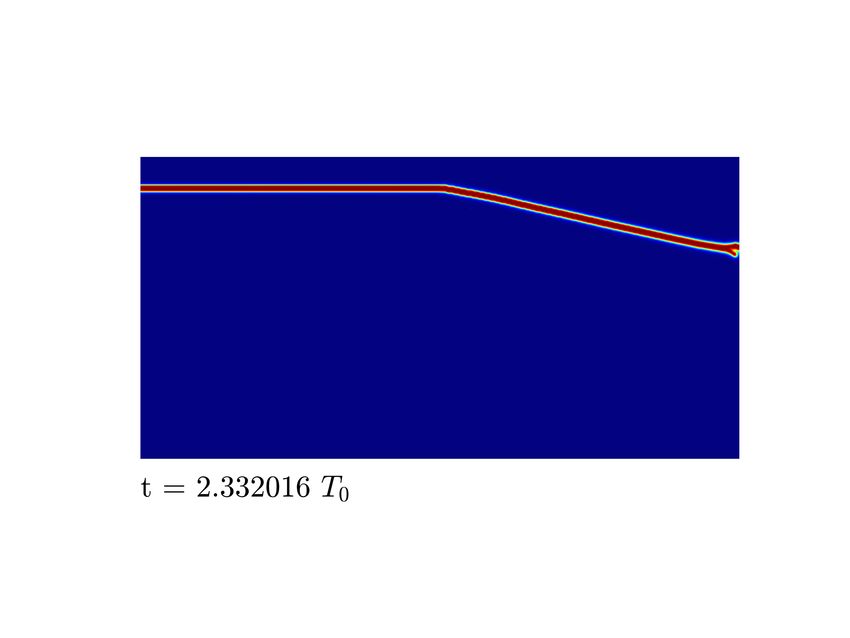
is the space of suitable surface variations, where H̃2 is the Sobolev space of Lebesgue square inte-
grable functions and ∂x S and ∂n S are the Dirichlet boundaries for displacements and rotations.
The prescribed edge tractions T = σ T ν and edge moments M = µT ν act on the boundaries
∂t S and ∂m S with the outward normal ν = να aα . We note that the torsional components of
the moment M are perceived as an effective shear traction in Kirchhoff-Love shells, e.g. see
Sauer and Duong (2017). If desired, da = J dA and ρ da = ρ0 dA can be used to map integrals
to the reference surface S0 . The components σ αβ and M αβ follow from the constitutive laws as
outlined in Sec. 4.2.

4     Fracture of deforming surfaces

The formulation for the modeling of brittle fracture is based on Griffith’s theory (Griffith, 1921),
in which the energy release rate EG of a body, which describes the dissipated energy during crack
evolution, is related to the fracture toughness Gc [J m−1 ]. The latter is also referred to as the
critical fracture energy density or critical energy release rate. The corresponding Kuhn-Tucker
conditions read
                          EG − Gc ≤ 0,        ċ ≥ 0,    (EG − Gc ) ċ = 0 ,                    (27)
with ċ denoting the crack propagation velocity. Since crack nucleation and branching are not
captured by this formulation, Griffith’s theory has been reformulated as a global energy mini-
mization problem (Francfort and Marigo, 1998). The corresponding energy functional is derived
subsequently.

4.1   Helmholtz free energy

The total energy in the system is given by
                                     Π := Πint + Πkin − Πext ,                                 (28)
where the three contributions denote the Helmholtz free energy Πint , the kinetic energy Πkin
and the external energy Πext , respectively. Based on the formulation of energy minimization
by Francfort and Marigo (1998), the Helmholtz free energy contains elastic and fracture energy
contributions in the form
                              Z           Z h                        i
                       Πint =    Ψ dA =       g(φ)Ψ+
                                                   el + Ψ −
                                                          el + Ψ frac dA ,                (29)
                                S0           S0

where Ψ denotes the Helmholtz free energy per reference area. Cracks resemble discontinuities
in the deformation that are smeared out in the phase field formulation. Therefore, an indicator
φ ∈ [0, 1] is established that distinguishes between fully fractured, φ = 0, and undamaged,
φ = 1, material. This field is referred to as the phase field or fracture field. Since it models the
damage region, it is used to define the fracture energy appearing in Eq. (29). The higher order
phase field model by Borden et al. (2014) is adopted here, which, expressed in variables of the
present thin shell formulation, reads
                                Gc h                                          i
                       Ψfrac =       (φ − 1)2 + 2`20 ∇S φ · ∇S φ + `40 (∆S φ)2 .                (30)
                                4`0
The length scale parameter `0 [m] controls the support width of the transition zone: supp(φ) ∼
`0 . Borden et al. (2014) have shown that the one-dimensional phase field approximation of the
crack surface Γ = {0} has the form

                                                 |x|       |x|
                               φ(x) = 1 − exp −        1+        ,                        (31)
                                                 `0        `0

                                                  8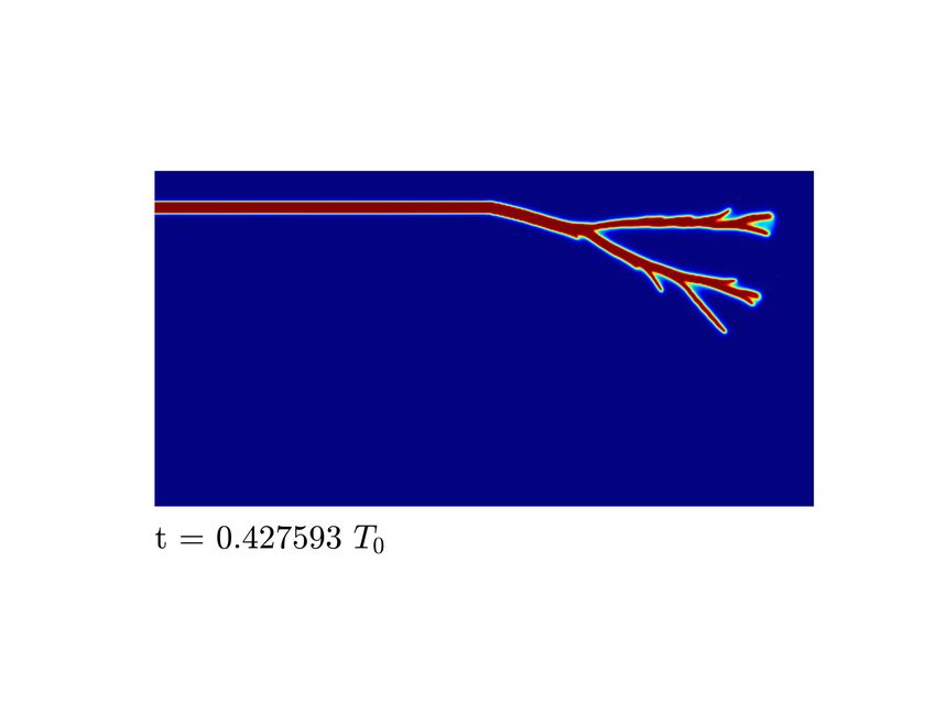
which is illustrated in Fig. 1.

                        1

                 φ(x)

                                                                  crack surface Γ
                                                                  φ(x)
                        0
                                                −2`0 0 2`0
                                                     x

Figure 1: Phase field profile for the fourth-order theory of Borden et al. (2014). The crack
surface Γ = {0} is smoothed by the function φ(x) from Eq. (31).

An additive energy split is required in which the elastic energy density is split into a part
that contributes to crack evolution (‘+’) and a part that has no effect on crack growth (‘−’):
Ψel = Ψ+       −
        el + Ψel . The two contributions are also referred to as the positive and negative part of
the elastic energy density. The split is further motivated and derived in Sec. 4.2.1. According
to Eq. (29), the positive part of the elastic energy density Ψ+el is degraded through g(φ) along
the damage regions. Here, it is assumed to take the form (Borden et al., 2016)
                                   g(φ) = (3 − s)φ2 − (2 − s)φ3 ,                            (32)
where s > 0 describes the slope of g(φ) at φ = 1. If s = 0, a surface without initial damage would
fulfill the governing equation for crack evolution in Eq. (60) for any deformation implying that
crack nucleation would not occur. Thus, s is set to 10−4 (Borden et al., 2016) in all subsequent
computations to allow crack nucleation in the absence of initial damage. Degradation functions
with g 0 (1) = 0 could be used but they require a perturbation in the first Newton-Raphson
iteration to allow for crack nucleation in sound materials (Kuhn et al., 2015).

4.2   Hyperelastic material model

The elastic energy density Ψel is taken as an additive composition of dilatational, deviatoric
and bending energy densities in the form
                            Ψel = Ψdil (aαβ ) + Ψdev (aαβ ) +Ψbend (bαβ ) ,
                                  |           {z         }                                   (33)
                                          Ψmem (aαβ )

where the first two terms describe the membrane part of Ψel . A Neo-Hookean surface material
model (Sauer and Duong, 2017) with
                                             K 2
                                    Ψdil =     J − 1 − 2 ln J ,                              (34)
                                             4
and
                                             G
                                       Ψdev =   I1 /J − 2 ,                               (35)
                                              2
is used to model the isotropic in-plane constitutive response. K refers to the 2D bulk modulus
and G to the 2D shear modulus. The bending response follows from the Koiter model (Ciarlet,
1993)
                                      c
                             Ψbend =     bαβ − Bαβ bαβ  0 −B
                                                               αβ
                                                                    ,                     (36)
                                      2

                                                   9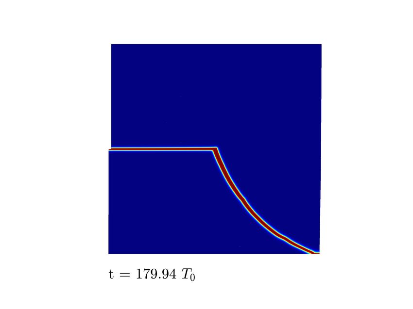
with bending modulus c and bαβ      αγ     βδ
                             0 := A bγδ A . Differentiating the Helmholtz free energy with
respect to metric and curvature components, yields the stress and moment components
                                                       ∂Ψ
                                            τ αβ   = 2      ,
                                                      ∂aαβ
                                                                                                (37)
                                                      ∂Ψ
                                            M0αβ   =      .
                                                     ∂bαβ

Here, these components are given with respect to the reference configuration but they can be
mapped to the current configuration by dividing the expressions in Eq. (37) by the surface
stretch J. The individual derivatives for the material model in Eqs. (34), (35) and (36) read
(Sauer and Duong, 2017; Zimmermann et al., 2019)
                                               αβ     αβ
                                   τ αβ     = τdil + τdev ,

                                    αβ        K 2
                                   τdil     =   (J − 1) aαβ ,
                                              2                                                 (38)
                                    αβ        G
                                   τdev     =    (2Aαβ − I1 aαβ ) ,
                                              2J
                                   M0αβ = c (bαβ   αβ
                                              0 − B ).

4.2.1   Split of the elastic energy density

Crack evolution shows anisotropic behavior since cracks will not propagate for every state of
stress. To avoid cracking in compression an energy split is required as follows

                                            Ψel = Ψ+     −
                                                   el + Ψel ,                                   (39)

where Ψ− el refers to the part of the elastic energy density that does not contribute to the fracture
process. Amor et al. (2009) make use of a split into deviatoric and dilational parts in which
crack evolution is not permitted in volumetric compression but allowed in states of volumetric
expansion and shear. In the work of Miehe et al. (2010a), a spectral decomposition of the strain
tensor is introduced in which only positive strains contribute to the fracture process. Likewise,
Kiendl et al. (2016) establish a spectral decomposition within a small deformation framework
in plates and shells. They outline that it is not possible to consider a split into tension and
compression as well as a split into membrane and bending contributions at the same time if
such a spectral decomposition of the total strain is used. In our formulation, the elastic energy
density is already split into membrane and bending parts according to Eq. (33) such that these
terms can be decomposed separately

                                          Ψ±     ±      ±
                                           el = Ψmem + Ψbend .                                  (40)

In the following, we show an example taken from Kiendl et al. (2016) that they use to motivate
the need for a thickness integration for the energy split. We use their example to motivate the
proposed split of the bending energy density. The strain distribution over the shell’s thickness
is illustrated in Fig. 2. The total strain Ẽ = E − ξK with components Ẽαβ and thickness
coordinate ξ ∈ − T2 , T2 can have both, positive and negative parts over the thickness T . It
follows that there is a region of compression, which must not contribute to the fracture process.
The membrane strains (due to the surface Green-Lagrange strain tensor E) are purely positive
in this example, whereas the strains associated with the curvature part are asymmetrically
distributed around the mid-plane of the shell. Since Kiendl et al. (2016) are only interested in the

                                                    10
tensile contributions, thickness effects for the elastic energy need to be considered to correctly
distinguish between tensile and compressive contributions to the total strain. In contrast to
this, the kinematical objects on the mid-plane include enough information for a suitable split of
the membrane part. Subsequently, the individual splits of in-plane and out-of-plane parts are
derived.
Ẽαβ Eαβ Kαβ T
2
+ +
ξ
= + +
− −
- T2
Figure 2: Strains over the shell’s thickness (Kiendl et al., 2016). In this example, the membrane
part shows purely positive strains, whereas the strains of the bending part are skew-symmetric
around the mid-plane. If the negative strains are not supposed to contribute to crack growth,
the strain distribution over the thickness has to be taken into consideration. Kiendl et al. (2016)
introduce a thickness integration and split the total strain with a spectral decomposition. Their
work motivates the necessity of our thickness integration (cf. Eq. (44)).
As already mentioned, a spectral decomposition of the strain tensor is not suitable in the
present formulation since our elastic energy density is given as a sum of membrane and bending
contributions. Instead, we follow the decomposition introduced by Amor et al. (2009), which
has also been used by e.g. Ambati et al. (2016) and Borden et al. (2016). Corresponding to
whether the surface stretch J is greater than/equal to 1 or smaller than 1, the dilatational part
will contribute to crack growth or not. The split of the membrane energy density required in
Eq. (40) then yields
( (
+ Ψdev + Ψdil , J ≥ 1 − 0, J ≥1
Ψmem = , Ψmem = . (41)
Ψdev , J 1). For instance Ambati et al.
(2015) shown that this split works well for fracture prediction, but we note that a suitable split
of the deviatoric energy density might be missing in Eq. (41).
The thickness has to be taken into account in order to obtain a suitable split of the bending
energy density in Eq. (36). This is obtained from following relation (Duong et al., 2017)
Z T
2
Ψbend = Ψ̃bend (ξ) dξ , (42)
− T2
where the corresponding three-dimensional constitutive model3 is given by
12 c 2
Ψ̃bend (K, ξ, T ) = ξ 2
tr K . (43)
T3 2
The split of Ψbend is then modeled as
Z T
2
Ψ±
bend = Ψ̃±
bend (ξ) dξ . (44)
− T2
3
This is a part of the Saint Venant-Kirchhoff model, see Duong et al. (2017).
11Still, Eq. (43) has to be additively decomposed according to Ψ̃bend = Ψ̃+ −
bend + Ψ̃bend . Already in
Eq. (41) the surface stretch at the mid-plane has been employed as an indicator for a possible
contribution to the fracture process. The surface stretch of other shell layers is obtained in
analogy to Eq. (12.2) as q
˜
J = det[Ãαβ ] det[ãαβ ] . (45)
The metrics Ãαβ and ãαβ follow from the tangent vectors Ãα and ãα of the shell layer at points
x + ξ n and X + ξ N , respectively (Duong et al., 2017). The split of Ψ̃bend then follows as
ξ 2 12 c tr K 2 , J(ξ)
˜ ≥1 0 , ˜ ≥1
J(ξ)
Ψ̃+
bend (ξ) = T 32 , Ψ̃−
bend (ξ) = 12 c . (46)
ξ 2 2 ˜The individual contributions in Eq. (50) are given in Eq. (38.2)-(38.3). The moment components
read
M0αβ = g(φ) M0,+ αβ αβ
+ M0,− , (51)
where the contributions are computed based on thickness integration via
Z T
2
αβ αβ
M0,± = M̃0,± (ξ) dξ , (52)
− T2
with
∂ Ψ̃bend (ξ) , 0 , ˜ ≥1
J(ξ)
˜ ≥1
αβ J(ξ) αβ
M̃0,+ (ξ) = ∂bαβ M̃0,− (ξ) = ∂ Ψ̃bend (ξ) . (53)
, ˜ 0. In our work we make use of a history field
H(x, t) := max Ψ+
el (x, τ ) , (55)
τ ∈[0,t]
which keeps track of the fracture contributing part of the elastic energy density (Miehe et al.,
2010a). Ψ+ el in Eq. (29) is then replaced by the history field H. Complex initial crack patterns
can also be realized by means of the history field (Borden et al., 2012). The history field
is often viewed as a driving force for fracture (Miehe et al., 2010a), but this viewpoint is
questionable, see Gerasimov and Lorenzis (2019). Also, the replacement of Ψ+ el by H violates
the variational nature of the formulation (Linse et al., 2017; Gerasimov and Lorenzis, 2019). The
new formulation with H is thus, not equivalent to the one with the original energy functional.
Despite the approximation of the irreversibility constraint, the new formulation leads to an easy
implementation and an easy introduction of initial cracks. Initial cracks can also be inserted as
discontinuities in the geometry. But this is more complicated in isogeometric discretizations,
than in standard finite element discretizations, especially for complicated initial crack patterns.
4.4 Euler-Lagrange equation and strong form
Combining Eqs. (28)–(29) and (55), the total energy in the system follows as
Z h i
Π := g(φ)H + Ψ− el + Ψ frac (φ) dA − Πext + Πkin . (56)
S0
13The kinetic energy Πkin and the potential energy Πext do not depend on φ. The elastic energy
density occurring from volumetric compression Ψ− el does not contribute to crack propagation
and is thus, not degraded in the domain of fracture. In contrast to this, H is degraded by
the degradation function g(φ), but is not a function of φ itself. Only the energy density Ψfrac
depends on φ, as seen in Eq. (30). The minimization of the energy functional can be expressed
by setting its variation to zero: δΠ = 0. The latter is solved by making use of the Euler-
Lagrange equation, which then leads to the strong form for the phase field’s evolution. Given
the Helmholtz free energy per reference area Ψ = Ψ(φ, φ,α , φ;αβ ), its variation reads
∂Ψ ∂Ψ ∂Ψ
δΨ = δφ + δ(φ,α ) + δ(φ;αβ ) . (57)
∂φ ∂φ,α ∂φ;αβ
Integration over the reference surface and applying integration by parts twice, yields
Z Z !
∂Ψ ∂Ψ ∂Ψ
δΨdA = − + δφ dA + boundary terms . (58)
S0 S0 ∂φ ∂φ,α ,α ∂φ;αβ ;αβ
The boundary terms vanish by choosing appropriate boundary conditions. Boundary conditions
for φ are given in Eq. (63). The energy minimization problem now reads δΨ = 0. Since Eq. (58)
holds true for all δφ, the Euler-Lagrange equation follows from applying the fundamental lemma
of variational calculus, yielding
∂Ψ ∂Ψ ∂Ψ
− + = 0. (59)
∂φ ∂φ,α ,α ∂φ;αβ ;αβ
Inserting the Helmholtz free energy per reference area described in Sec. 4 yields the strong form
of the phase field fracture equation
2`0 0
g (φ) H + φ − 1 − 2 `20 Aαβ φ;αβ + `40 Aγδ Aαβ φ;αβ ;γδ = 0 ,
∀φ ∈ S , (60)
Gc
with g 0 (φ) = ∂g(φ)/∂φ.
4.5 Weak form for the phase field fracture equation
Integrating Eq. (57) over the domain S0 , the weak form for the phase field fracture equation
becomes
Z Z Z
2
δφ f (φ) dA + ∇S (δφ) · 2`0 ∇S φ dA + ∆S (δφ) `40 ∆S φ dA = 0 , ∀ δφ ∈ V , (61)
S0 S0 S0
with
2`0 0
f (φ) := g (φ)H + φ − 1 , (62)
Gc
and the space of suitable test functions V = δφ ∈ H2 S(φ, t) . The boundary terms arising
during the derivation of Eq. (61) vanish due to the choice of the following boundary conditions
∆S φ = 0 ,
(63)
∇S `40 ∆S φ − 2`20 φ · n = 0 ,
for all φ(x, t) with x ∈ ∂S.
145 Discretization of the coupled problem
This section presents the monolithic discretization of the coupled system consisting of the thin
shell equation, the phase field evolution equation, and their interaction. For the numerical
examples presented in Sec. 6, the shell surface is discretized by isogeometric finite elements
(Hughes et al., 2005) since the high order operators of the coupled weak form require at least
global C 1 -continuity. For the spatial discretization, LR NURBS (Zimmermann and Sauer, 2017)
are employed to construct locally refined meshes in the domain of fracture. For the temporal
discretization, the generalized-α scheme of Chung and Hulbert (1993) is used.
5.1 Adaptive local surface refinement
5.1.1 LR NURBS
The fundamental work of Dokken et al. (2013) and their introduction of LR B-splines has been
extended to LR NURBS by Zimmermann and Sauer (2017). A knot vector Ξ of size n + p + 1
defines n linearly independent basis functions of order p. In the framework of LR NURBS,
the global knot vector Ξ = [ξ1 , ..., ξn+p+1 ] is split into local knot vectors Ξi = [ξi , ..., ξi+p+1 ]
(i = 1, . . . , n) to represent local parameter domains. Each of these local knot vectors defines a
single basis function. By construction the basis function has minimal support on the local knot
vector. Local refinement is performed by mesh line extensions in the parameter space. This
includes insertion of new mesh lines, joining or elongation of existing ones or an increase of their
multiplicity. The latter results in a decrease of continuity. Local refinement is based on knot
insertion (Dokken et al., 2013), which is described for LR NURBS in the work of Zimmermann
and Sauer (2017). LR NURBS inherit several mathematical properties from standard NURBS:
The basis forms a partition of unity, it is non-negative and the geometry lies within the convex
hull of the control points.
5.1.2 Criteria for surface refinement
An accurate phase field approximation of the discontinuity across the crack is achieved by using
a small length scale parameter `0 . This requires a highly resolved finite element mesh in the
vicinity of the crack. The phase field φ is used as an indicator for refinement: As soon as a
control point’s phase field value is smaller or equal to φbound , all elements that lie in the support
domain of the corresponding basis functions will be flagged for refinement. If these elements are
not yet refined up to a prescribed refinement depth, mesh line extensions are performed until the
desired refinement depth is achieved. The latter can be computed based on the element areas.
This refinement strategy is called Structured mesh (Johannessen et al., 2014) and is illustrated
in Fig. 3. The blue shaded area in the parameter domain resembles the support domain of a
basis function that is flagged for refinement. The dashed red lines are then inserted into the
parameter domain. This is done recursively for all newly created basis functions up to the
prescribed refinement depth. The refinement based on mesh line insertion and modification is
described in Sec. 5.1.1. We have found φbound = 0.975 to be a suitable choice for the threshold.
We note that in the case of crack nucleation, the last time step needs to be recomputed to
ensure crack initiation in a region of highly resolved mesh. But in case of crack propagation,
the last time step does not need to be resolved. Since the threshold value φbound is set very
close to the undamaged state, where φ = 1, the region around the crack tip is always refined
up to the highest prescribed refinement depth. The physically limited crack tip velocity and
15the chosen minimum time step size (see. Sec. 5.5.2) prevents the crack from propagating into
regions of coarser elements within one time step.
555
4
3
2
1
000
000 1 2 3 4 5 666
Figure 3: Refinement strategy Structured mesh: The blue shaded area resembles the support
domain of a basis function that is flagged for refinement. The dashed red lines are then inserted
into the parameter domain. (Johannessen et al., 2014)
5.2 Spatial discretization of primary fields
Subsequently, the finite element approximations of the surface deformation and the phase field
are described. It follows the work of Sauer et al. (2014), Sauer et al. (2017), Duong et al.
(2017) and Zimmermann et al. (2019). Let ne denote the number of spline basis functions
on parametric element Ωe . They are numbered with global indices i1 , . . . , ine . The surface
representation follows from this as
X h = N Xe , and xh = N xe , (64)
for the reference and current surface, respectively. The corresponding shape function array
reads
N := [Ni1 1, Ni2 1, ..., Nine 1] . (65)
Here, the element-level vectors are denoted Xe and xe and 1 refers to the (3×3) identity matrix.
Likewise, the phase field is approximated via
φh = N̄ φe , (66)
with element-level nodal values φe and shape function array
N̄ := [Ni1 , Ni2 , ..., Nine ] . (67)
The local vectors contain the nodal values with indices i1 , . . . , ine . These can be extracted from
the global ones X, x and φ which contain all nodal values. In analogy to Eqs. (64) and (66),
the corresponding variations read
δX h = N δXe , and δxh = N δxe , (68)
and
δφh = N̄ δφe . (69)
16Based on Eq. (64), the discretized tangent vectors follow as
Ahα = N,α Xe , and ahα = N,α xe , (70)
with N,α := ∂N/∂ξ α . From this, the discretized normals nh and N h follow according to
Eq. (4).4 The metric and curvature tensor components in the reference configuration are then
given by
Ahαβ = XT T
e N,α N,β Xe ,
h = Nh · N
and Bαβ ,αβ Xe , (71)
and similarly for the current surface
ahαβ = xT T
e N,α N,β xe , and bhαβ = nh · N,αβ xe . (72)
From this, the contra-variant metrics [Aαβ h −1 and [aαβ ] = [ah ]−1 follow. In analogy,
h ] = [Aαβ ] h αβ
the discretized variations of the surface metric and curvature are given by
δahαβ = δxT T T and δbhαβ = δxT T h
e N,α N,β + N,β N,α xe , e N;αβ n , (73)
with
N;αβ := N,αβ − Γγαβ N,γ , (74)
and discretized Christoffel symbols (cf. Sec. 2.1)
Γγαβ = xT T γδ
e N,αβ ah N,δ xe . (75)
Using Eqs. (7), (8) and (66), the derivatives of the phase field follow as
φh;α = N̄,α φe ,
∇S φh = Aαh N̄,α φe ,
∇S δφh = Aαh N̄,α δφe , (76)
∆S φh = ∆S N̄ φe ,
∆S δφh = ∆S N̄ δφe ,
with Aαh = Aαβ h α
h Aβ and N̄,α := ∂ N̄/∂ξ and
∆S N̄ := Aαβ ˆ (77)
h N̄;αβ ,
where
ˆ γ
(78)
N̄;αβ = N̄,αβ − Γ̂αβ N̄,γ .
Note that here, the discretized Christoffel symbols need to be taken from the reference surface
(cf. Sec. 2.1), i.e.
Γ̂γαβ = XT T γδ
e N,αβ Ah N,δ Xe . (79)
5.3 Spatial discretization of the mechanical weak form
Inserting the above approximations into Eq. (24) yields the discretized mechanical weak form
δxT fkin + fint − fext = 0 , ∀ δx ∈ U h ,
(80)
4
To avoid confusion, we write discrete arrays, such as the shape function array N, in roman font, whereas
continuous tensors, such as the normal vector N , are written in italic font.
17with global force vectors fkin , fint and fext . These are assembled from their respective elemental
contributions
Z
e
fkin := me ẍe , me := ρ NT N da ,
Ω e
Z Z
αβ αβ
e
fint := h T h
g(φ ) σ+ + σ− N,α aβ da + g(φh ) M+αβ + M−αβ N;αβ
T
nh da , (81)
Ωe Ωe
Z Z
e :=
fext NT p(φ) nh da + NT f α ahα da .
Ωe Ωe
αβ
The terms σ± and M±αβ are given by the energy split outlined in Sec. 4.2.1. In fext
e we have
taken the boundary loads T and M acting on ∂S as zero. The extension to boundary loads
e depends
can be found in Duong et al. (2017). Apart from the dependence on xe , the force fint
αβ
on φe through the degradation of σ+ and M+αβ by g(φh ).
From a physical point of view, the load-bearing capability vanishes in fully damaged regions
where φ = 0. Thus, no pressure can act on the corresponding regions. We account for this by
scaling the pressure linearly based on the phase field, i,.e.
p(φ) = φ p̄ , (82)
with p̄ denoting the pressure imposed on undamaged elements. Huge deformations and distorted
elements at regions of full damage are prevented by means of the pressure function in Eq. (82).
Putting everything together, the resulting equation system for the free nodes5 reads
f (x, φ) = M ẍ + fint (x, φ) − fext (x, φ) = 0 . (83)
The global mass matrix M is assembled from the elemental contributions me .
5.4 Spatial discretization of the phase field
Inserting the approximations from Sec. 5.2 into the discretized weak form of Eq. (61) yields
δφT f̄kin + f̄int − f̄ext = 0 , ∀ δφ ∈ V h ,
(84)
where the global vectors f̄kin , f̄int and f̄ext follow from the assembly of their corresponding
elemental contributions
e := 0 ,
f̄kin
Z
T
e
f̄int := k̄e0 φe + f̄ele − f̄0e , k̄e0 := N̄ N̄ + N̄T 2 αβ
,α 2`0 A N̄,β + ∆S N̄T `40 ∆S N̄ dA ,
Ωe0
Z
2`0 0
f̄ele := N̄T g (φ)H dA , (85)
Ωe0 Gc
Z
f̄0e := N̄T dA ,
Ωe0
e := 0 .
f̄ext
Apart from the dependence on φe , these expressions depend on xe through H. The resulting
equations at the free nodes simplify to
f̄ (x, φ) = f̄int (x, φ) = 0 . (86)
5
The free nodes refer to the degrees of freedom, which are not given by boundary conditions.
185.5 Temporal discretization
5.5.1 Generalized-α method
The fully implicit generalized-α method of Chung and Hulbert (1993) is used as a monolithic
time integration scheme. Given the quantities (xn , ẋn , ẍn , φn ) at time tn , the new values
(xn+1 , ẋn+1 , ẍn+1 , φn+1 ) at time tn+1 need to be found. Additionally, equilibrium has to be
fulfilled at intermediate states (xn+αf , ẋn+αf , ẍn+αm , φn+1 ), i.e.
" #
f xn+αf , ẍn+αm , φn+1
= 0. (87)
f̄ xn+αf , φn+1
The complete scheme has been described in the work of Zimmermann et al. (2019). Since there
are no temporal derivatives of the phase field in our framework, the corresponding equations
simplify as outlined in Appendix A. As shown for instance in Heister et al. (2015) and Gerasimov
and Lorenzis (2016), a monolithic coupling of the shell and phase field evolution equation
leads to a non-convex optimization problem. While in their work, a stabilization scheme or
a convexification of the energy functional is employed, we do not encounter any numerical
instabilites in our implicit time integration scheme. This is a result of the spatial and temporal
adaptivity approach. The first ensures a highly refined mesh around the crack tip, see Sec. 5.1.2,
while the adaptive time stepping scheme (presented subsequently) provides sufficiently small
time steps in case of crack propagation, see the numerical examples in Sec. 6. The combination
always ensured good convergence behavior, similar to the model presented by Borden et al.
(2012).
5.5.2 Adaptive time-stepping
The time step size should be chosen sufficiently small so that the crack does not propagate
across too many elements in one time step. In contrast to this, large time steps can be used
in cases of no crack propagation. This motivates the adaptive adjustment of the time step
size. Since the phase field is not time-dependent, we cannot apply the adaptive time stepping
scheme from Zimmermann et al. (2019). We therefore follow the subsequent approach: The
need for smaller or the possibility of larger time steps can be indicated by the required number
of Newton-Raphson iterations nNR during the last iteration, as for instance done by Schlüter
et al. (2014). We adjust the new time step size at time step n + 1 as
1.5 ∆tn , nNR < 4
1.1 ∆t , n = 4
n NR
∆tn+1 = . (88)
0.5 ∆t n , n NR > 4
0.2 ∆t , local spatial refinement
n
The coefficients in Eq. (88) have been chosen based on the numerical examples presented in
Sec. 6. Note that the time step size is also reduced after each spatial refinement step to ensure
good convergence behavior. If not specified otherwise, a maximum time step size ∆tmax =
0.1 T0 and the initial time step size ∆t0 = 1.5 · 10−5 T0 are used for the numerical results6 . In
the following numerical examples, we have observed that time step sizes smaller than 10−8 −
10−7 lead to ill-conditioned stiffness matrices. The maximum time step size has been mainly
determined based on numerical investigations and set in a way, such that the cracks do not
6
T0 refers to a reference time used to obtain a dimensionless formulation, see Sec. 5.7
19propagate over too many elements within one time step. We note that the latter can also be
determined based on the stress wave propagation speeds or the natural frequencies of the system
(Borden et al., 2012), also see Sec. 6.2.
5.6 Stabilization of jump conditions
In Eqs. (46) and (52) and in the corresponding linearizations (cf. Appendix B), integrals of the
form Z T (
2 ˜ ≥1
1, J(ξ)
ξ 2 χ J(ξ)
˜ ˜
dξ , with χ J(ξ)
= , (89)
− T2
˜5.7 Dimensionless form
The preceding formulation is normalized by introduction of the reference length L0 , surface
density ρ0 7 and time T0 . The corresponding dimensionless quantities are
x ρ t
x? = , ρ? = , t? = . (91)
L0 ρ0 T0
The normalization quantities for the in-plane material parameters K and G, the bending mod-
ulus c and the critical energy density Gc then follow as
K G c Gc
K? = , G? = , c? = , Gc? = , (92)
E0 E0 E0 L0 E0 L0
where E0 := ρ0 L20 T0−2 has units [N/m]. The surface stress σ αβ , the surface moment M αβ , the
surface tension γ, the elastic energy density Ψ and potential Π are then given by
σ αβ M αβ γ Ψ Π
σ?αβ = , M?αβ = , γ? = , Ψ? = , Π? = . (93)
E0 E0 L0 E0 E0 E0 L20
The temporal and spatial derivatives are (Zimmermann et al., 2019)
∂ ... ...
= T0 , ∇?S = L0 ∇S , ∆?S = L20 ∆S . (94)
∂t? ∂t
In the following, the superscript ? will be omitted for notational simplicity.
6 Numerical examples
This section shows several numerical examples of the proposed phase field formulation of brittle
shells. The material parameters of the elastic energy density (cf. Sec. 4.2) are given via
Eν E
K= , G= , c = 0.1 E0 L0 , (95)
(1 + ν) (1 − 2ν) 2 (1 + ν)
with stiffness E and Poisson’s ratio ν. For all subsequently presented results, bi-quadratic LR
NURBS are used and numerical integration on the bi-unit parent element is performed using
Gaussian quadrature with 3×3 quadrature points. Numerical thickness integration is performed
using four Gaussian quadrature points. For the visualization, the surface tension
1
γ = Nαα , (96)
2
is plotted, where Nαα are the mixed components from the stress occurring in the equation of
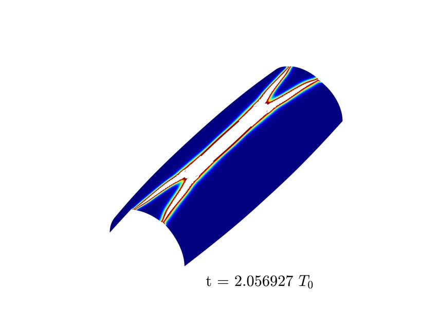
motion (18). All crack patterns are illustrated as follows: Red color resembles the fractured
state (φ = 0) and blue color indicates undamaged material (φ = 1). In between these states, a
transition based on the colors yellow-green-cyan is used.
Remark: The examples in this section exhibit stress waves. The present formulation does
not consider any damping such that stress waves do not dissipate but continue to propagate
and reflect. An artificial damping, e.g. based on energy absorbing boundary elements, could
be employed. Alternatively, physical viscosity can be introduced in the system, similar as is
done by Zimmermann et al. (2019). The challenge for the latter is to correctly split the viscous
7
Note that ρ0 is the surface density and has units [kg/m2 ].
21terms in analogy to the elastic split outlined in Sec. 4.2.1. Especially, the propagation of stress
waves over elements of different size needs to be investigated further. Stress waves can be
emitted from the crack, where the mesh is finest. As they cross mesh interfaces (where elements
of different sizes meet), it can happen that very fine waves are not represented on the coarse
mesh. It can be expected that for high loading intensities, these mesh interfaces thus lead to
unintentional and unphysical reflections of stress waves that may affect the fracture pattern. For
a physically correct assessment realistic damping formulations are needed. The development of
such formulations along with the investigation of stress waves is subject of future work.
6.1 2D shear test
The first example investigates crack evolution in a square two-dimensional membrane that is
exposed to a shear load. The geometry including boundary and loading conditions is illustrated
in Fig. 5. The mesh is initially constructed from 16 × 16 LR NURBS elements and the region
ū
0.5L0
initial crack
0.5L0
0.5L0 0.5L0
Figure 5: 2D shear test: Specimen geometry, boundary and loading conditions.
next to the initial crack is refined by LR NURBS elements up to a refinement depth of d = 5, see
Fig. 7. The material parameters are given in Tab. 1. The initial phase field distribution, which
E [E0 ] ν [−] ∆ū [L0 ] Gc [E0 L0 ] `0 [L0 ] T [L0 ]
100 0.2 2· 10−6 0.001 0.0025 0.0125
Table 1: 2D shear test: Material parameters and imposed load increment ∆ū per time step.
is induced by an initial history field, and the crack evolution are shown in Fig. 6. The crack
evolves towards the bottom right corner on a curved path. The qualitative behavior resembles
the results shown in the literature. For instance, in Borden et al. (2012) a quasi-static two-
dimensional shear test has been investigated where the crack path has been locally refined a
priori based on analysis-suitable T-splines.
Our results show that the split of the membrane energy from Sec. 4.2.1 works correctly since no
branch is forming towards the specimen’s top edge. Based on the adaptive spatial refinement
strategy from Sec. 5.1.2, the LR mesh is refined as the crack evolves. The parametric domains
of the LR meshes are illustrated in Fig. 7. Only the regions of damage are refined up to the
prescribed refinement depth d = 5, while the periphery is kept coarse. Fig. 8 shows the time
step sizes employed and the contributions to the total energy in the system. The latter have
22You can also read