Volume Statistics as a Probe of Large-Scale Structure
←
→
Page content transcription
If your browser does not render page correctly, please read the page content below
Volume Statistics as a Probe of Large-Scale Structure

                                                                                     Kwan Chuen Chan(1)∗ and Nico Hamaus(2)
                                                                              1
                                                                               School of Physics and Astronomy, Sun Yat-sen University,
                                                                                 2 Daxue Road, Tangjia, Zhuhai, 519082, China and
                                                                                2
                                                                                  Universitäts-Sternwarte München, Fakultät für Physik,
                                                                       Ludwig-Maximilians Universität, Scheinerstr. 1, 81679 München, Germany
                                                                                                (Dated: January 29, 2021)
                                                               We investigate the application of volume statistics to probe the distribution of underdense regions
                                                            in the large-scale structure of the Universe. This statistic measures the distortion of Eulerian
                                                            volume elements relative to Lagrangian ones and can be built from tracer particles using tessellation
                                                            methods. We apply Voronoi and Delaunay tessellation to study the clustering properties of density
                                                            and volume statistics. Their level of shot-noise contamination is similar, as both methods take into
arXiv:2010.13955v2 [astro-ph.CO] 28 Jan 2021

                                                            account all available tracer particles in the field estimator. The tessellation causes a smoothing
                                                            effect in the power spectrum, which can be approximated by a constant window function on large
                                                            scales. The clustering bias of the volume statistic with respect to the dark matter density field is
                                                            determined and found to be negative. We further identify the Baryon Acoustic Oscillation (BAO)
                                                            feature in the volume statistic. Apart from being smoothed out on small scales, the BAO is present
                                                            in the volume power spectrum as well, without any systematic bias. These observations suggest
                                                            that the exploitation of volume statistics as a complementary probe of cosmology is very promising.

                                                                  INTRODUCTION                                   correlations with other more abundant tracers, such as
                                                                                                                 galaxies [44] or clusters [47, 48], are considered. Another
                                                  Modern large-scale structure surveys probe both the            option is the use of overlapping spherical voids, as demon-
                                               background expansion and the growth of structure, which           strated by Ref. [43] in the measurement of the BAO in the
                                               can be used to constrain the energy content of the Uni-           void auto-correlation function. Allowing voids to overlap
                                               verse and help resolve the mystery behind the cosmic              increases their number density by up to two orders of
                                               expansion [1]. These surveys have been remarkably suc-            magnitude, but the signal-to-noise ratio of the resulting
                                               cessful in constraining the parameters in ΛCDM and its            clustering statistic is more difficult to interpret.
                                               extensions [2–9]. Because most observed galaxies trace               In practice voids are identified via sparse tracers, as
                                               the high-density regions of the Universe [10], previous           the full mass distribution cannot be observed directly in
                                               analyses typically focus on the clustering statistics of          all three dimensions. Since many tracers are needed to
                                               overdensities. However, the dominant part of the Uni-             define a single void, the resulting void distribution is even
                                               verse exhibits a low density compared to its mean value.          more sparse. Therefore, the question arises whether one
                                               The clustering of underdensities may therefore contain            can construct a field estimator for the low-density regions
                                               additional information that is complementary to that ob-          with low level of shot noise and without overlap. The vol-
                                               tained via conventional methods.                                  ume statistic proposed in this paper satisfies these con-
                                                  Cosmic voids are extended regions of relatively low            ditions. In Sec. , we define the volume statistic in detail.
                                               matter content in the large-scale structure, they are po-         In order to implement it in data, we need to estimate the
                                               tentially ideal proxies for studying the underdense parts         density field using tessellation methods. We briefly re-
                                               of the Universe [11–13]. Because of their unique envi-            view two tessellation interpolation methods and contrast
                                               ronment, interesting phenomena such as the dark energy            them with the conventional mass assignment scheme in
                                               [14–17], modified gravity [18–22], and the influence of           Sec. . The possibility of approximating its impact on the
                                               massive neutrinos [23–26] become more visible in voids.           power spectrum by an effective window is discussed in
                                               Recently, there have been numerous studies on the clus-           Sec. . Sec. is devoted to studying the overall clustering
                                               tering of voids using samples derived from cosmological           properties of the volume statistic, such as the bias pa-
                                               surveys, exploiting effects such as Redshift-Space Distor-        rameter and the BAO feature. We conclude in Sec. . In
                                               tions (RSD) in the void-galaxy correlation function [27–          the appendices, we review the the Kernel Density Esti-
                                               35], the Alcock-Paczynski test [36–41], and the Baryon            mation method (Appendix ) and the effects of a window
                                               Acoustic Oscillations (BAO) [42, 43]. However, the spa-           function on the power spectrum (Appendix ).
                                               tial number density of voids is generally low due to their
                                               large size; hence their auto-clustering statistic exhibits
                                               a considerable shot noise contribution [44–46]. While                              VOLUME STATISTICS
                                               small voids are more abundant, they actually reside in
                                               regions of higher density (so-called voids-in-clouds [13]),         Voids are extended underdense regions in the Universe
                                               only larger voids truly trace the underdense regime of            and it has been shown that they furnish a biased tracer of
                                               large-scale structure. To mitigate the shot noise, cross-         the large-scale structure [13, 25, 44, 49–53]. Small voids
2

tend to reside in overdense environments and therefore         where δL and δh are the halo density contrast in La-
exhibit positive bias parameters; they are in the so-called    grangian and Eulerian space, respectively. However, in
void-in-cloud regime [13]. Large voids, on the contrary,       observations we have no direct access to δL . One practi-
are anti-correlated with overdense structures and thus         cal way to bypass this difficulty is to define J as
exhibit a negative clustering bias [44], i.e. they trace
large-scale underdensities (it is interesting to note that                                 d3 x         1
                                                                                 J ≡             3
                                                                                                    =                        (5)
the quadratic bias of voids follows a similar trend to that                            (1 + δL )d q   1 + δh
of halos [52]). However, their number density is signifi-
                                                               even for the case of halos. We can think of it as the
cantly lower than that of small voids (owing to their size),
                                                               volume change inversely weighted by the halo density in
which results in a high shot-noise contribution and hence
                                                               Lagrangian space.
a low signal-to-noise ratio of their large-scale auto-power
                                                                  The advantage of the volume statistic is as follows.
spectrum. In this work, instead of defining single objects
                                                               First, it is a fundamental measure of the volume change
from a large number of tracers, we assign a volume to
                                                               induced by the large-scale structure evolution. From
each individual tracer particle, which helps to mitigate
                                                               a theoretical perspective it is likely more amenable to
the shot noise.
                                                               models than the statistics of voids, which are defined by
   In the Lagrangian picture of large-scale structure, we
                                                               the complicated nonlinear topology of the cosmic web.
can think of each tracer particle carrying a volume ele-
                                                               In the linear regime the volume statistic reduces to the
ment that is being distorted over time. This evolution is
                                                               one of linear density fluctuations. In the weakly non-
governed by mass conservation, and for the case of dark
                                                               linear regime it can be treated with perturbation theory
matter we have [54]
                                                               or other analytic methods. Second, the volume statistic
                      d3 q = (1 + δ)d3 x,               (1)    makes use of all the available tracer particles, resulting in
        3         3
                                                               a shot-noise level comparable to its original tracer field.
where d q and d x are the volume elements in the La-           Nevertheless, because the majority of particles are lo-
grangian (initial) and Eulerian (evolved) space, respec-       cated inside collapsed regions, the sampling is still poor
tively, and δ is the matter density contrast in Eulerian       compared to the conventional density statistic. On the
space. Then we define                                          other hand, because of the denominator 1 + δ, V is un-
                            d3 x    1                          defined when δ = −1. This can pose problems in the
                      J ≡        =     .                (2)    density estimation for sparse samples, such as massive
                            d3 q   1+δ
                                                               halos. We will therefore consider tessellation methods to
J is the Jacobian of the transformation from the La-           avoid such singularities.
grangian coordinate q to the Eulerian coordinate x. It            The volume statistic up-weights underdense regions
quantifies the change in volume compared to that in the        and down-weights overdense ones; hence it is similar to
Lagrangian space. When the displacement is small, J            certain types of marked correlation functions in spirit1 .
reduces to 1 − δ with a symmetric distribution around          If each particle is assigned a mark m, the marked corre-
a mean equal to 1. For large displacements and hence           lation M for the mark can be generally defined as [59]
nonlinear δ, J has a mean larger than 1 and the distri-
bution becomes skew symmetric with a singular tail at                                         1     X
                                                                                 M (r) =              mi mj ,                (6)
δ = −1. This indicates that inside empty regions in Eule-                                         2
                                                                                           N (r)m̄ ij
rian space, a tremendous amount of expansion in volume
has occurred. After shell crossing, the volume element         where N (r) is the total number of pairs with separation
d3 q can split into multiple parts and the fluid description   r and m̄ is the mean of the mark. The mark can be
by Eq. (1) is no longer valid. Nonetheless, shell cross-       chosen to highlight any particular physics of interest. For
ing occurs mainly in the high-density regions, which are       example, [60] proposed to consider a mark of the form
down-weighted in J , and hence its impact on our statis-                                          p
tic is minimal.                                                                           ρ∗ + 1
   In analogy to the density contrast, we can define the                         m=                   ,                (7)
                                                                                        ρ∗ + 1 + δ
volume statistic as
                   J         1                                 where ρ∗ and p are free parameters. This mark has been
               V ≡ ¯ −1= ¯         − 1,                 (3)    applied to study modified gravity [61]. If we set ρ∗ = 0
                   J     J (1 + δ)
                                                               and p = 1, it reduces to the volume statistic. However,
where J¯ is the mean of J . For small δ, it reduces to −δ.     the value of ρ∗ is often taken to be order unity, e.g. in [61],
  For halos the situation is more complicated, because         so as to avoid the singularity problem mentioned above.
the density is no longer uniform in Lagrangian space,
and we have instead (e.g. [55, 56])
               (1 + δL )d3 q = (1 + δh )d3 x,           (4)    1   This can be generalized to the marked power spectrum [57, 58].
3
Moreover, the definition of the volume statistic is sim- CIC it is a top-hat, and for TSC it is a triangular-shaped
ilar to the log-transform of the density field [62] cloud centered on the particle position. In fact these are
the first three members of an infinite hierarchy of interpo-
A = log(1 + δ). (8) lating functions that can be generated via iterative con-
volution with the top-hat window function [64]. In NGP
It was found that the field A is more Gaussian than δ the particle mass is interpolated to the nearest grid point,
at late times, and some higher-order information in δ is in CIC the mass is assigned to the grid points of the cell
pulled back into the two-point statistics of A [62, 63]. enclosing the particle (8 points in 3D), and the particle
Both transformations up-weight the low-density regions mass is interpolated to the neighboring 27 points in TSC.
and down-weight the high-density ones. In fact, both Thus, the window becomes more extended as the order
the log-field and the volume statistic diverge at δ = −1. of the interpolation scheme increases. Because the win-
The log-transform aims to recover the information in the dow function is a constant linear operator, its effect can
initial density field, as it accommodates both the low- be removed by division of W in Fourier space. To repre-
density and the high-density regions. Our goal is less sent the density field for clustering analyses, the grid size
ambitious and we merely want to recover the information is usually chosen sufficiently large to mitigate resolution
from the underdense regions. By restricting our target, effects3 . Among the mass-interpolation methods, CIC is
it is easier to define a density reconstruction method that the most common one, so we use it as our benchmark.
suits precisely this purpose.
INTERPOLATION METHODS Tessellation interpolation
In order to compute the volume statistic one needs a The tessellation method can generate a space-filling
density estimate that is finite everywhere. To this end we field with finite values (non-vanishing) everywhere in con-
use interpolation by tessellation to reconstruct the den- figuration space; it is often used as an intermediate step
sity field from a discrete particle distribution. As this to obtain a smooth density field and to define extended
type of method is rarely used directly for clustering anal- structures in the cosmic web, e.g. [67–73]. However, it
yses, we shall first compare it against the commonly used has rarely been used directly for clustering analyses of
mass interpolation method. the density field. Given a set of points (generators) xα , a
tessellation generates cells that are space-filling and mu-
tually disjoint [74, 75]. Applications of the tessellation
Mass interpolation methods in cosmology were introduced in [75–80].
In the Voronoi tessellation, each Voronoi cell encloses
For the large-scale clustering analysis, the density one generator and every point x belongs to a Voronoi cell
field is often interpolated to a grid2 . The interpolation Vα if the distance |x−xα | is smaller than |x−xβ | for any
methods usually employed include Nearest Grid Point other β. The simplest possibility is to assume that the
(NGP), Cloud-in-Cell (CIC), and Triangular-Shaped particle mass spreads out uniformly within a Voronoi cell
Cloud (TSC). We collectively denote them as mass- and the density within each cell is estimated by the mass
interpolation methods, they are discussed extensively in of the particle and the volume of the Voronoi cell. This
the monograph [64]. In these methods, particles are method yields a piece-wise constant field and the field
smoothed by a window function (or cloud function) W of value is discontinuous across the boundaries. We shall
fixed size and these windows can overlap with each other. refer to the technique to estimate densities in this way as
The density at the grid point xp is given by the Voronoi Tessellation Field Estimator (VTFE).
XZ To obtain a continuous field we can tessellate the space
ρ(xp ) = d3 x W (x − xα ), (9) into Delaunay cells. In 3D, a triangulation divides space
α [xp ] into tetrahedrons. A Delaunay tessellation is such a tri-
angulation with the additional property that the circum-
where [xp ] denotes the grid cell enclosing xp and the sum sphere of each tetrahedron does not contain any gener-
is over all the particles. ators. The field value inside a tetrahedron can then be
The three-dimensional (3D) window can be con-
structed from its 1D form as W (x) = W (x)W (y)W (z).
In 1D, the NGP window function is the Dirac delta, for
3 Discrete sampling of the continuous field introduces aliasing ef-
fect [64–66], which is especially serious for modes close to the
Nyquist frequency. We are limited to the large-scale modes be-
2 The configuration-space estimation of correlation functions uses cause of the tessellation interpolation, we shall not consider it
counting of pairs directly without the need for a grid. here.4
obtained by linear interpolation from the vertices. Ex- Poisson sample the underlying density field4 . The den-
plicitly, the number density at a point x inside a Delau- sity estimated by smoothing the particle distribution is
nay cell with vertices x0 , x1 , x2 , and x3 , is given by [75] akin to the kernel density estimation (KDE) method in
statistics, which is used to estimate the probability den-
n(x) = n(x0 ) + (x − x0 )i J −1iα ∆nα , (10) sity distribution (see e.g. [83]). In Appendix , we review
the KDE and show that given a sample of particles it can
where ∆nα indicates the difference in density between be used to estimate the number density of the sample, n
vertex xα and the reference vertex x0 , n(xα ) − n(x0 ). A [Eq. (45)]. In particular, it is shown that smoothing in-
Latin index denotes the spatial component of the vector troduces a bias to the density estimate [Eq. (46)]. At a
and a Greek index represents the vertex (also from 1 to peak (trough) of the density field, the window-estimated
3). The Jacobian J is the transformation matrix between density field is biased low (high). However, the advantage
the coordinate x and the barycentric coordinate ζα of smoothing the density field is that it can suppress the
variance of the estimator [Eq. (47)]: it is inversely pro-
∂xi portional to the average volume of the window size. In
Jiα = ≈ (xα − x0 )i . (11)
∂ζα statistics, the mean squared error, which is a sum of the
variance and the bias squared, matters if the signal-to-
The number density at the generator can be estimated noise ratio of the measurement is not high. Thus the
by [75, 80] KDE is useful if its suppression to the variance is larger
than its bias.
1+D For the case of density estimation by tessellation, the
n(xα ) = P , (12)
Vadj (xα )
adj
Dx
density at the position x depends on the particles span-
α
ning the cell. It is hard to make an analytic estimate of
where D is the dimension of space, Dxadj denotes all the its bias and variance, because of the irregular shape of
α
adjacent Delaunay cells with xα as one of their gener- the cell and the interpolation scheme depending on all
ators, and Vadj is the volume of the adjacent Delaunay the points in the cell. For the case of VTFE, because
cells. This construction ensures that the integral of the there is only one generator inside a Voronoi cell, we can
density field obtained from Eq. (10) is equal to the to- write down the density estimate as (N = 1)
tal particle mass. We refer to this method of estimating 1
x − xα
the density as the Delaunay Tessellation Field Estimator n̂VTFE (x) = 3 WVTFE , (13)
hα hα
(DTFE) in this paper.
Effectively, tessellation methods smooth out the par- where WVTFE describes the Voronoi cell around a point
ticle mass adaptively based on the local density. For x, xα is the generator of the Voronoi cell, and hα
high-density regions, the effective window size is small, schematically represents the characteristic size of the cell.
while it is large in the low-density regime. For the mass- Because the Voronoi cell is generally not symmetric
interpolation methods, such as the CIC, as the size of about its generator, the bias reads
the grid increases the resulting density field approaches
a sum of Dirac delta distributions. Thus, this method
X (1) ∂n h2 X ∂ 2 n (1)
hn̂(x)i − n(x) = −hα Ii + α I ,
can produce the same type of distribution as the point i
∂xi 2 ij ∂xi ∂xj ij
set. On the other hand, the tessellation method aims at (14)
reconstructing a smooth (piecewise constant for VTFE
and continuous for DTFE) density field from the discrete where the function I is defined in general in Eq. (40). In
particle distribution. This additional requirement intro- particular, because of the irregular shape of the Voronoi
duces a smoothing to the small-scale power spectrum. cells, I (1) is in general non-vanishing. However, if we
The smoothing scale is dictated by the mean particle now further average over the shape of the Voronoi cell
(1)
separation of the distribution. In summary, in the mass- WVTFE , hIi i vanishes and we obtain
interpolation scheme, the effective window-function size
is controlled by the grid size, while that of the tessellation hh2α i X ∂ 2 n (1)
hn̂(x)i − n(x) = hI i. (15)
method is determined by the mean particle separation. 2 ij ∂xi ∂xj ij
Similar to the standard KDE case [Eq. (46)], we recover
Effects of the tessellation: An analytic estimate the result that the bias is sourced by the second deriva-
In the mass-interpolation scheme, a fixed window is
4
used to smooth the particle distribution. An analytic In the case of halos and voids there are exclusion effects that
estimate can be made if the particles are assumed to violate this assumption [44, 49, 81, 82]5
tives of the density. The variance of the estimator reads Each simulation consists of a cubic box of 1000 Mpc h−1
x − x side length and contains 5123 particles. The Gaussian
1 α initial conditions are generated by CLASS [84] at redshift
Var(n̂(x)) = 6 Var WVTFE
hα hα z = 49. In order to study the BAO signature, we ran an-
I (2) other set of simulations with Einsenstein-Hu initial con-
≈ n(x). (16) ditions without the BAO wiggles [85] (NoWiggle). The
h3α
particle displacements are implemented using 2LPTic [86]
Further averaging over the shape of the Voronoi cell, we and are evolved with the N -body code Gadget2 [87]. Ha-
have los are identified using the halo finder AHF [88]. They are
defined via a spherical overdensity threshold of 200 times
1
Var(n̂(x)) = hI (2) in(x). (17) the background density and contain at least 20 particles.
h3α For each simulation set, 20 realizations are used. The re-
For DTFE, the density at x [Eq. (10)] depends on the sults derived from the halo samples will be our primary
position of the vertices nonlinearly and the previous an- interest in this paper. We shall illustrate our results us-
alytic arguments do not apply. Nonetheless, we shall see ing four halo samples at z = 0 and 1, with two sets of
that the features of the DTFE are qualitatively similar initial conditions, respectively. Unless otherwise stated,
to those of the VTFE. the error bars are the standard error of the mean of the
measurements among all realizations.
The procedures for density estimation using the tes-
EFFECTIVE WINDOW FUNCTION sellation method are similar to those in the public code
DTFE [89], which implements the density estimation by
In this section we investigate whether the effects of the Delaunay tessellation efficiently. We implement both
the tessellation can be modeled by an effective window Voronoi and Delaunay tessellation methods using the
function. The width of the window involved in the mass python libraries based on the Qhull code [90]. After
interpolation is controlled by the grid size, which can be generating the tessellation cells we use a cubic grid to es-
chosen such that the grid effects are negligible, or the win- timate the density at the grid points, which can then be
dow function effect can be divided out in Fourier space. used for the estimation of power spectra. We use a grid
Hence we may treat the density field obtained from the size of 2563 and average over 23 uniformly spaced sam-
CIC, δCIC , as the unsmoothed field for comparison. pling points within each grid cell to calculate the mean
In Appendix we review the effects of the window func- density at the grid point. We have checked that these
tion on the power spectrum. We show that if the particle choices are sufficiently accurate for our results.
distribution is smoothed by a constant window function
W , the effect on the power spectrum is captured by an Measurement of the effective window
overall factor of |W |2 (or W for the case of cross-power
spectrum). Note that the same window function factor
We measure the effective window function of the tessel-
applies to both the continuous clustering and the shot-
lation using random catalogs and halo samples. Without
noise term. Thus, if the effective window function can be
intrinsic clustering it is easier to identify the impact of
taken to be a non-stochastic function, the power spec-
the effective window on the power spectrum, since the
trum of the density field obtained with the tessellation
remaining clustering amplitude is simply white noise. To
method, δtess , can be written as5
generate the random catalogs, particle positions are ran-
hδtess (k)δtess (k0 )i = (2π)6 |Wtess (k)|2 hδCIC (k)δCIC (k0 )i. domly placed in a cubic box of size 1000 Mpc h−1 until the
(18) desired number density is reached (we match it with the
Similarly for consistency, the cross-correlation is given by halo sample density). Assuming that halos Poisson sam-
ple the underlying continuous density field, the shot-noise
hδtess (k)δCIC (k0 )i = (2π)3 Wtess (k)hδCIC (k)δCIC (k0 )i. contribution to their power spectrum is given by [91]
(19)
1
We test these relations using simulation data, the de- Pshot = , (20)
tails of which are described in the following. The as- (2π)3 n̄
sumed cosmology is a flat ΛCDM model with parameters where n̄ is the mean halo density. We show in Ap-
Ωm = 0.3, ΩΛ = 0.7, h0 = 0.7, ns = 0.967, and σ8 = 0.85. pendix that there is an additional factor of |W |2 , if the
particle distribution is smoothed by a window W .
The effective VTFE window obtained using Eqs. (18)
5
and (19) from the random catalog is shown in Fig. 1. In
The Fourier convention used in this paper is
R d3 x −ik·x this case the CIC power spectrum is given by Eq. (20).
f (x) and f (x) = d3 keik·x f (k).
R
f (k) = (2π) 3e
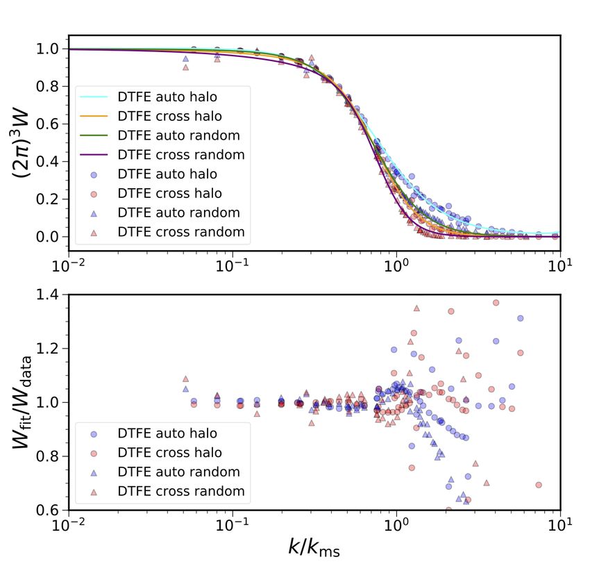
The size of the effective window can be characterized by6
FIG. 1. Top: the VTFE effective window function measured FIG. 2. As Fig. 1, but for the DTFE results.
from the random catalog (triangles) and the halos (circles).
Measurements from the auto-power spectrum (blue) and the
cross-power spectrum (red) are shown. The fits using Eq. (21)
are over-plotted (cyan for Wa from halos, green for Wa from
Ptess /PCIC and Ptess,CIC /PCIC , with Ptess and PCIC being
randoms, orange for Wc from halos and purple for Wc from
randoms). Bottom: the ratio between the fits and the mea- the halo auto-power spectra obtained with the tessella-
surements (circles for halos and triangles for randoms, blue tion and the CIC method, and Ptess,CIC the cross-power
for auto- and red for cross-power spectra). spectra between them. Note that we have not subtracted
shot noise in any of those cases. The curves from halo
samples are somewhat less universal than for the ran-
the mean separation wavenumber kms ≡ πn̄1/3 . We find doms, especially at high q. This is expected, as the halos
that using the variable q ≡ k/kms , the effective window exhibit intrinsic clustering that is scale dependent, mak-
obtained from different tracers falls on a universal curve. ing their effective window more extended due to stronger
Thus, kms represents the characteristic size of the tessel- clustering on smaller scales.
lation cell in Fourier space6 . Although the window from
We find that the overall window function shape can be
the auto- and cross-power spectra (denoted as Wa and
described well by the functional form
Wc , respectively) agree with each other at low k, Wa is
more extended than Wc . In fact, Wc turns negative at
q ∼ 1.8, while Wa remains positive everywhere. Eqs. (18) 1
(2π)3 W (q) = , (21)
and (19) imply that we can extract the same window (1 + aq)[1 + (bq)n ]
function from the auto- and cross-power spectrum mea-
surements. However, in practice, this only works on large
scales, so the assumption that W (k) factorizes and does with q = k/kms .
not explicitly depend on the density field δ(k) must fail We have shown the best-fit values obtained from the
on smaller scales. VTFE and the DTFE in Table I. The results for the halo
Even if the particle distribution is intrinsically clus- and random samples obtained with Wa and Wc are com-
tered, the window function still factors out. In Fig. 1 we pared. These best fits are also plotted in Figs. 1 and
also show the effective window function extracted from 2. Up to q . 1, the accuracy of the fit is about 10%
within the scatter of the data. As there are significant
differences between Wa and Wc , obtaining a universal
fit that is accurate at q & 1 is not possible. Overall,
6 We note that in Lagrangian space, the typical extension of halo the DTFE results are in qualitative agreement with the
density profiles is controlled by halo mass. When the density
profile is rescaled by this characteristic extension, most of the
VTFE ones. However, we find that the measurements of
mass dependence is removed and the halo density profiles fall on WDTFE are slightly more extended than WVTFE . This
a rather universal curve [92]. Thus, kms is analogous to the role implies that the DTFE window is more compact in con-
of mass for Lagrangian halos. figuration space.7
1.2 z = 1, M = 1.7 × 10 M h 1.2 z = 1, M = 1.1 × 10 M h
13 1 14 1
TABLE I. The best-fit parameters for Eq. (21) for the VTFE
and DTFE methods. The results derived from Wa and Wc
for the random and halo samples are shown. 1.1 1.1
P(k) ratio
VTFE random VTFE halo DTFE random DTFE halo
1.0 1.0
Wa Wc Wa Wc Wa Wc Wa Wc
VTFE Wa halo
a 0.09 0.50 -0.08 0.37 0.07 0.37 -0.09 0.20 0.9 VTFE Wc halo 0.9
VTFE Wa random
b 1.49 1.36 1.55 1.35 1.36 1.29 1.37 1.28 VTFE Wc random
0.8 0.8
n 2.47 3.94 2.08 3.14 2.75 4.18 2.20 3.25 10 2 10 1 10 2 10 1
1.2 z = 0, M = 1.8 × 10 13 M h 1
1.2 z = 0, M = 1.6 × 10 14 M h 1
1.1 1.1
P(k) ratio
Power spectrum ratio 1.0 1.0
0.9 0.9
After having measured the effective window functions
0.8 0.8
of the tessellation methods, we are now in the position 10 2 10 1 10 2 10 1
to test whether we can use this window to recover the k/ Mpc 1h k/ Mpc 1h
unsmoothed power spectrum. We utilize the ratio
FIG. 3. Auto-power spectrum ratio Eq. (22) from the VTFE
window for Wa (blue) and Wc (red) from the halo (circles) and
X
Ptess random (triangles) samples. The mean mass and redshift of
[(2π)3 W (k)]n − Pshot the halo samples are shown on top of each panel.
R= , (22)
PCIC − Pshot
1.2 z = 1, M = 1.7 × 10 M h 1.2 z = 1, M = 1.1 × 10 M h
13 1 14 1
to quantify the accuracy of this reconstruction, where
1.1 1.1
X denotes auto- (n = 2) or cross-power spectra (n =
P(k) ratio
1). In Fig. 3 we show the ratio R for the auto-power 1.0 1.0
spectrum using the VTFE windows Wa and Wc from halo
DTFE Wa halo
and random samples. For the rest of this paper, we will 0.9 DTFE Wc halo 0.9
DTFE Wa random
exclusively show the results based on these four samples. DTFE Wc random
0.8 0.8
At low k, Wa appears to yield a better agreement than 10 2 10 1 10 2 10 1
Wc . However, inspection of Fig. 1 reveals that this can 1.2 z = 0, M = 1.8 × 10 13 M h 1
1.2 z = 0, M = 1.6 × 10 14 M h 1
be explained by the fact that Wc is a bit lower than Wa
at small q. This is an artifact of the fitting formula. 1.1 1.1
P(k) ratio
On the other hand, when k is close to kms , the ratio
deviates substantially from 1. A division by the window 1.0 1.0
function is prone to noise and systematic error, which 0.9 0.9
become inflated at high k when W is small. Even if we
use Wc from a direct measurement, the pattern at high 0.8 0.8
k in R remains unchanged. Also, the trends are very 10 2 10 1 10 2 10 1
similar for both the halo and the random samples. In
k/ Mpc 1h k/ Mpc 1h
Fig. 4 we show the corresponding results for the DTFE,
which are qualitatively similar to the VTFE case. The FIG. 4. As Fig. 3, but for the DTFE results.
ratios using the cross-power spectra in Eq. (22) are very
similar, so we do not show them here.
CLUSTERING OF THE VOLUME FIELD
Our results suggest that approximating the tessellation
with a constant effective window function is valid on large
scales, but above kms the density-dependent nature of the The shot noise of the volume field
tessellation method is important and smoothing effects
cannot be removed by division of a window function. In We estimate the shot noise of the volume field PVn
this case, it is necessary to determine the tessellation- using the random catalog again and showcase the auto-
smoothed density field numerically. power spectra of the volume statistic before and after8
z = 1, M = 1.7 × 10¹³ M h 1, VTFE z = 1, M = 1.7 × 10¹³ M h 1, DTFE
CIC random CIC halo /w SN CIC random CIC halo /w SN
103 VTFE random VTFE halo /w SN 103 DTFE random DTFE halo /w SN
CIC halo /w SN VTFE halo CIC halo /w SN DTFE halo
P(k) 102 102
101 101
100 100
10 2 10 1 10 2 10 1
z = 0, M = 1.8 × 10¹³ M h 1, VTFE z = 0, M = 1.8 × 10¹³ M h 1, DTFE
103 103
102 102
P(k)
101 101
100 100
10 2 10 1 10 2 10 1
k/ Mpc 1h k/ Mpc 1h
FIG. 5. Auto-power spectra of the volume statistic before (triangles) and after shot-noise subtraction (circles) for the VTFE
(left panels, red) and the DTFE (right panels, green). The conventional halo-density power spectra are shown for comparison
(blue), along with the shot noise contamination estimated from the randoms (stars). The vertical dashed line indicates the
mean tracer separation scale kms and the horizontal one shows the Poisson power spectrum Pshot . The mean mass and redshift
of the halo samples are shown on top of each panel. On large scales, the shot-noise level of the volume field is comparable to
that of the halo sample used to construct it.
shot noise subtraction in Fig. 5. Although the volume spectra, Phh and Phm ,
statistic is obtained via nonlinear transformation of the
halo tracer field, on large scales the shot noise still ap- r
Phh − Phn
proaches Pshot as given by Eq. (20). However, it is sup- bhh = , (23)
Pmm
pressed by the effects of the tessellation on smaller scales.
Phm
After shot noise is subtracted from the power spectra, bhm = , (24)
the results from the VTFE and DTFE agree with the Pmm
shot-noise subtracted CIC case. Thus, since all available
tracer particles are used to construct the volume field, its where Pmm denotes the matter auto-power spectrum and
shot-noise contamination is indeed similar to that of the Phn is the halo shot noise contribution obtained from the
original tracer field. random catalog. As a comparison, we also show bhh and
bhm obtained from the CIC method.
On large scales the density-bias parameter obtained via
The bias of the volume field the tessellation methods approaches the one obtained via
the CIC mass assignment, which already reaches a con-
The volume field can be regarded as a biased tracer of stant value at k . 0.08 Mpc−1 h. On smaller scales, the
the underlying dark matter density field. As it traces the bias parameter from the tessellation is damped by the
underdense regions of large-scale structure, we expect it effective window function, as discussed in the previous
to exhibit a negative clustering bias, similar to large voids section. The differences between bhh and bhm are appar-
[13, 44, 49]. To guide our interpretation of the volume ent for k & 0.1 Mpc−1 h. Consistent with the findings
statistic, we first investigate the bias of the more com- in Sec. , Fig. 6 shows that the DTFE window is more
mon density field obtained via the tessellation method compact than the VTFE window in configuration space.
in Fig. 6. We compare the bias parameters bhh and bhm To fit the large-scale bias function, the scale dependence
derived from the halo auto- and halo-matter cross-power of the window must be taken into account and a possible9
z = 1, M = 1.7 × 10¹³ M h 1, VTFE z = 1, M = 1.7 × 10¹³ M h 1, DTFE
2.5
2 2.0
1.5
b 1 1.0
0.5
0
10 2 10 1 10 2 10 1
z = 0, M = 1.8 × 10¹³ M h 1, VTFE z = 0, M = 1.8 × 10¹³ M h 1, DTFE
1.00 bhh fit CIC 1.00 bhh fit CIC
bhm fit CIC bhm fit CIC
0.75 bhh fit VTFE 0.75 bhh fit DTFE
bhm fit VTFE bhm fit DTFE
b
0.50 bhh CIC 0.50 bhh CIC
bhm CIC bhm CIC
0.25 bhh VTFE bhh DTFE
bhm VTFE 0.25 bhm DTFE
10 2 10 1 10 2 10 1
k/ Mpc 1h k/ Mpc 1h
FIG. 6. The clustering bias of the halo density field obtained with the CIC, VTFE (left
panels), and DTFE (right panels) methods. The measurements originate from the halo auto-
power spectrum, bhh (CIC: grey stars, VTFE: red triangles, DTFE: green triangles) and the
halo-matter cross-power spectrum, bhm (CIC: black stars, VTFE: red circles, DTFE: green
circles). The fit using Eq. (25) is over-plotted, dashed for bhh and solid for bhm ; cyan, orange,
and purple for CIC, VTFE, and DTFE measurements, respectively. Redshifts and mean halo
masses are indicated on top of each panel. On large scales, the bias measurements obtained
with the tessellation methods are in good agreement with the CIC ones.
z = 1, M = 1.7 × 10¹³ M h 1, VTFE z = 1, M = 1.7 × 10¹³ M h 1, DTFE
0 0
1 1
b
2 2
10 2 10 1 10 2 10 1
z = 0, M = 1.8 × 10¹³ M h 1, VTFE z = 0, M = 1.8 × 10¹³ M h 1, DTFE
0.0 bhm fit CIC 0.0 bhm fit CIC
b fit VTFE b fit DTFE
b m fit VTFE b m fit DTFE
0.5 bhm CIC
b VTFE
0.5 bhm CIC
b DTFE
b
b m VTFE b m DTFE
1.0 1.0
10 2 10 1 10 2 10 1
k/ Mpc 1h k/ Mpc 1h
FIG. 7. As Fig. 6, but for the clustering bias of the volume field V. To compare with the
magnitude of the conventional halo-density bias, the negative of bhm is shown. The properties
of the halo samples used to construct the volume statistics are indicated on top of each panel.
The bias of the volume field is negative and its magnitude is similar to that of the halo sample.10
functional form is a quartic polynomial similar gains can be expected, but with a lower level of
2 4 shot-noise contamination. One can think of the volume
b(k) = c0 + c2 k + c4 k , (25)
field as a “dual” of the density field with negative bias
where c0 , c2 , and c4 are the fit parameters. In Fig. 6 within the same survey volume. Thanks to their very
we have also plotted the best-fit curves, using modes up different bias amplitudes, but comparable shot-noise lev-
to kmax = 0.06 Mpc−1 h, yielding a good agreement with els, the density and volume fields together may provide
the simulation data. optimal conditions for conducting a multi-tracer analysis
We now turn to the bias of the volume field, presented [97–99].
in Fig. 7. The auto- and cross-bias for the volume field Although bVm is not directly observable in galaxy sur-
is defined in analogy to Eqs. (23) and (24), veys, this can be circumvented by considering
r
PVV − PVn PhV
bVV = − , (26) bhV = , (28)
Pmm Pmm
PVm
bVm = , (27)
Pmm where PhV is the observable cross-power spectrum be-
tween δh and V. The dark matter power spectrum Pmm
with PVV being the auto-power spectrum of the volume
can be modeled numerically or using perturbation theory.
field and PVm the cross-power spectrum between the vol-
On large scales, where the fluctuations are small and the
ume field and the matter density field. The shot noise
bias is linear, we have bhV ≈ bhm bVm . In Fig. 8 we plot
of the volume field PVn is estimated using the random
the bhV measurement from our simulation. We note that
catalog again. Note that because the volume field anti-
since the volume field is constructed from the halos, there
correlates with the dark matter density field, its bias is
is a residual correlation analogous to the standard shot
negative. To ease comparison with the magnitude of the
noise in the halo auto-power spectrum. We measure the
halo bias, we have also shown −bhm . The overall shape
cross-power spectrum between the density field and the
of the bias functions of the volume field is similar to the
volume field obtained from the random catalog with the
density ones. On large scales, the bias of the volume field
same number density as the halo field and subtract it
approaches the halo bias in magnitude. This is expected
from PhV . Both the results before and after this shot-
for large-scale fluctuations that are small, since in that
noise subtraction are shown. We indeed find that the
limit V reduces to −δh . However, although bVm agrees
shot-noise subtracted results are in good agreement with
with the halo bias well, there is a marked deviation of
the prediction bhm bVm , for which we have used the fit
bVV from the former. We presume there to be loop cor-
results from bhm and bVm obtained with Eq. (25).
rections to the power spectrum of quadratic order in den-
sity, analogous to the shot-noise renormalization effect in
the local bias case ([93], see also [63]). These additional
shot-noise-like contributions cause deviations from the The BAO in the volume field
linear bias on large scales. On small scales, the density
field is suppressed by the tessellation and the definition In the early Universe, photons and baryons couple
of V is designed such that it approaches zero in the limit to form a hot plasma in which acoustic oscillations are
of vanishing δh . Hence, the behavior of the bias of V excited. These oscillations leave important imprints in
is qualitatively similar to that of the tessellation density large-scale structure of the late Universe [100, 101]. The
field. BAO features are regarded as one of the most impor-
Like cosmic voids, the volume field furnishes a nega- tant probes of the large-scale structure and have been
tively biased tracer of large-scale structure. Although the detected in numerous galaxy surveys [1].
small-scale power is suppressed by the tessellation, the Physically, the BAO manifests itself as an excess prob-
large-scale field is proportional to the underlying den- ability of finding galaxies at a distance rd , the sound
sity field. In scenarios involving local primordial non- horizon at the drag epoch. This appears as a peak at the
Gaussianity (PNG), the void bias exhibits a scale de- scale rd in the galaxy density correlation function and
pendence on large linear scales [51]. Because the am- as oscillations (wiggles) in Fourier space. Analogously,
plitude of void bias can be negative, this may be used given a depression of V at some location, it is more likely
to complement the traditional halo bias in constraining to find another depression of V at a distance of rd . This
PNG [94]. Ref. [51] demonstrated that a combination of also gives rise to a positive enhancement in the corre-
halos and voids, taking advantage of the so-called multi- lation function of V at the scale of rd . We now go on
tracer approach [95, 96], allows to substantially tighten to investigate the anticipated BAO signals in the volume
constraints on the non-Gaussianity parameter fNL . How- statistic in more detail. To do so we use two sets of sim-
ever, the gain in the constraining power of that analysis ulations, one with the fiducial setup, and another one
is limited by the shot noise in void auto-clustering statis- with the Eisenstein-Hu initial conditions without BAO
tics. As the volume field also exhibits a negative bias, wiggles [85].11
z = 1, M = 1.7 × 10¹³ M h 1, VTFE z = 1, M = 1.7 × 10¹³ M h 1, DTFE
2.5 2.5
b 0.0 0.0
2.5 2.5
5.0 5.0
10 2 10 1 10 2 10 1
z = 0, M = 1.8 × 10¹³ M h 1, VTFE z = 0, M = 1.8 × 10¹³ M h 1, DTFE
1 1
bh VTFE bh DTFE
0 bhm CIC
b m VTFE
0 bhm CIC
b m DTFE
b
bh VTFE w/ SN bh DTFE w/ SN
bh VTFE bh DTFE
1 1
10 2 10 1 10 2 10 1
k/ Mpc 1h k/ Mpc 1h
FIG. 8. The clustering bias bhV obtained from the cross-power spectrum between the halo density field and the volume field
using the VTFE (left panels, red) and the DTFE (right panels, green) methods. Because the volume field is derived from
the halo distribution, there is a shot-noise contribution. Both the results before (triangles) and after shot-noise subtraction
(squares) are compared. The halo bias bhm (black stars) and volume bias bVm (VTFE: red circles, DTFE: green circles) are
shown for reference. The solid curves (cyan for VTFE and orange for DTFE) are the predictions obtained using the fit results
from Eq. (25), which are in good agreement with the direct measurements.
Real space that there is smoothing of the ratio between the wiggle
and no-wiggle power spectrum implies that the smooth-
ing effect cannot be attributed to a constant window and
We begin with the BAO features measured in the real-
it must arise from the density-dependent nature of the
space density field using the tessellation methods. To
tessellation methods. Numerous works have shown that
highlight the BAO features, we show the ratio between
the nonlinearity of density fields causes a smoothing of
power spectra from the fiducial and the no-wiggle initial
the BAO and its effect on the power spectrum can be
conditions in Fig. 9. The results for different halo groups
approximated by a Gaussian window [55, 102–104]. This
obtained with three interpolation methods are compared.
damping of the BAO is primarily driven by the large-
The BAO feature in the dark matter field is also shown
scale bulk flow motion. Because the tessellation methods
for reference, which is determined with the CIC method.
adaptively track the evolution of the particle distribu-
The number density of dark matter particles is so high
tion, the associated window has a similar effect, resulting
that its density field can be regarded as continuous here.
in a smoothing of the BAO wiggles. This interpretation
On large scales (small k) all methods produce similar on the tessellation window is consistent with results in
results, as the large-scale modes are unaffected by the in- Sec. .
terpolation methods. At higher k (compared to kms ), the
CIC halo field is still able to reproduce the BAO features We now turn to the BAO imprints in the volume field,
imprinted in the dark matter density field, albeit with as presented in Fig. 10. The BAO measurement in the
more noise. On the other hand, for the VTFE and DTFE volume field is noisier than that in the density. In par-
fields the BAO wiggles start to be smoothed out close to ticular, although the VTFE and DTFE behave similarly
kms and are suppressed significantly at k & kms . Follow- for the density case, the DTFE yields more noisy results
ing Appendix , when the particle distribution is smoothed than the VTFE for the volume field. Overall, the BAO
by a constant window function, the window factors out wiggles imprinted in the volume field follow those in the
and cancels in the power spectrum ratio. Thus, the fact matter density field without any systematic bias. As in12
1.15 z = 1, M = 1.7 × 10¹³ M h 1 1.15 z = 1, M = 1.1 × 10¹⁴ M h 1
CIC
1.10 VTFE 1.10
DTFE
1.05 DM 1.05
P/PNoWigg 1.00 1.00
0.95 0.95
0.90 0.90
0.85 0.85
0.00 0.05 0.10 0.15 0.20 0.25 0.30 0.00 0.05 0.10 0.15 0.20 0.25 0.30
1.15 z = 0, M = 1.8 × 10¹³ M h 1 1.15 z = 0, M = 1.6 × 10¹⁴ M h 1
1.10 1.10
1.05 1.05
P/PNoWigg
1.00 1.00
0.95 0.95
0.90 0.90
0.85 0.85
0.00 0.05 0.10 0.15 0.20 0.25 0.30 0.00 0.05 0.10 0.15 0.20 0.25 0.30
k/ Mpc 1h k/ Mpc 1h
FIG. 9. Ratio between real-space halo density power spectra from simulations with fiducial and no-wiggle initial conditions.
The results for different halo density fields obtained with the CIC (blue), VTFE (red), and DTFE (green) method are shown.
The corresponding measurements from the dark matter (black solid curve) are overplotted as reference. The vertical dashed
line indicates the mean separation scale kms of the halos. The halo density power spectra from the tessellation methods can
reproduce the BAO features on large scales, while the power beyond kms is suppressed.
z = 1, M = 1.7 × 10¹³ M h 1 z = 1, M = 1.1 × 10¹⁴ M h 1
1.1 1.1
P/PNoWigg
1.0 1.0
CIC
VTFE
0.9 DTFE 0.9
DM
0.00 0.05 0.10 0.15 0.20 0.25 0.30 0.00 0.05 0.10 0.15 0.20 0.25 0.30
z = 0, M = 1.8 × 10¹³ M h 1 z = 0, M = 1.6 × 10¹⁴ M h 1
1.1 1.1
P/PNoWigg
1.0 1.0
0.9 0.9
0.00 0.05 0.10 0.15 0.20 0.25 0.30 0.00 0.05 0.10 0.15 0.20 0.25 0.30
k/ Mpc 1h k/ Mpc 1h
FIG. 10. As Fig. 9, but for the volume field constructed from the halo distribution. The black curve shows the BAO from the
dark matter density field. The blue data points are the CIC measurement of the modified V statistic with = 0.1. On large
scales, the volume statistics computed with the tessellation methods exhibit BAO features without systematic bias.13
the density case above, beyond kms the BAO signature is are similar to the real-space case. The halo monopole
washed out. from the CIC interpolation appears to trace the wiggles
In the standard CIC interpolation, V is ill-defined for in the dark matter monopole power spectrum well. While
regions with δh = −1, which happens for empty grid cells. the tessellation results are slightly less noisy than the
To overcome this problem, we can instead define CIC ones for k < kms , they are suppressed for k & kms .
Fig. 12 displays the monopole power spectrum for the
1
J = , (29) volume statistics. As in real space, V yields the most
1 + δh + noisy estimator and the VTFE results are the most ro-
J bust in reproducing the dark matter BAO. We note that
V = ¯ − 1,
J the BAO amplitude in the volume field appears slightly
with some constant > 0, which ensures that V is always enhanced at some scales. This is particularly apparent
well-defined. We show the results for = 0.1 in Fig. 10. for the V estimator, which is most sensitive to noise. We
This method yields noisier results than the tessellation therefore attribute this effect to the discreteness of the
methods. We have checked that other values of , such tracer distribution.
as 0.01 or 0.2, do not improve this.
Redshift space Discussion
Observationally, we can only perform BAO measure- Besides the auto-power spectrum, we can measure the
ments in redshift space. As the coordinates of the galax- BAO using the cross-power spectrum between δh and V.
ies along the line-of-sight direction are deduced from red- The results are similar to those obtained from the auto-
shifts in galaxy surveys, the density field is subject to power spectrum on large scales, but they are more noisy
additional perturbations due to their peculiar motion. for k & kms , since the volume field lacks the BAO feature
These perturbations cause RSD, and we shall consider on small scales. So far we have exclusively investigated
them in the plane-parallel limit, with the comoving co- Fourier-space statistics. In configuration space, the ef-
ordinate in the z-direction xz modified to fect of the tessellation is a smoothing of the BAO peak
vz as well. Thus, the BAO feature measured from the corre-
sz = xz + (30)
aH lation function of the volume field is broadened and be-
comes less sharp, making it harder to differentiate from
where vz is the peculiar velocity in z-direction and H is
the broad-band correlation function.
the Hubble parameter. We can adapt Eq. (4) to redshift
space as In order to fully capture the BAO features in the power
spectrum of the volume statistics, the number density
∂x 3 of the tracer sample must be sufficiently high. For ex-
(1+δL )d3 q = 1+δh (x) d s = 1+δh (s) d3 s. (31)
∂s ample, at z = 0 the halo sample with mean mass 1.8 ×
Accordingly, we have 1013 M h−1 and number density 2.3×10⁻⁴ ( Mpc h−1 )−3
is sufficient. At higher redshift, the BAO wiggles are less
d3 s 1 damped by nonlinearities, so a higher number density is
J = = . (32)
3
(1 + δL )d q 1 + δh (s) necessary to push kms to a larger value. For instance,
at z = 1 the halo number density needs to be at least
Hence, the extension of the volume statistic to redshift 7 × 10⁻⁴ ( Mpc h−1 )−3 to fully capture the BAO wiggles.
space is straightforward.
To summarize the virtues of each method: for the den-
The redshift-space power spectrum can be expressed
sity statistics the CIC interpolation method is recom-
in terms of multipoles,
mended, as it offers an unbiased estimate of the small-
2` + 1 1
Z scale density field, while the VTFE and DTFE smooth
P` = dµPs (k, µ)L` (µ), (33) out the field for scales above kms . The tessellation im-
2 −1
poses additional conditions such that the resultant field is
where Ps is the power spectrum in redshift space, µ the smooth and space-filling. These requirements modify the
cosine of the angle between k̂ and the line of sight, and small-scale behavior of the field. On the other hand, in
L` is the Legendre polynomial of order `. Here we only order to exploit volume statistics the tessellation method
show results for the monopole of the halo power spec- is preferred, as it is able to construct a space-filling field
trum, as the quadrupole measurements are noisy even with non-vanishing density everywhere. The results from
for 20 realizations. the VTFE are similar to the DTFE for the density statis-
The monopole power spectrum for the halo density tics, but VTFE yields more robust results for the volume
field in redshift space is shown in Fig. 11. The results statistics. Another advantage of the VTFE is its lower14
z = 1, M = 1.7 × 10¹³ M h 1 z = 1, M = 1.1 × 10¹⁴ M h 1
CIC
1.1 VTFE 1.1
DTFE
P/PNoWigg DM
1.0 1.0
0.9 0.9
0.00 0.05 0.10 0.15 0.20 0.25 0.30 0.00 0.05 0.10 0.15 0.20 0.25 0.30
z = 0, M = 1.8 × 10¹³ M h 1 z = 0, M = 1.6 × 10¹⁴ M h 1
1.1 1.1
P/PNoWigg
1.0 1.0
0.9 0.9
0.00 0.05 0.10 0.15 0.20 0.25 0.30 0.00 0.05 0.10 0.15 0.20 0.25 0.30
k/ Mpc 1h k/ Mpc 1h
FIG. 11. As Fig. 9, but for the monopole power spectrum of the density statistics in redshift space. Similar to the results in
real space, apart from the smoothing for k & kms , the tessellation methods accurately reproduce the BAO wiggles in redshift
space.
z = 1, M = 1.7 × 10¹³ M h 1 z = 1, M = 1.1 × 10¹⁴ M h 1
1.1 1.1
P/PNoWigg
1.0 1.0
CIC
VTFE
0.9 DTFE 0.9
DM
0.00 0.05 0.10 0.15 0.20 0.25 0.30 0.00 0.05 0.10 0.15 0.20 0.25 0.30
z = 0, M = 1.8 × 10¹³ M h 1 z = 0, M = 1.6 × 10¹⁴ M h 1
1.1 1.1
P/PNoWigg
1.0 1.0
0.9 0.9
0.00 0.05 0.10 0.15 0.20 0.25 0.30 0.00 0.05 0.10 0.15 0.20 0.25 0.30
k/ Mpc 1h k/ Mpc 1h
FIG. 12. As Fig. 10, but for monopole power spectrum of the volume statistics in redshift space. Similar to the results in real
space, the large-scale BAO features are imprinted in the redshift-space volume power spectra without systematic bias.15
computational overhead compared to DTFE7 . Hence, for can be substantial overlap between the circumspheres of
the clustering analysis of volume statistics, we recom- neighboring tetrahedrons. In the void construction algo-
mend usage of the VTFE. rithm, the void center and size are determined entirely by
A measurement of the BAO feature from the distribu- the four particles spanning the tetrahedron. The point-
tion of underdense regions is interesting on its own, but like nature of the void-center position prevents any ad-
it may also provide valuable information on cosmology in ditional smoothing of the BAO; however, the resultant
addition to what is available from halo clustering alone. BAO measurement may be more correlated with the den-
We have demonstrated that the volume statistic traces sity statistic.
the large-scale structure with a negative bias parame- Finally we comment on the possible effects of the BAO
ter. What remains to be shown is how correlated the reconstruction [103]. BAO reconstruction is often ap-
volume statistic and the traditional halo density statis- plied in galaxy surveys (e.g. [106]) to undo part of the
tic are. Since the volume statistic is constructed via the large-scale gravitational evolution and RSD effect so as
halo tracer distribution, the answer is not obvious. For to boost the BAO signal. This is because the recon-
example, one can construct a trivial field −δh , which ex- structed field becomes more correlated with the initial
hibits negative linear bias8 , but perfectly correlates with conditions, so the BAO signal in the volume field is ex-
δh . In order to investigate the correlation between δh and pected to increase as well. For example, V reduces to
V, one could determine the covariance of the power spec- −δh for weak fluctuations and we expect the BAO signal
trum from both the density and the volume field using to be well correlated between these two fields. However,
many different realizations, which is beyond the scope of a detailed study is required to access the overall gain in
this paper. BAO information from the reconstructed volume field.
A simple (albeit less conclusive) test is to consider the
cross-correlation coefficient between δh and V
CONCLUSIONS
PhV
r= √ , (34)
Phh PVV In large-scale structure analyses it is common to ex-
where Phh , PVV , and PhV are the halo auto-, volume ploit statistics based on the galaxy distribution, which
auto-, and halo-volume cross-power spectra. predominantly traces high-density regions in the Uni-
The results for fields constructed from four different verse. However, a large fraction of its volume exhibits
halo groups are shown in Fig. 13. We have used the relatively low density. Hence, the clustering of under-
full redshift-space monopole power spectra including shot dense regions may bear cosmologically relevant informa-
noise. On large scales, both δh (estimated via CIC) and tion that is complementary to the conventional clustering
V (estimated via VTFE or DTFE) are (anti-) correlated of overdensities. In principle, cosmic voids are ideal prox-
with the dark matter δ and with each other, but due to ies for probing the underdense regions, but their auto-
the presence of shot noise and other sources of stochastic correlation statistics suffer a large shot-noise contamina-
noise in the volume field, r is slightly above −1. The tion due to their low number density. In this work we pro-
characteristic shape of the curve is due to the exclusion pose to apply the volume statistic V to probe the volume
between δh and V. At smaller scales, exclusion can lead distribution of large-scale structure. This statistic pro-
to oscillations before r approaches to zero, but they are vides a measure of the volume change between Eulerian
quickly suppressed when the shot noise kicks in at high and Lagrangian space. As it makes use of all the tracer
k. If the volume statistics were as trivial as −δh , r would particles available, its shot-noise level is similar to that
be equal to −1 on all scales. of the conventional tracer density field. Furthermore, the
We note that the BAO features are also detectable us- definition of the volume statistic is closely related to the
ing overlapping voids [42, 43], which are defined to be density contrast, so it may be more amenable to theoret-
the circumspheres of the tetrahedrons resulting from the ical models based on perturbation theory than objects
Delaunay tessellation of the galaxies [105]. Although this that are defined via nonlinear topological characteristics
approach is similar to ours in using the tessellation to par- of the cosmic web, such as voids. Also, an extension of
tition the point set, we do not define objects on it. There its definition to redshift space is straightforward.
Traditional mass-assignment methods, such as CIC in-
terpolation, yield empty regions with δh = −1 for sparse
halo samples, which make the volume statistic estimator
7 In a typical run with a single core on an Intel Xeon E5-2686 clus- ill-defined there. To overcome this difficulty, we apply
ter, the VTFE takes about 40 minutes, while the DTFE about tessellation interpolation methods to estimate the volume
24 hours. Perhaps the DTFE algorithm can be more efficient
after further optimization.
field. We study the clustering statistics obtained via the
8 However, for voids the behavior of quadratic bias is similar to tessellation methods in detail. The power spectrum from
that of halos [49, 52], so at second order the bias of this artificial the tessellated field is smoothed by an effective window
field is opposite to that of the genuine underdense tracer. function, which on large scales can be approximated byYou can also read