Gridded and direct Epoch of Reionisation bispectrum estimates using the Murchison Widefield Array
←
→
Page content transcription
If your browser does not render page correctly, please read the page content below
Publications of the Astronomical Society of Australia (PASA)
                                               doi: 10.1017/pas.2019.xxx.

                                               Gridded and direct Epoch of Reionisation bispectrum
                                               estimates using the Murchison Widefield Array
arXiv:1905.07161v1 [astro-ph.CO] 17 May 2019

                                               Cathryn M. Trott1,2∗, Catherine A. Watkinson3 , Christopher H. Jordan1,2 , Shintaro Yoshiura4 , Suman
                                               Majumdar5,3 , N. Barry11,2 , R. Byrne8 , B. J. Hazelton8,12 , K. Hasegawa4 , R. Joseph1,2 , T. Kaneuji4 ,
                                               K. Kubota4 , W. Li13 , J. Line1,2 , C. Lynch1,2 , B. McKinley1,2 , D. A. Mitchell10 , M. F. Morales8,2 ,
                                               S. Murray1,2,6 , B. Pindor11,2 , J. C. Pober13 , M. Rahimi11 , J. Riding11 , K. Takahashi4 , S. J. Tingay1 ,
                                               R. B. Wayth1,2 , R. L. Webster11,2 , M. Wilensky8 , J. S. B. Wyithe11,2 , Q. Zheng14 , David Emrich1 ,
                                               A. P. Beardsley6 , T. Booler1 , B. Crosse1 , T. M. O. Franzen12 , L. Horsley1 , M. Johnston-Hollitt1 ,
                                               D. L. Kaplan7 , D. Kenney1 , D. Pallot9 , G. Sleap1 , K. Steele1 , M. Walker1 , A. Williams1 , C. Wu9 ,
                                               1 International Centre for Radio Astronomy Research (ICRAR), Curtin University, Bentley WA, Australia
                                               2 ARC   Centre of Excellence for All Sky Astrophysics in 3 Dimensions (ASTRO 3D), Australia
                                               3 Department of Physics, Blackett Laboratory, Imperial College, London SW7 2AZ, United Kingdom
                                               4 Kumamoto University, Japan
                                               5 Centre of Astronomy, Indian Institute of Technology Indore, Simrol, Indore 453552, India
                                               6 School of Earth and Space Exploration, Arizona State University, Tempe, AZ 85287, USA
                                               7 Department of Physics, University of Wisconsin–Milwaukee, Milwaukee, WI 53201, USA
                                               8 Department of Physics, University of Washington, Seattle, WA 98195, USA
                                               9 International Centre for Radio Astronomy Research (ICRAR), University of Western Australia, Crawley, WA 6009, Australia
                                               10 CSIRO Astronomy & Space Science, Australia Telescope National Facility, P.O. Box 76, Epping, NSW 1710, Australia
                                               11 School of Physics, The University of Melbourne, Parkville, VIC 3010, Australia
                                               12 University of Washington, eScience Institute, Seattle, WA 98195, USA
                                               13 Brown University, Department of Physics, Providence, RI 02912, USA
                                               14 Shanghai Astronomical Observatory, China

                                               Abstract
                                               We apply two methods to estimate the 21 cm bispectrum from data taken within the Epoch of
                                               Reionisation (EoR) project of the Murchison Widefield Array (MWA). Using data acquired with
                                               the Phase II compact array allows a direct bispectrum estimate to be undertaken on the multiple
                                               redundantly-spaced triangles of antenna tiles, as well as an estimate based on data gridded to the uv-
                                               plane. The direct and gridded bispectrum estimators are applied to 21 hours of high-band (167–197 MHz;
                                               z=6.2–7.5) data from the 2016 and 2017 observing seasons. Analytic predictions for the bispectrum bias
                                               and variance for point source foregrounds are derived. We compare the output of these approaches, the
                                               foreground contribution to the signal, and future prospects for measuring the bispectra with redundant
                                               and non-redundant arrays. We find that some triangle configurations yield bispectrum estimates that
                                               are consistent with the expected noise level after 10 hours, while equilateral configurations are strongly
                                               foreground-dominated. Careful choice of triangle configurations may be made to reduce foreground bias
                                               that hinders power spectrum estimators, and the 21 cm bispectrum may be accessible in less time than
                                               the 21 cm power spectrum for some wave modes, with detections in hundreds of hours.

                                               Keywords: cosmology – instrumentation – Early Universe – methods: statistical

                                               1 INTRODUCTION                                                     distribution details of the radiation field and gas proper-
                                                                                                                  ties in the intergalactic medium permeating the cosmos
                                               Exploration of the growth of structure in the first billion        (Furlanetto et al., 2006; Pritchard & Loeb, 2008). Red-
                                               years of the Universe is a key observational driver for            shifted to low frequencies, the 21 cm line is accessible
                                               many experiments. One tracer of the conditions within              with radio telescopes (ν < 300 MHz), including current
                                               the early Universe is the 21 cm spectral line of neutral           and future instruments. These include the Murchison
                                               hydrogen, which encodes in its brightness temperature              Widefield Array, MWAi (Bowman et al., 2013; Tingay
                                                  ∗ cathryn.trott@curtin.edu.au                                      i http://www.mwatelescope.org

                                                                                                              1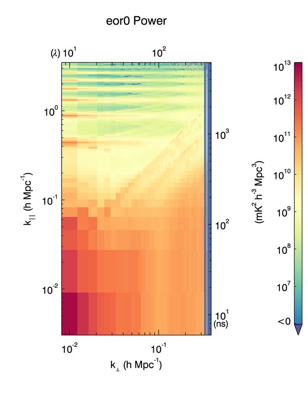
2                                                                                                            Trott et al.

et al., 2013; Jacobs et al., 2016); the Precision Array       case in the CMB community, where non-Gaussianities
for Probing the Epoch of Reionization, PAPERii (Par-          can be contaminated by structured foregrounds (Jung
sons et al., 2010); the LOw Frequency ARray, LOFARiii         et al., 2018).
(van Haarlem et al., 2013; Patil et al., 2016); the Long         Majumdar et al. (2018) explore the ability of the
Wavelength Array, LWAiv (Ellingson et al., 2009), and         bispectrum to discriminate fluctuations in the matter
the future HERA (DeBoer et al., 2016) and SKA-Low             density distribution from those of the hydrogen neutral
(Koopmans et al., 2015).                                      fraction, reporting that for some triangle configurations
   The weakness of the signal, combined with the expec-       the sign of the bispectrum is a marker for which of these
tation that most of its information content is contained      processes is dominating the bispectrum. They show out-
in the second moment (Wyithe & Morales, 2007), which          put bispectra for equilateral and isosceles configurations
is uncorrelated across spatial Fourier wave mode, mo-         over a range of wavemodes and redshifts, including pa-
tivates the use of the power spectrum as a statistical        rameters of relevance to current low-frequency 21 cm
tool for detecting and characterising the cosmological        experiments (z < 9, 0.1 < k < 1.0). For modes rele-
signal. Despite the ease with which the power spectrum        vant to the MWA, the bispectrum amplitude fluctu-
can be computed from radio interferometric data, the          ates in sign with wavenumber and triangle geometry
presence of strong, spectrally-structured residual fore-      (stretched → equilateral → squeezed) with a range span-
ground sources (Trott et al., 2012; Datta et al., 2010;       ning 103 − 109 mK3 h−6 Mpc6 . This range of potential
Vedantham et al., 2012; Thyagarajan et al., 2015), com-       signs and amplitudes in measurable modes and redshifts,
plex instrumentation (Trott & Wayth, 2016), and imper-        motivates us to study this signal in MWA data.
fect calibration (Patil et al., 2014; Barry et al., 2016),       Watkinson et al. (2018) provide a useful tool for visu-
yield power spectra that are dominated by systemat-           alising the correspondence of real-space structures and
ics. Thus far, a detection of signal from the Epoch of        bispectrum. They highlight that equilateral k-vector
Reionisation has not been achieved (Patil et al., 2016;       configurations probe above-average signal concentrated
Beardsley et al., 2016; Trott et al., 2016; Cheng et al.,     in filaments with a circular cross section (their Figure
2018). These systematics, combined with the expecta-          1). Stretched (flattened) k-vector triangle configurations
tion that non-Gaussian information can be extracted           (with one k-mode larger than the other two), by ex-
usefully from cosmological data, lead the discussion for      tension, probe above-average signal concentrated in fil-
other statistics. The bispectrum, as a measure of signal      aments with ellipsoidal cross sections (at the extreme
non-Gaussianity, is one such statistic that contains cos-     these filaments tend towards planes). Finally, squeezed k-
mologically relevant information (Bharadwaj & Pandey,         vector triangle configurations (with one k-mode smaller
2005; Majumdar et al., 2018; Watkinson et al., 2018),         than the other two) correspond to a modulation of a
while being relatively straightforward to compute with        large-scale mode over small-scale plane-wave concentra-
interferometric data (Shimabukuro et al., 2017).              tions of above-average signal, and therefore measure
   The bispectrum is the Fourier Transform of the three-      the correlation of the small-scale power spectrum with
point correlation function, and extracts higher-order         large-scale modes.
correlations between different spatial scales. Its spatial       Notably, they introduce and explore other bispectrum
and redshift evolution can be used to place different con-    normalisations that are found to be more stable to pa-
straints on the underlying processes that set the 21 cm       rameter fluctuations. In this work, we discuss the relative
brightness temperature, and therefore it provides comple-     merits of different bispectrum statistics for use with real
mentary information to the power spectrum. In an early        data in the presence of real systematics.
paper exploring the use of the bispectrum for a model            Crucially, the switch to positive bispectrum at the
EoR signal, and radio interferometers, Bharadwaj &            end of reionisation occurs as we reach regimes/scales at
Pandey (2005) demonstrated that a strong non-Gaussian         which the concentration of above-average signal drive
signal is produced by the presence of ionized regions,        the non-Gaussianity. This will occur before the EoR (on
and discussed the behaviour of the power spectrum and         scales where the density field is the dominant driver of
bispectrum signals as a function of frequency channel         the temperature fluctuations, or, if the spin temperature
separation, although they only consider non-Gaussianity       is not yet saturated during this phase, when heated
due to the ionisation field modelled as non-overlapping       regions are driving the non-Gaussianity) and towards
randomly placed spherical ionised regions. Some recent        the end of reionisation (when islands of 21-cm signal
work has explored the combination of bispectrum with          drive the non-Gaussianity).
other tracers (CII spectral features) to extract clean cos-      Conversely, a negative-valued bispectrum will be
mological information (Beane & Lidz, 2018). The bispec-       unique to the phase when ionised regions drive the
trum has also been used in the single-frequency (angular)     non-Gaussianity. In general, foreground astrophysical
    ii http://eor.berkeley.edu                                processes are not expected to produce a negative bis-
    iii http://www.lofar.org                                  pectrum, because they are associated with overdensities
    iv http://lwa.unm.edu                                     in the brightness temperature distribution (Lewis, 2011;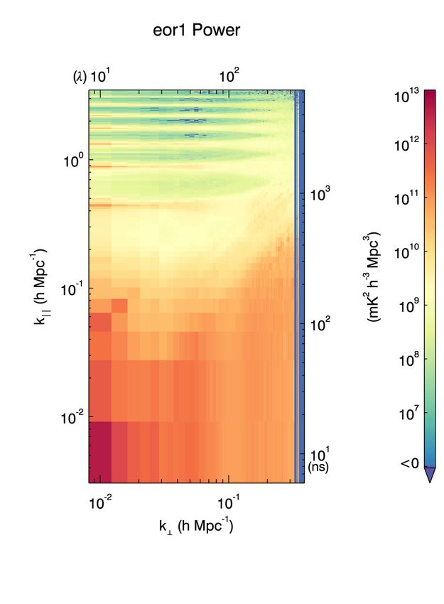
Bispectrum with MWA Phase II                                                                                                    3

Watkinson & Pritchard, 2014). These factors may play a
future important role in discriminating real cosmological
non-Gaussianity from contaminants.
   Despite some work studying the sensitivity of cur-
rent and future experiments for measuring the bispec-
trum (Shimabukuro et al., 2017; Yoshiura et al., 2015),
these have used idealised scenarios that omit any resid-
ual foreground signal and systematics introduced by
the instrument. Bharadwaj & Pandey (2005) discuss
foreground fitting tools using frequency separation to
study the bispectrum over visibility correlations across
frequency, but this method breaks down for large field-
of-view instruments where the interferometric response
affects the foreground smoothness (Morales et al., 2012).
Further, no 21 cm interferometric data has been used
to estimate the bispectrum. In this work, we address
both of these by presenting bispectrum estimators that
can use real datasets, computing the expected impact of
foregrounds measured by the instrument, and applying
the estimators to 21 hours of MWA EoR data.
                                                               Figure 1. Zoomed MWA compact configuration layout showing
2 MWA PHASE II ARRAY                                           the two hexagonal subarrays of 36 tiles each, with redundant
                                                               tile spacings. These short redundant baselines are used in this
The Murchison Widefield Array is a 256-tile low-               work to form equilateral and isosceles triangle bispectra with high
                                                               sensitivity. Some of the longer baseline tiles of the MWA are not
frequency radio interferometer located in the Western          shown.
Australian desert, on the future site of the Square Kilo-
metre Array (SKA) (Tingay et al., 2013; Bowman et al.,
2013). The telescope operates from 80–300 MHz with an-
tennas spread over a 5 km diameter. Its primary science        trum measurement (perfectly-defined triangles formed
areas include exploration of the Epoch of Reionisation,        from discrete baselines). These direct bispectrum results
radio transients, solar and heliospheric studies, study        can be compared to a more general gridded bispectrum,
of pulsars and fast transients, and the production of a        whereby all baselines formed by an irregularly-spaced
full-sky low-frequency extragalactic catalogue. In 2016        array (such as MWA Phase I, or the non-hexagon tiles
it underwent an upgrade from 128 to 256 antenna tiles          of Phase II compact) can be gridded onto the Fourier
(Wayth et al., 2018). At any time, 128 of the tiles can        (uv-) plane, using a gridding kernel that represents the
be connected to the signal processing system. The array        Fourier response function of the telescope (in this case,
operates in a "compact" configuration, utilising redun-        the Fourier Transform of the primary beam response to
dant spacings and short baselines for EoR science, or          the sky). These estimators will both be explored in this
an "extended" configuration, maximising angular res-           work.
olution and instantaneous uv-coverage. The compact
configuration is employed in this work.
   The compact configuration has a maximum baseline            3 POWER SPECTRUM
of 500 metres and is optimised for EoR science. Fig-           We briefly review the power spectrum as the primary
ure 1 shows the tile layout, including the two 36-tile         estimator for studying the EoR with 21 cm observations.
hexagonal subarrays of redundantly-spaced tiles. The           The power spectrum is typically used to describe radio
minimum redundant spacing is 14 m. The primary mo-             interferometer observations from the EoR, and contains
tivations for the hexagons are two-fold: (1) to increase       all of the Gaussian-distributed fluctuation information.
the sensitivity to angular scales of relevance for the EoR,    The power spectrum is the power spectral density of
allowing coherent addition of measurements from redun-         the spatial fluctuations in the 21 cm brightness temper-
dant baselines, and (2) enabling additional methods for        ature field. It is used because it encodes the fluctuation
calibrating the array (redundant calibration, Li et al.        variance (where most of the EoR signal is expected to re-
2018, Joseph et al. 2018). For the bispectrum, there is an     side), and sums signal from across the observing volume
additional advantage of multiple, redundant equilateral        to increase sensitivity. It is defined as:
triangle baselines being formed from the short spacings.
These can be added coherently to study the bispectrum                                                 1
signal on particular scales, and allows for a direct bispec-              P (~k) = δD (~k − ~k 0 )      hV ∗ (~k)V (~k 0 )i,   (1)
                                                                                                     ΩV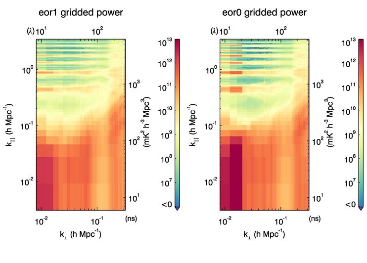
4                                                                                                                       Trott et al.

where V (~k) = V (u, v, η) = FT (V (u, v, ν)) is the mea-             where Nch is the number of spectral channels, ∆ν is the
 sured interferometric visibility (Jansky), Fourier Trans-            spectral resolution, and j and k index frequency and
 formed along frequency (ν) to map frequency to line-                 spatial mode (Hz−1 , or seconds).
 of-sight spatial scales (Jy Hz) at a given point in the                The attenuation of the sky due to the primary beam
 Fourier (uv-) angular plane (u, v); hi encode an ensemble            (and general sky finiteness) alters the complete continu-
 average over different realisations of the Universe, and             ous Fourier Transform to a windowed transform, whereby
 the δD -function ensures that we are expecting to mea-               the primary beam response leaks signal into adjacent
 sure a Gaussian random field where the different modes               Fourier modes, as can be seen using the convolution
 are uncorrelatedi . Further assuming spatial isotropy al-            theorem:
 lows us to average incoherently in spherical shells, where
~k = k. ΩV provides the volume normalisation, where                             V (u, v, η) = Ã(u, v, η) ~ S̃(u, v, η),        (6)
 ΩV = (BW)Ω is the product of the observing bandwidth
 and angular field-of-view. Converting from measured to        where the true sky brightness distribution is convolved
 physical units maps Jy2 Hz2 to mK2 h−6 Mpc6 . After           with the Fourier Transform of the primary beam re-
volume normalisation this becomes, mK2 h−3 Mpc3 .              sponse. This leakage implies that the visibility measured
                                                               by a discrete baseline actually contains signal from a
                                                               region of the Fourier plane, as described by the Fourier
3.1 Power spectra with radio interferometric                   beam kernel, Ã(u, v, η).
      data                                                        In general, to compute the power spectrum from a
The power spectrum can be produced naturally with              large   amount of data, we are motivated by the sig-
interferometric data. Unlike optical telescopes that pro-      nal  weakness  to add the data coherently; i.e., we sum
duce images of the sky, or single-dish radio telescopes        complex visibilities directly that contribute signal to
that acquire a single sky power, a radio interferometer        the same point in the Fourier uv-plane. To do this,
visibility (Jy) directly measures Fourier representations      the measurement from each baseline is convolved with
of the sky brightness distribution at the projected base-      the Fourier beam kernel and ‘gridded’ (added with a
line location (u = ∆x/λ; v = ∆y/λ). In the flat-sky            weight)  onto a common two-dimensional plane. Signal
approximationii :                                              will add coherently, while noise adds as the square-root
                                                               (because the thermal noise is uncorrelated between mea-
              Z
V (u, v, ν) =    A(l, m, ν)S(l, m, ν) exp (−2πi(ul + vm))dldm, surements). The weights for each measurement are also
               Ω
                                                          (4)  gridded with the kernel onto a similar plane. After ad-
where A(l, m, ν) is the instrument primary beam re-            dition of all the data, the signal uv-plane is divided by
sponse to the sky at position (l, m) from the phase            the weights to yield the optimal-weighted average sig-
centre and frequency ν, S(l, m, ν) is the corresponding        nal at each point. The resulting cube resides in (u, v, ν)
sky brightness (Jy/sr, which is proportional to tempera-       space, and can be Fourier Transformed along frequency
ture), and the exponential encodes the Fourier kernel.         to obtain a cube in (u, v, η) space. The power spectrum
The physical correspondence of sky projected on to the         can then be formed by squaring and normalising the
tile locations yields a fixed set of discrete but incom-       cube, and averaging incoherently (in power) in spherical
plete Fourier modes to be measured. This incompleteness        shells:                 X
leads to parts of the Fourier plane where there is no                                      Vi∗ (~k)Vi (~k)Wi (~k)
information. The line-of-sight spatial scales are obtained                  P (|~k|) =
                                                                                       i∈k
                                                                                             X                    ,  (7)
by Fourier Transform of visibilities measured at different                                         Wi (~k)
frequencies, along frequency to map ν to η:                                                  i∈k

                        ∆ν X
                            Nch
                                            2πijk
                                                                     where  W are the weights and |~k| = |(ku , kv , kη )| =
V (η(k)) = FT (V (ν)) =         V (ν) exp −         ,
                                                                      q
                        Nch j=1              Nch                        ku2 + kv2 + kη2 .
                                                               (5)      As an intermediate step, the cylindrically-averaged
                                                                      power spectrum can be formed (e.g., Datta et al., 2010):
    i The   mapping from observed to cosmological dimensions is
given by:                                                                                   X
                                                                                                V ∗ (~k)V (~k)W (~k)
                              2π|u|                                                              i∈k⊥
                     k⊥   =          ,                         (2)
                              DM (z)                                            P (k⊥ , kk ) =          X               ,       (8)
                              2πH0 f21 E(z)
                                                                                                               W (~k)
                     kk   =                 η,                 (3)                                      i∈k⊥
                                c(1 + z)2
where DM is the transverse comoving distance, and f21 is the rest
                                                                                p
frequency of the neutral hydrogen emission.
                                                                      and k⊥ = ku2 + kv2 , kk = kη . This is a useful estimator
   ii This is appropriate for this work where the data used are all   for discriminating contaminating foregrounds (contin-
from zenith-pointed snapshots, where the w-terms are small.           uum sources with power concentrated at small kk ) from
Bispectrum with MWA Phase II 5
21 cm signal. Herein we will refer to this power spec- the sky brightness temperature distribution, measured
trum, and its bispectrum analog, as the ‘gridded power in Jansky.
spectrum’ and ‘gridded bispectrum’, respectively. As discussed earlier, this bispectrum estimator can be
Alternatively, one can take the baselines themselves, unstable, with cosmological simulations showing rapid
and their visibilities measured along frequency, and take fluctuations between positive and negative values as
the Fourier Transform directly along the frequency axis. non-Gaussianity becomes negligible but the amplitude
This ‘delay spectrum’ approach is utilised by some ex- is still large. As such, Watkinson et al. (2018) suggest
periments with short baselines (Parsons et al., 2012; Ali the normalised bispectrum as a more stable statistic:
et al., 2015; Thyagarajan et al., 2015), both to increase √
sensitivity when there are redundant spacings, and to ~ ~ ~ B(k̃1 , k̃2 , k̃3 ) k1 k2 k3
B(k1 , k2 , k3 ) = q , (10)
work as a diagnostic. The frequency and η axes are not P (~k1 )P (~k2 )P (~k3 )
parallel, except at zero-length baseline. Because an in-
terferometer is formed instantaneously from antennas where P (|~k|) is the three-dimensional power spectrum,
with a fixed spatial offset, the baseline length in Fourier which describes the volume-normalised variance on a
space (e.g., u) evolves with frequency as u = ∆xν/c, given spatial scale, and is the Fourier Transform of
and this evolution is therefore increased for larger band- the two-point correlation function (Eggemeier & Smith,
widths and for longer baselines. For the short spacings 2017; Brillinger & Rosenblatt, 1967). This normalisation
of interest to the EoR, the correspondence is good, and isolates the contribution from the non-Gaussianity to
the delay transform can be used to mimic the direct kk the bispectrum, by normalising out the amplitude part
transform of gridded data (see Figure 1 of Morales et al., of the statistic. It is akin to normalising the 3rd central
2012, for a visual explanation). In general, ‘imaging’ ar- moment by σ 3 to calculate the skewness.
rays with many non-redundant spacings are suited to
gridded power spectra, whereas redundant arrays, with
a lesser number of multiply-sampled modes, are suited 4.1 Bispectrum with radio interferometric
to delay power spectra. For the Phase II compact MWA, data
the two hexagonal subarrays have these short-spaced Because the bispectrum is formed from the triple prod-
redundant baselines, and the ‘delay power spectrum’ and uct of a triangle of wavespace measurements, it can be
its bispectrum analog can also be used effectively. In formed directly through the product of three interfero-
general, we would not suggest use of the delay spectrum metric visibilities. In the limit where the array has per-
to undertake EoR science, because of the limitations fect (complete) uv-sampling, individual measurements
discussed, but it is the appropriate analogue for the of signal on triangles of baselines can be multiplied to
direct bispectrum estimator, and is therefore pertinent form the bispectrum estimate. In the more general case,
for the normalised bispectrum analysis. where an interferometer has instantaneously incomplete,
but well-sampled baselines, there are two options for
4 BISPECTRUM extracting the triangles of signal measurements: direct
(via multiplication of measurements from three tiles
The bispectrum is the Fourier Transform of the three- forming a triangle of baselines), or gridded, where each
point correlation function. Akin to the two-point corre- uv-measurement is gridded onto the uv-plane (with its
lation function (the Fourier dual of which is the power corresponding Fourier beam kernel and weights), and the
spectrum), the three-point correlation function measures final bispectra are computed from the fully-integrated
the excess signal over that of a Gaussian random field and gridded data.
distribution measured at three spatial locations, aver- Direct bispectrum estimators can be applied to spe-
aged over the volume. For a field with Fourier Transform cific triangles according to the array layout, but these are
denoted by ∆(~k), the bispectrum is formed over closed usually unique, with irregular configurations (all three
triangles of k vectors in Fourier space: internal angles are distinct), leading to difficult cosmo-
logical interpretation and poor sensitivity. These issues
h∆(~k1 )∆(~k2 )∆(~k3 )i = δD (~k1 , ~k2 , ~k3 )B(k̃1 , k̃2 , k̃3 ). (9) arise for imaging-like arrays with pseudo-random layouts,
but are alleviated for redundant arrays, where regular
Here the δD -function ensures closure in Fourier space. triangles (isosceles and equilateral) exist and are instan-
It has units of mK3 h−6 Mpc6 after volume normalisa- taneously available in many copies in the array. These
tion. The bispectrum is often applied to matter density features make interpretation more straight-forward and
fields, where ∆(~k) is the Fourier Transform of matter increase sensitivity to these bispectrum modes.
overdensity, δ(~x) = ρ(~x)
ρ − 1. In radio interferometric Gridded bispectrum estimators can be applied to any
measurements, the coherence of the wavefront (the vis- array, yield improved sensitivity by coherent gridding
ibilities obtained by cross-correlating voltages from in- of data and may allow for a wider range of triangles to
dividual antennas) represents the Fourier Transform of be probed. Nonetheless, they suffer from the increased6 Trott et al.
difficulty of extracting robust estimates that correctly 5.1 Gridded Estimator noise
account for the correlation of data in uv-space.
The gridded bispectrum estimator is formed from coher-
With the benefit of having a redundant array, we will
ent addition of visibilities over all observations. As such,
apply both sets of estimators to our data.
if a given visibility has thermal noise level σtherm (Jy
Hz)iv , the uncertainty on the bispectrum is:
5 THE GRIDDED ESTIMATOR √ 3
3σ
∆B̂TOT = sX therm , (14)
Each measured visibility encodes information about a
W1 W2 W3
small range of Fourier modes of the sky brightness dis-
Ã
tribution. Although each baseline is usually reported
as a single number representing the antenna separation where the denominator is the sum over the gridding
measured between antenna centres, the baselines actu- kernel of the weights triplets.
ally measure a range of separations when accounting The uncertainty on the normalised bispectrum is then:
for the actual physical sizeiii . This translates to a range s
∆B 2 ∆P12 ∆P22 ∆P32
of Fourier modes being measured by a given baseline, ∆B̂123,TOT = B + 2 + 2 + , (15)
and is equivalent to the statement that a finite primary B 2 4P1 4P2 4P32
beam response to the sky mixes Fourier modes through where the uncertainties can contain both thermal noise
spectral leakage (effectively a taper on the continuous and noise-like uncertainty from residual foregrounds.
Fourier transform). Thus, when measurements from dif- For 300 2-minute observations, and 24 triangles per
ferent baselines are combined coherently (with phase 28 m baseline triad group, the expected thermal noise
information) onto a uv-plane, they can be gridded with level for a complete dataset is:
a kernel that is the Fourier Transform of the primary
∆B = 4.2 × 10¹⁰ mK3 h−6 Mpc6 . (16)
beam response to the sky. Such a gridding kernel cap-
tures the degree of spectral leakage introduced by the The presence of residual foregrounds will be studied in
antenna response, and means that baselines of similar Section 10.2.
length and orientation have some shared information.
The gridding kernel is represented by à in Equation 6.
6 THE DIRECT ESTIMATOR
With a single defined visibility phase centre, all visibility
measurements can be added with this beam kernel onto As an alternate approach to the gridded estimator, vis-
a single plane (for each frequency channel), along with ibilities are Fourier-transformed along the frequency
their associated weights, to form a coherently-averaged direction to compute the delay transform, and closed
estimate for the Fourier representation of the sky bright- bispectrum triangles formed from the closed redundant
ness temperature: triads of antennas. This approach does not use the pri-
X mary beam, and ignores the local spatial correlations
V (ui , vi )Ã(ui , vi )W (ui , vi ) generated by the primary beam spatial taper. It also
i transforms along a dimension that changes angle with
V̂uv = X , (11)
Ã(ui , vi )W (ui , vi ) respect to kk as a function of baseline length, but ap-
i proximates a kk Fourier Transform for small u (small
angle).
where i indexes measurement, and W is the weight The bispectrum for a given observation is the weighted
associated with each. The bispectrum is then estimated average over all triads:
as the sum over the beam-weighted gridded visibilities: X X X
( V1i W1i )( V2i W2i )( V3i W3i )
i i
Xi
X
V̂j1 V̂j2 V̂j3 Wj1 Wj2 Wj3 B̂123 = X X , (17)
j∈Ã
( W1i )( W2i )( W3i )
B̂123 = X , (12) i i i
Wj1 Wj2 Wj3
where i indexes over redundant triangles (triads). The
j
final bispectrum estimate then performs a weighted av-
where erage over observations, such that:
X
W1j = W1 Ã1j , (13) B̂123,j Wj
j
are the beam-gridded measurement weights. B̂123,TOT = X , (18)
Wj
iii Due to the physical size of the collecting antenna element,
j
some parts of the antenna have a smaller effective baseline length
(closer to other antenna), and some have a longer (further from
iv σ = 2kT
therm λ2
Ω √ ∆ν for bandwidth BW, spectral resolu-
BW∆t
the other antenna). tion ∆ν and observation time interval ∆tBispectrum with MWA Phase II 7
where expected to be heavily foreground dominated (i.e., they
X X X correspond to the line-of-sight DC mode, and the large
Wj = ( W1i )( W2i )( W3i ). (19) angular scales of diffuse and point source foreground
i i i emission). We consider them for completeness, but will
show them to be cosmologically irrelevant from an ob-
6.1 Direct Estimator noise servational perspective when computed this way. These
same angularly-equilateral triangle configurations will,
The direct bispectrum estimator is formed from coher- however, be used to form relevant isosceles configura-
ent addition of baseline triplets for a given observation, tions with η1 = η2 and η3 = −2η1 . Given that we aim
which are then averaged with relative weights to the final to sample modes where foregrounds are not dominant
estimate. As such, if a given visibility has thermal noise in our power spectra, these isosceles configurations form
level σtherm (Jy Hz), the uncertainty on the bispectrum ‘stretched’ (also referred to ‘flattened’ in Watkinson et al.,
is: √ 3 2018) configurations (kk >> k⊥ ). Figure 2 shows how
3σtherm
∆B̂TOT = sX . (20) the stretched isosceles configurations are extracted from
Wj the data with a redundant baseline triad. Figure 3 then
j shows schematically the approximate vectors for two of
the four isosceles configurations considered here.
The uncertainty on the normalised bispectrum is then
given by the same expression as for the Gridded Esti-
mator (Equation 15). 8 OBSERVATIONS
For 300 observations, and 24 triangles per 28 m base- The direct and gridded estimators are applied to 21.0
line triad group, the expected noise level is: hours of Phase II high-band zenith-pointed data, com-
prising 10.7 hours (320 observations) on the EoR0 field
∆B = 7.1 × 10¹¹ mK3 h−6 Mpc6 . (21)
(RA= 0 h, Dec.= −27 deg.) and 10.3 hours (309 observa-
tions) on the EoR1 field (RA= 4 h, Dec.= −30 deg.). We
7 TRIANGLES CONSIDERED FOR observe 30.72 MHz in 384 contiguous 80 kHz channels,
ESTIMATION with a base frequency of 167.035 MHz. Approximately
15% of the observations were obtained from drift-scan
Unlike bispectrum estimates that can be obtained from
data, where the telescope remains pointed at zenith for
Phase I data, where the array is in an imaging config-
many hours and the sky drifts through. For consistency
uration with no redundant triangles, we aim to take
with the drift-n-shift data, we chose drift scan data ob-
advantage of the 72 redundant tiles in the hexagonal
served with the field phase centres within 3 degrees of
sub-arrays, afforded by the Phase II layout. This allows
zenith. The data were observed over five weeks from
for both direct and gridded bispectrum estimators to
2016 October 15 to November 28, and one week in 2017
be applied to matched observations with matched data
July. Because the delay spectrum is used as part of the
calibration.
power spectrum estimator for the direct bispectrum,
The most numerous (highest sensitivity) groups of
each observation was individually inspected for poor
redundant triangles are the angularly-equilateral config-
calibration or data quality, and bad observations excised
urations of the 14 m and 28 m baselines (48 and 24 sets,
from the dataset. The excised observations comprised
respectively). For these triangles, the equilateral config-
∼5 percent of the dataset, and primarily were due to
urations exist only for the η = 0 (kk = 0) line-of-sight
poor calibration solutions over sets of data contiguous
mode. Other configurations of these closed angular trian-
in time due to poor instrument conditions (e.g., many
gles are isosceles or irregular triangles, depending on the
flagged tiles or spectral channels).
η values chosen, however the closed triangle requirement
of the bispectrum demands that: The 2-minute observations were each calibrated
through the MWA Real Time System (RTS; Mitchell et
η1 + η2 + η3 = 0, (22) al. 2008), as is routinely performed for MWA EoR data,
and one thousand of the brightest (apparent) sources
in addition to the angular components of the vectors peeled from the dataset (Jacobs et al., 2016). These
summing to zero (as is enforced by choosing the closed 629 calibrated and peeled observations were used for
triangle baselines). bispectrum estimation.
For comparison with theoretical predictions, we will
focus on equilateral and isosceles triangles. The 14 m
9 RESULTS
and 28 m baselines are very short, corresponding to
cosmological scales of k⊥ ' 0.01hMpc−1 at z = 9. Thus, We begin by reporting the bispectrum estimates for the
although the equilateral configuration is cosmologically two methods and fields, and then report the normalised
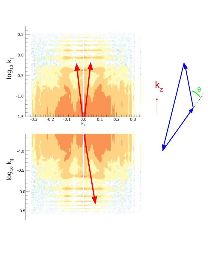
relevant and the easiest to interpret, these modes are bispectra, which incorporate the power spectrum es-8 Trott et al. Figure 2. Schematic of how a stretched isosceles triangle configuration is extracted from redundant angularly-equilateral triangle baselines of the MWA Phase II hexagons. timates. Table 1 shows the bispectrum estimates and beams, and Fourier Transform along frequency, yielding their one sigma uncertainties (thermal noise) for the different results for longer baselines. The signature of direct and gridded estimators, both observing fields and Galactic emission from close to the horizon is evident for different triangle configurations. Bold-faced results in the EoR0 power spectra, while it is less structured in indicate bispectrum estimates that are consistent with EoR1, where the Galactic Centre has set. Most notably, thermal noise. These tend to be those that are extremely the delay spectra show large foreground leakage into the stretched isosceles configurations (cos θ ∼ 1), with es- EoR window (kk < 0.4), yielding large power spectrum timates that sit well outside the primary foreground denominator values for the normalised bispectrum. contamination parts of parameter space. Conversely, the Using these data, Table 2 describes the normalised bis- equilateral triangle configurations that use the kk = 0 pectrum. Bold-faced results are broadly consistent with mode exclusively show extremely large detections. There thermal noise (< 5σ), again reflecting the modes that is no suggestion that these are 21 cm cosmological bis- are least affected by foregrounds. The difference between pectrum detections, but rather are foreground contam- the dimensional and reduced bispectrum results is due inants. This will be explored more fully in Section 10. to the different power spectral estimators. Also notable Note also that the thermal noise levels reported here are is the difference in amplitude of the gridded and direct a factor of a few larger than the theoretical expectation normalised bispectrum estimates. Due to the division derived in Sections 5–6. This is due to the fraction of by the power spectrum, the normalised bispectrum is data with weights that are less than unity, indicating heavily-dependent on the details of the power spectrum flagged baselines and spectral channels. estimates, which fluctuate substantially in foreground- Also listed in Table 1 is the expected bispectrum affected regions. The delay-space power spectra show values from simulations that assume either bright or faint increased foreground power in the EoR window, and this galaxies drive reionization (Greig & Mesinger, 2017). The is reflected in a larger power spectrum estimate, and largest amplitudes are for the smallest k-modes, which therefore a lower normalised bispectrum. This reliance also tend to be more foreground dominated. highlights the complexity for interpreting the normalised The normalised bispectrum, B, is normalised by the bispectrum with foreground-affected data. power spectra at each of the k modes forming the trian- gles. Figure 4 shows the power spectra for the EoR1 and 10 BISPECTRUM SIGNATURE OF EoR0 fields for the full datasets as used in the gridded es- FOREGROUNDS timator. These have been processed through the CHIPS power spectrum estimator (Trott et al., 2016). Figures Estimates of bispectrum sensitivity for operational and 5 and 6 show the corresponding delay spectra, as used future 21 cm experiments are incomplete without a treat- in the direct bispectrum. There are small differences ment of foregrounds. Despite the expectation that point between the two power spectrum estimators, as is ex- source, continuum foregrounds only impact a region of pected given that delay spectra do not grid with primary the three dimensional EoR parameter space (kx , ky , kk ),
Bispectrum with MWA Phase II                                                                                                    9

Figure 3. Schematic of how isosceles triangle vectors are extracted, overlaid on a power spectrum. We aim to choose triangles with
vectors that reside in noise-like regions of the delay spectrum.
10                                                                                                               Trott et al.

               Triangles                  Direct                  Gridded               Type         Faint Galaxy
                EoR0                (×1012 mK3 Mpc6 )        (×1012 mK3 Mpc6 )          14m          (mK3 Mpc6 )
         k1 = k2 = k3 = 0.007          1.3e9 ± 7.8              4.3e8 ± 0.2          Equilateral
        k1 = 0.2, k2 = k3 = 0.1       −1071.2 ± 7.8             −1.6e4 ± 0.2          Isosceles        4.4 × 10⁹
        k1 = 0.4, k2 = k3 = 0.2        −7571 ± 7.8              8.9e4 ± 0.2           Isosceles       −2.7 × 10⁷
        k1 = 0.6, k2 = k3 = 0.3        27250 ± 7.8              −1078 ± 0.2           Isosceles       −3.6 × 10⁶
        k1 = 1.0, k2 = k3 = 0.5         47.0 ± 7.8               22.0 ± 0.2           Isosceles        5.8 × 10⁴
                EoR0                                                                    28m
         k1 = k2 = k3 = 0.014         −1.3e7 ± 22.2             6.9e8 ± 0.3          Equilateral
        k1 = 0.2, k2 = k3 = 0.1        120.8 ± 22.2              9582 ± 0.3           Isosceles
        k1 = 0.4, k2 = k3 = 0.2       −2010 ± 22.2              −84.0 ± 0.3           Isosceles
        k1 = 0.6, k2 = k3 = 0.3        943.2 ± 22.2              65.1 ± 0.3           Isosceles
        k1 = 1.0, k2 = k3 = 0.5        13.7 ± 22.2               88.2 ± 0.3           Isosceles
                EoR1                (×1012 mK3 Mpc6 )        (×1012 mK3 Mpc6 )          14m          Bright Galaxy
         k1 = k2 = k3 = 0.007          −9.9e6 ± 2.3             2.0e10 ± 0.3         Equilateral
        k1 = 0.2, k2 = k3 = 0.1        −21.5 ± 2.3              1.9e4 ± 0.3           Isosceles        4.4 × 10⁹
        k1 = 0.4, k2 = k3 = 0.2         978.9 ± 2.3             −4.0e8 ± 0.3          Isosceles       −2.9 × 10⁷
        k1 = 0.6, k2 = k3 = 0.3        1546.4 ± 2.3             −25.4 ± 0.3           Isosceles       −8.4 × 10⁵
        k1 = 1.0, k2 = k3 = 0.5        −2.0 ± 2.3                0.4 ± 0.3            Isosceles        1.5 × 10⁵
                EoR1                                                                    28m
         k1 = k2 = k3 = 0.014            3.6e5 ± 6.7            −1.2e8 ± 0.5         Equilateral
        k1 = 0.2, k2 = k3 = 0.1           2.7 ± 6.7             −1530 ± 0.5           Isosceles
        k1 = 0.4, k2 = k3 = 0.2           1.7 ± 6.7             203.3 ± 0.5           Isosceles
        k1 = 0.6, k2 = k3 = 0.3         −229.4 ± 6.7            −12.5 ± 0.5           Isosceles
        k1 = 1.0, k2 = k3 = 0.5          37.1 ± 6.7             474.3 ± 0.5           Isosceles
Table 1 Bispectrum estimates and one sigma uncertainties for the direct and gridded bispectra for each observing field and
triangle type. Bold-faced values indicate bispectrum estimates that are consistent with thermal noise. The right-hand column
lists expected bispectrum values from simulation for faint and bright galaxies driving reionisation. k modes are comoving and
measured in h Mpc−1 .
Bispectrum with MWA Phase II 11 Figure 4. Gridded power spectra for the 21 hours of observations on two fields used in this work, as processed through the CHIPS estimator (Trott et al., 2016).
12                                                                                                            Trott et al.

                          Triangles                  Direct              Gridded             Type
                           EoR0                                                              14m
                    k1 = k2 = k3 = 0.007        0.166 ± 2.5e − 7      10.4 ± 4.1e − 8     Equilateral
                   k1 = 0.2, k2 = k3 = 0.1      −0.266 ± 0.0004         921.2 ± 0.3        Isosceles
                   k1 = 0.4, k2 = k3 = 0.2       2.84 ± 0.0044        −1766.2 ± 0.6        Isosceles
                   k1 = 0.6, k2 = k3 = 0.3       −4.87 ± 0.063         −427.8 ± 5.8        Isosceles
                   k1 = 1.0, k2 = k3 = 0.5         3.45 ± 0.60        129.4 ± 108.9        Isosceles
                           EoR0                                                              28m
                    k1 = k2 = k3 = 0.014       −0.019 ± 1.4e − 7     −29.3 ± 8.1e − 6     Equilateral
                   k1 = 0.2, k2 = k3 = 0.1      −0.14 ± 0.002         −594.5 ± 4.0         Isosceles
                   k1 = 0.4, k2 = k3 = 0.2      0.360 ± 0.009          948.9 ± 7.2         Isosceles
                   k1 = 0.6, k2 = k3 = 0.3       0.98 ± 0.18          −793.1 ± 37.6        Isosceles
                   k1 = 1.0, k2 = k3 = 0.5       1.08 ± 1.78           19450 ± 752         Isosceles
                           EoR1                                                              14m
                    k1 = k2 = k3 = 0.007       −0.004 ± 1.2e − 8      0.61 ± 3.2e − 9     Equilateral
                   k1 = 0.2, k2 = k3 = 0.1      0.044 ± 0.0001        −666.5 ± 0.03        Isosceles
                   k1 = 0.4, k2 = k3 = 0.2       0.19 ± 0.0004         3157.0 ± 0.82       Isosceles
                   k1 = 0.6, k2 = k3 = 0.3      −0.064 ± 0.007        −1861.9 ± 0.54       Isosceles
                   k1 = 1.0, k2 = k3 = 0.5      −0.12 ± 0.13           5907.5 ± 56.1       Isosceles
                           EoR1                                                              28m
                    k1 = k2 = k3 = 0.014       0.0006 ± 7.0e − 9      17.1 ± 8.4e − 7     Equilateral
                   k1 = 0.2, k2 = k3 = 0.1     0.0001 ± 0.0005          927.7 ± 0.43       Isosceles
                   k1 = 0.4, k2 = k3 = 0.2      −0.082 ± 0.002        −245.3 ± 0.15        Isosceles
                   k1 = 0.6, k2 = k3 = 0.3      0.012 ± 0.030          5881.8 ± 10.4       Isosceles
                   k1 = 1.0, k2 = k3 = 0.5         6.2 ± 1.2           4257.6 ± 15.6       Isosceles
Table 2 Normalised bispectrum estimates, B, and one sigma uncertainties for the direct and gridded bispectra for each
observing field and triangle type. Bold-faced values indicate bispectrum estimates that are consistent with thermal noise.
Bispectrum with MWA Phase II 13
Figure 6. Delay transform power spectra for the EoR0 field for
the data used in this analysis.
in reality the details of the instruments, complexity of
extragalactic and Galactic emission, limited bandwidth
and calibration errors leave residual contaminating sig-
nal throughout the full parameter space. Although these
methods perform very well to remove such signal, the
extreme dynamic range demanded by this experiment
translate to bias that exceeds the expected cosmological
signal strength. The results presented here are clearly
foreground-dominated, particularly for the equilateral
Figure 5. Delay transform power spectra for the EoR1 field for triangle configuration.
the data used in this analysis. Note the large leakage into the
EoR window, which yields large denominators for the normalised
As such, the bispectrum signature of foregrounds can
bispectrum. be computed for a simple point source foreground model.
We first consider the expected foreground bispectrum,
which quantifies the bias in the measurement, and then
turn to the variance of the foreground bispectrum, which
quantifies the additional noise term.
We employ a model where the sky is populated with
a random distribution of unresolved extragalactic point
sources that follow a low-frequency number counts dis-
tribution (Intema et al., 2011; Franzen et al., 2016):
dN
= αS β Jy−1 sr−1 , (23)
dS
where α ' 3900 and β = −1.59 for sources with flux
density at 150 MHz of less than 1 Jansky. We assume
there is no source clustering and spectral dependence,14 Trott et al.
yielding a Poisson-distributed number of sources in each sources are only correlated locally (δD (l1 + l2 + l3 = 0)),
differential sky area. its expected value with respect to foregrounds is:
The clustering of point sources in the power spectrum Z
3 3 2 2 2
has been studied by Murray et al. (2017). They find hV1 V2 V3 i = dldmhS (l, m)iA (l, m) exp −2π Σ T
that source clustering will be unimportant for the MWA (29)
(unless the clustering is extreme, which is not measured), where,
but may be important for the SKA, which can clean 2
x1 l y1 m
to deeper source levels. Nonetheless, the structure due T2 = + − η1
c c
to clustered point source foregrounds only changes the 2 2
x2 l y2 m x3 l y3 m
amplitude of the foreground structure in the EoR wedge + + − η2 + + − η3 (30)
.
c c c c
as a function of angular scale (k⊥ ). Because the line-of-
sight spectral component is unaffected, the signature of Here, the source counts have been separated from the
clustered foregrounds in the EoR Window is mostly un- spatial integral. This is a general expression for a triplet
changed. These more realistic point source foregrounds of baselines. We can now simplify this for triangles,
will be considered in the simulations of Watkinson & particularly those with isosceles configurations (where
Trott (2019) and here we retain the analytic signature the equilateral is a single case of an isosceles).
of the Poisson foregrounds. Closed triangles follow the relations:
We further assume that the primary beam can be x1 + x2 = −x3 (31)
approximated by a frequency-dependent Gaussian:
y1 + y2 = −y3 (32)
(l2 + m2 )ν02 Aeff
η1 + η2 = −η3 , (33)
A(l, m, ν0 ) = exp − , (24)
2c2 2
and we define, without loss of generality, the following
where Aeff is the tile effective area, and encodes the relations for the isosceles configurations considered in
conversion from an Airy disk to a Gaussian. this work:
The visibility is given by Equation 4 for frequency ν.
To compute the line-of-sight component to the visibility, x1 = −2x2
we Fourier Transform over frequency channels, after x2 = x3
employing a frequency taper (window function) to reduce y1 = 0
spectral leakage from the finite bandwidth:
y2 = −y3
√
Z
V (u, v, η) = dldmS(l, m, ν0 )A(l, m, ν0 ) y2 = x1 cos π/6 = 2x2 cos π/6 = 3x2
Z 2η2 = 2η3 = −η1 . (34)
ν(xl + ym)
× dνΥ(ν) exp −2πi exp (−2πiνη)
c Making these substitutions in Equation 29, completing
the squares and collecting terms, we find:
Z
= dldmS(l, m, ν0 )A(l, m, ν0 ) Z
Z hV1 V2 V3 i = dldmhS 3 (l, m)iA3 (l)
× dνΥ(ν) exp (−2πiν(xl/c + ym/c + η)) (25)
× exp −12π 2 Σ2 x22 /c2 (l2 + m2 ) + η22 .
Z (35)
= dldmS(l, m)A(l, m) The source count expectation value uses the source num-
ber counts distribution and the fact that the number
× Υ̃(xl/c + ym/c + η) JyHz, (26)
of sources at any sky location is Poisson-distributed to
whee Υ(ν) is the spectral taper, and we have per- find:
formed the Fourier Transform over frequency. For ana- 3
Z
dN
lytic tractability, in this work we use a Gaussian taper, hS (l, m)i = S 3 (ν0 )
S dS
with a characteristic width, Σ 'BW/7, such that the α
edges of the band are consistent with zero and it is = S 4+β
Jy3 sr−1 (36)
4 + β max
well-matched to a Blackman-Harris taper:
Incorporating the primary beam from Equation 24,
ν2 moving to polar coordinates, and performing the inte-
Υ(ν) = exp − 2 , (27)
2Σ gral over (l, m), we find for the expected foreground
with corresponding Fourier Transform, bispectrum bias:
√ α
Υ̃(η) = 2πΣ2 exp −2π 2 Σ2 η 2 Hz. (28) hV1 V2 V3 i = (2πΣ2 )1.5 S 4+β
4 + β max
π 2 BW2 η22
The bispectrum is formed from the triple product π
of visibilities. Accounting for the fact that the point × exp − Jy3 Hz3 (37)
θ 25Bispectrum with MWA Phase II 15
Interestingly, the expected foreground bispectrum
signal is positive, due to its constituent astrophysical
sources being associated with overdensities. Conversely,
the stretched isosceles 21-cm bispectrum from the cos-
mological signal will be negative on many scales during
reionisation (Majumdar et al., 2018).
10.1 Normalised foreground bispectrum
The normalised bispectrum also contains the expected
power spectrum values for a foreground model. In line
with the methodology developed in the previous section,
we can write the expected power spectrum at (u, v, η)
as:
P (u, v, η) = hV ∗ (u, v, η)V (u, v, η)i
Figure 7. Point source-foreground dimensional bispectrum sig- α
nature of isosceles triangle vectors in k⊥ − kk -space (note the = (2πΣ2 ) S 3+β
stretched logarithmic colour bar). In this model, the expected 3 + β max
foreground signal has fallen to below the expected cosmological b + 2a b − 2a
signal value by kk ≥ 0.12. × erf √ − erf √
2a 2a
2
r
π b
× exp −4π 2 Σ2 η 2 exp , (41)
4a 4a
where,
3Aeff ν02 π 2 BW2 u22 where
θ= + , (38)
c2 25ν02
2πc2 4Σ2 |x|2
and BW is the experiment bandwidth. This factor com- a = + (42)
ν02 Aeff /2 c2
bines the primary beam (spatial taper) and spectral 2
taper components into a single factor. 8Σ |x|η
b = , (43)
The equilateral configuration can be derived from c
this expression with η2 = 0. For the 28 m baselines, a
encode the spatial and spectral tapers, and |x|2 = x2 +y 2
maximum source flux density of 1 Jy and Aeff = 21 m2 ,
(without loss of generality). This expression is derived
and performing the cosmological conversions, we expect
from the Fourier Transform over Gaussians, and then
a bispectrum estimate of:
the integral over dldmv .
B(x = 28) ' 8.6 × 10¹⁹ mK3 h−6 Mpc6 , (39) When η = 0 and for the 28 m baseline triangles, the
expected bispectrum normalisation is:
which is comparable to the estimates found in Sec- p
tion 9. For 14 m baselines, B(x = 14) ' 1.0 × P (u, v, η)3 /V = 2.8 × 10²¹ mK3 h−6 Mpc6 . (44)
1020 mK3 h−6 Mpc6 . p
The isosceles configurations incorporate the η term. For the 14 m triangles, we find, P (u, v, η)3 /V = 3.3 ×
For kk > 0.1, this term decays to below the noise, 1021 mK3 h−6 Mpc6 . When compared with the expected
which is consistent with that observed in the data. The bispectrum value, we find that (28 m):
signature of this isosceles foreground dimensional bis-
pectrum in k⊥ -kk space is shown in Figure 7. For the hBi = 1.7, (45)
k1 = 0.1h Mpc−1 stretched configuration, we expect for
28 m (14 m): and hBi = 0.6 for the 14 m baselines, which exceed
the equilateral triangle configuration estimates from
B ' 1.7 × 10¹² (1.0 × 10¹² )mK3 h−6 Mpc6 . (40) the MWA data. As with the bispectrum estimate, the
isosceles configurations have expected power values
The squeezed configurations of large k⊥ combined with that fall rapidly with η, and are less comparable to
small kk might be interesting for future studies, depend- the data in these idealised scenarios. However, for the
ing on the expected cosmological signal on these scales.
v This can also be derived as a covariance between u modes
Given that the power spectrum is expected to be small
and η modes, which encodes the spectral leakage that stems from
on these combination of line-of-sight and angular scales, the spatial and spectral tapers. This covariance is that used to
most EoR experiments are not designed for high sensi- understand power spectrum uncertainties in EoR work, where
tivity here (k⊥ = 0.1 corresponds to 200 m baselines). correlations between k-cells must be correctly treated.16 Trott et al.
10.2 Foreground bispectrum error
We now turn our attention to consideration of the signal
2
variance due to residual foregrounds, hBFG i, such that
(cf Equation 14):
3σ 6 2
∆B 2 = Xtherm + hBFG i, (47)
Wj
j
and
2
hBFG i = hV1∗ V2∗ V3∗ V1 V2 V3 i. (48)
This reduces to a relatively simple expression for the sim-
ple point source case, due to the cancelling of complex
components (this is not generally true for the covari-
ance). Using the same formalism as earlier, and again
considering the Poisson-distributed nature of the flux
density of the sources, we find:
Figure 8. Point source- normalised foreground bispectrum sig-
nature of isosceles triangle vectors in k⊥ − kk -space (note the Z Z
2 6 dN
stretched logarithmic colour bar). In this model, the expected hBFG i = S dS A6 (l, m)dldm (49)
foreground signal has fallen to below the expected cosmological dS
Z
signal value by kk ≥ 0.12.
× ~ (−2πi(η1 ∆ν12 +η2 ∆ν34 +η3 ∆ν56 ) d~ν
Υe
S 7+β c2 2
2 2 2 2 2
= α max 12π 2 e−4π Σ (η1 +η2 +η3 ) ,
k1 = 0.1h Mpc−1 stretched configuration, we expect for 7+β ν0 Aeff
7+β
c2 2
28 m (14 m): S 2 2 2
= α max 12π 2 e−6π Σ η1 ,
7+β ν0 Aeff
hBi = 4.0 (240, 000). (46)
where Υ ~ ≡ Υ(ν1 )Υ(ν2 )Υ(ν3 )Υ(ν4 )Υ(ν5 )Υ(ν6 ). This ex-
These values are ratios of very small numbers, and there- pression is flat in angular modes, and decays rapidly in
fore are highly dependent on numerical details and are line-of-sight modes.
not representative. However, they may lend support to Comparing this with the expected value of the fore-
the idea that the normalised bispectrum is difficult to ground bispectrum, Equation 37, we can form the fore-
interpret because it relies on foreground details in both ground bispectrum signal-to-error ratio; Figure 9. The
the bispectrum and power spectrum. signal bias exceeds the uncertainty for small scales,
Alternatively, the combination of power spectrum, di- but on the larger scales of interest for EoR, the uncer-
mensional bispectrum and normalised bispectrum may tainty dominates. Nonetheless, there is no line-of-sight
help to shed additional light on whether data are re- dependence, demonstrating that the foreground bias
ally foreground free. Given the different behaviour of and uncertainty both drop rapidly and are negligible
foregrounds in these statistics, this information may be for kk > 0.12hMpc−1 , implying that for larger kk scales,
used to discriminate cosmological information from fore- point source foregrounds are not significant in the signal
grounds, or to help to design some iterative foreground or noise budget.
cleaning algorithm, taking into consideration their be- One can also now compare the foreground uncertainty
haviour in cosmological simulations. In this scenario, the to the expected thermal noise level. For the EoR1 field
normalised bispectrum may provide useful information. data, the measured uncertainty for the direct bispec-
Figure 8 displays the normalised foreground bispec- trum estimator was 6.7 × 10¹² mK3 Mpc6 . Figure 10
trum for isosceles configurations in k⊥ −kk space. For the shows this level (green line) compared with the fore-
point source foregrounds, the power spectrum denom- ground bispectrum error (red line) as a function of
inator dominates over the expected bispectrum signal, line-of-sight scale. (The gridded estimator has slightly
yielding values < 10−3 across all of parameter space. lower noise level, but the distinction is not significant
This presents an interesting divergence from the usual when compared to the large gradient of the foreground
expectation of foreground bias in the power spectrum, contribution.) As with the foreground bias, the error
where foregrounds add overall signal. In this case, a large induced by residual foregrounds drops steeply beyond
measurement that exceeds the thermal noise is consis- kk = 0.12hMpc−1 , and falls below the thermal noise
tent with a cosmological origin, and not with residual (even in this case with a small dataset for the EoR1
foregrounds. field).Bispectrum with MWA Phase II 17
As a final step to assessing the advantages of the
bispectrum compared with the power spectrum to de-
tect the cosmological signal, we divide the expected
21 cm bispectrum values for the faint and bright galax-
ies, presented in Table 1 by the foreground error for
these modes, and compare with that for the power spec-
trum. The power spectrum values for faint and bright
galaxies are taken from the same underlying dataset
generated by 21cmFAST (Mesinger et al., 2011). For all
but the k1 = 0.1hMpc−1 mode, the foreground uncer-
tainty is negligible, and the ratio is uninteresting. For
k1 = 0.1hMpc−1 , k2 = k3 = 0.2hMpc−1 :
P21 = 1.3 × 10⁴ mK 2 M pc3
∆PF G = 0.2 × 10⁻¹ mK 2 M pc3
B21 = 4.4 × 10⁹ mK 3 M pc6
∆BF G = 4.6 × 10¹⁰ mK 3 M pc6 , (50)
yielding better performance for the power spectrum,
within the foreground dominated region.
However, outside of the foreground ‘wedge’, which
exists in both power spectrum and bispectrum space,
Figure 9. Ratio of point source foreground bispectrum bias to
uncertainty, for isosceles triangle vectors in k⊥ − kk -space (note the data uncertainty is limited by the thermal noise, and
linear plot). The bias exceeds the uncertainty at large angular here the bispectrum achieves higher signal-to-noise ratio
modes, but rapidly falls below for larger k⊥ , with no dependence for a set observation time:
on line-of-sight scale.
P21 = 1.3 × 10⁴ mK 2 M pc3
∆Ptherm = 5.7 × 10⁶ mK 2 M pc3
B21 = 4.4 × 10⁹ mK 3 M pc6
∆Btherm = 5.3 × 10¹¹ mK 3 M pc6 . (51)
Taking the ratios we find,
P21 /∆Ptherm = 0.002
B21 /∆Btherm = 0.008.
Accounting for the fact that the gridded bispectrum av-
erages down with t1.5 while the gridded power spectrum
averages with t, the observing time multiple (above 10
hours) for a detection (SNR=1) is
tP = 500 ×
tB = 25 × .
Therefore, the bispectrum detection can theoretically be
achieved in a fraction of the time of the power spectrum
detection, for thermal noise-limited modes close to the
EoR wedge. A SNR=1 detection level could potentially
be reached in 250 hours, for this wave mode. This con-
clusion is relevant for the MWA, where the excellent
instantaneous uv-coverage allows for rapid observation
of triangle configurations. (We note that the power spec-
Figure 10. Errors for point source-normalised foreground bispec-
trum (red) and thermal noise (green), for isosceles triangle vectors
trum SNR shown here is not inconsistent with previous
in k⊥ − kk -space and 300 observations used in this work for the expectations for the performance of the MWA, because
EoR1 field. it applies only to this single mode; Beardsley et al., 2016;
Wayth et al., 2018). Future work presented in Watkinson
& Trott (2019) will explore a more full range of triangle
configurations and foreground bias and error.You can also read