Bridge Composite and Real: Towards End-to-end Deep Image Matting - arXiv
←
→
Page content transcription
If your browser does not render page correctly, please read the page content below
Noname manuscript No.
                                         (will be inserted by the editor)

                                         Bridge Composite and Real: Towards End-to-end Deep
                                         Image Matting
                                         Jizhizi Li1 , Jing Zhang1 , Stephen J. Maybank2 , Dacheng Tao1 ,
arXiv:2010.16188v2 [cs.CV] 11 Jul 2021

                                         Received: date / Accepted: date

                                         Abstract Extracting accurate foregrounds from natu-         images. Comprehensive empirical studies have demon-
                                         ral images benefits many downstream applications such       strated that GFM outperforms state-of-the-art meth-
                                         as film production and augmented reality. However, the      ods and effectively reduces the generalization error. The
                                         furry characteristics and various appearance of the fore-   code and the dataset will be released.
                                         grounds, e.g., animal and portrait, challenge existing
                                         matting methods, which usually require extra user in-
                                         puts such as trimap or scribbles. To resolve these prob-    1 Introduction
                                         lems, we study the distinct roles of semantics and de-
                                         tails for image matting and decompose the task into         Image matting refers to extracting the foreground alpha
                                         two parallel sub-tasks: high-level semantic segmenta-       matte from an input image, requiring both hard labels
                                         tion and low-level details matting. Specifically, we pro-   for the explicit foreground or background and soft labels
                                         pose a novel Glance and Focus Matting network (GFM),        for the transition areas, which plays an important role
                                         which employs a shared encoder and two separate de-         in many applications, e.g., virtual reality, augmented
                                         coders to learn both tasks in a collaborative manner        reality, entertainment, etc. Typical foregrounds in the
                                         for end-to-end natural image matting. Besides, due to       task of image matting have furry details and diverse ap-
                                         the limitation of available natural images in the mat-      pearance, e.g., animal and portrait, which lay a great
                                         ting task, previous methods typically adopt compos-         burden on image matting methods. How to recognize
                                         ite images for training and evaluation, which result in     the semantic foreground or background as well as ex-
                                         limited generalization ability on real-world images. In     tracting the fine detail for trimap-free natural image
                                         this paper, we investigate the domain gap issue be-         matting remains challenging in the image matting com-
                                         tween composite images and real-world images system-        munity.
                                         atically by conducting comprehensive analyses of vari-          For image matting, an image I is assumed to be a
                                         ous discrepancies between foreground and background         linear combination of foreground F and background B
                                         images. We find that a carefully designed composition       via a soft alpha matte α ∈ [0, 1], i.e.,
                                         route RSSN that aims to reduce the discrepancies can
                                         lead to a better model with remarkable generalization       Ii = αi Fi + (1 − αi ) Bi ,                           (1)
                                         ability. Furthermore, we provide a benchmark contain-
                                         ing 2,000 high-resolution real-world animal images and      where i denotes the pixel index. It is a typical ill-posed
                                         10,000 portrait images along with their manually la-        problem to estimate F, B, and α given I from Eq. (1)
                                         beled alpha mattes to serve as a test bed for evaluat-      due to the under-determined nature. To relieve the bur-
                                         ing matting model’s generalization ability on real-world    den, previous matting methods adopt extra user input
                                                                                                     such as trimap (Xu et al., 2017) and scribbles (Levin
                                              Jing Zhang (jing.zhang1@sydney.edu.au)
                                                                                                     et al., 2007) as priors to decrease the degree of unknown.
                                              Dacheng Tao (dacheng.tao@sydney.edu.au)                Based on sampling neighboring known pixels (Wang
                                         1   The University of Sydney, Sydney, Australia             and Cohen, 2007; Ruzon and Tomasi, 2000; Wang and
                                         2   Birkbeck College, London, U.K.                          Cohen, 2005) or defining an affinity matrix (Zheng et al.,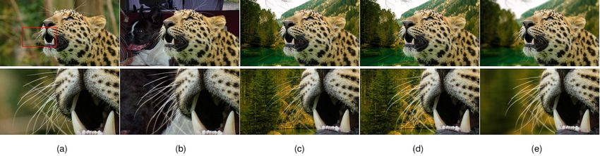
2                                                             Jizhizi Li1 , Jing Zhang1 , Stephen J. Maybank2 , Dacheng Tao1 ,

2008), the known alpha values (i.e., foreground or back-         ting and explore the idea of decomposing the task into
ground) are propagated to the unknown pixels. Usually,           two parallel sub-tasks, semantic segmentation and de-
some edge-aware smoothness constraints are used to               tails matting. Specifically, we propose a novel end-to-
make the problem tractable (Levin et al., 2007). How-            end matting model named Glance and Focus Matting
ever, either the sampling or calculating affinity matrix         network (GFM). It consists of a shared encoder and
is based on low-level color or structural features, which        two separate decoders to learn both tasks in a col-
is not so discriminative at indistinct transition areas          laborative manner for natural image matting, which
or fine edges. Consequently, their performance is sensi-         is trained end-to-end in a single stage. Moreover, we
tive to the size of unknown areas and may suffer from            also explore different data representation formats in
fuzzy boundaries and color blending. To address this             the global decoder and gain useful empirical insights
issue, deep convolutional neural network (CNN)-based             into the semantic-transition representation. As shown
matting methods have been proposed to leverage its               in Figure 1(a)(iii), compared with previous methods,
strong representative ability and the learned discrim-           GFM is a unified model that models both sub-tasks
inative features (Xu et al., 2017; Chen et al., 2018;            explicitly and collaboratively in a single network.
Zhang et al., 2019; Qiao et al., 2020; Liu et al., 2020; Yu          Another challenge for image matting is the limi-
et al., 2021). Although CNN-based methods can achieve            tation of available matting dataset. As shown in Fig-
good matting results, the prerequisite trimap or scrib-          ure 1(b) ORI-Track, due to the laborious and costly
bles make them unlikely to be used in automatic appli-           labeling process, existing public matting datasets only
cations such as the augmented reality of live streaming          have tens or hundreds of high-quality annotations (Rhe-
and film production.                                             mann et al., 2009; Shen et al., 2016; Xu et al., 2017;
    To address this issue, end-to-end matting methods            Zhang et al., 2019; Qiao et al., 2020). They either only
have been proposed (Chen et al., 2018; Zhang et al.,             provide foregrounds and alpha mattes (Xu et al., 2017;
2019; Shen et al., 2016; Qiao et al., 2020; Liu et al.,          Qiao et al., 2020) as in (i) of Figure 1(b) ORI-Track,
2020) in recent years. Most of them can be catego-               or provide fix-size and low-resolution (800 × 600) por-
rized into two types. The first type shown in (i) of             trait images with inaccurate alpha mattes (Shen et al.,
Figure 1(a) is a straightforward solution which is to            2016) generated by an ensemble of existing matting al-
perform global segmentation (Aksoy et al., 2018) and             gorithms as in (ii) of Figure 1(b) ORI-Track. Due to the
local matting sequentially. The former aims at trimap            unavailability of real-world original images, as shown
generation (Chen et al., 2018; Shen et al., 2016) or             in (i) of Figure 1(b) COMP-Track, a common practice
foreground/background generation (Zhang et al., 2019)            for data augmentation in matting is to composite one
while the latter is image matting based on the trimap            foreground with various background images by alpha
or other priors generated from the previous stage. The           blending according to Eq. (1) to generate large-scale
shortage of such a pipeline attributes to its sequential         composite data. The background images are usually
nature, since they may generate an erroneous semantic            choosing from existing benchmarks for image classifica-
error which could not be corrected by the subsequent             tion and detection, such as MS COCO (Lin et al., 2014)
matting step. Besides, the separate training scheme in           and PASCAL VOC (Everingham et al., 2010). However,
two stages may lead to a sub-optimal solution due to             these background images are in low-resolution and may
the mismatch between them. The second type is shown              contain salient objects. In this paper, we point out that
in (ii) of Figure 1 (a), global information is provided as       the training images following the above route have a
guidance while performing local matting. For example,            significant domain gap with those natural images due
coarse alpha matte is generated and used in the mat-             to the composition artifacts, attributing to the resolu-
ting networks in (Liu et al., 2020) and in (Qiao et al.,         tion, sharpness, noise, and illumination discrepancies
2020), spatial- and channel-wise attention is adopted            between foreground and background images. The arti-
to provide global appearance filtration to the matting           facts serve as cheap features to distinguish foreground
network. Such methods avoid the problem of state-wise            from background and will mislead the models during
modeling and training but bring in new problems. Al-             training, resulting in overfitted models with poor gen-
though global guidance is provided in an implicit way,           eralization on natural images.
it is challenging to generating alpha matte for both                 In this paper, we investigate the domain gap system-
foreground/background areas and transition areas si-             atically and carry out comprehensive empirical analy-
multaneously in a single network due to their distinct           ses of the composition pipeline in image matting. We
appearance and semantics.                                        identify several kinds of discrepancies that lead to the
    To solve the above problems, we study the distinct           domain gap and point out possible solutions to them.
roles of semantics and details for natural image mat-            We then design a novel composition route named RSSN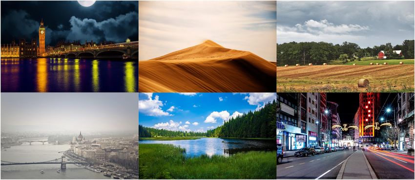
Bridge Composite and Real: Towards End-to-end Deep Image Matting                                                     3

                       (a)                                                         (b)
Fig. 1 (a) The comparison between representative end-to-end-matting methods in (i) and (ii) and our GFM in (iii). (b)
The comparison between existing matting datasets and our proposed benchmark as well as the comparison between existing
composition methods and our RSSN.

that can significantly reduce the domain gap arisen           alpha mattes (more than 1080 pixels in the shorter
from the discrepancies of resolution, sharpness, noise,       side), which are beneficial to train models with better
etc. Along with this, as shown in (ii) of Figure 1(b)         generalization on real-world images, and also suggests
COMP-Track, we propose a large-scale high-resolution          several new research problems which will be discussed
clean background dataset (BG-20k) without salient fore-       later.
ground objects, which can be used in generating high-            The contributions of this paper are four-fold:
resolution composite images. Extensive experiments show
                                                                  • We propose a novel model named GFM for end-
that the proposed composition route along with BG-
                                                              to-end image matting, which simultaneously generates
20k can reduce the generalization error by 60% and
                                                              global semantic segmentation and local alpha matte
achieve comparable performance as the model trained
                                                              without any priors as input but a single image.
using original natural images. It opens an avenue for
composition-based image matting since obtaining fore-             • We design a novel composition route RSSN to
ground images and alpha mattes are much easier than           reduce various kinds of discrepancies and propose a
those from original natural images by leveraging chroma       large-scale high-resolution background dataset BG-20k
keying.                                                       to serve as better candidates for generating high-quality
                                                              composite images.
    To fairly evaluate matting models’ generalization
ability on real-world images, we make the first attempt           • We construct a large-scale real-world images bench-
to establish a large-scale benchmark consists of 2000         mark to benefit training a better model with good gen-
high-resolution real-world animal images and 10,000 real-     eralization by its large scale, diverse categories, and
world portrait images along with manually carefully           high-quality annotations.
labeled fine alpha mattes. Comparing with previous                • Extensive experiments on the benchmark demon-
datasets (Xu et al., 2017; Qiao et al., 2020; Shen et al.,    strate that GFM outperforms state-of-the-art (SOTA)
2016) as in (i) and (ii) of Figure 1(b) ORI-Track which       matting models and can be a strong baseline for future
only provide foreground images or low-resolution inac-        research. Moreover, the proposed composition route RSSN
curate alpha mattes, our benchmark includes all the           demonstrates its value by reducing the generalization
high-resolution real-world original images and high-quality   error by a large margin.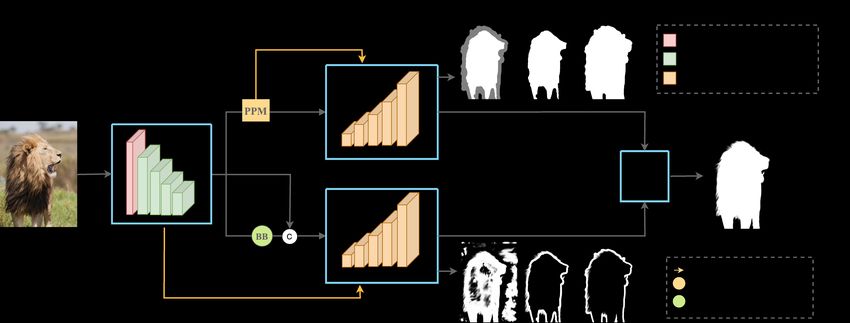
4                                                             Jizhizi Li1 , Jing Zhang1 , Stephen J. Maybank2 , Dacheng Tao1 ,

2 Related Work                                                   our GFM model only takes a single image as input
                                                                 without any priors; 2) the trimap branch in AdaMat-
2.1 Image Matting                                                ting aims to refine the input trimap, which is much
                                                                 easier than generating a global representation in our
Most classical image matting methods are using auxil-            case because the initial trimap actually serves as an at-
iary input like trimaps (Li et al., 2017; Sun et al., 2004;      tention mask for learning semantical features; 3) both
Levin et al., 2008; Chen et al., 2013; Levin et al., 2007).      the encoder and decoder structures of GFM are specif-
They sample or propagate foreground and background               ically designed for end-to-end matting, which differs
labels to the unknown areas based on local smoothness            from AdaMatting; and 4) we systematically investigate
assumptions. Recently, CNN-based methods improve                 the semantic-transition representations in the global de-
them by learning discriminative features rather than re-         coder and gain useful empirical insights.
lying on hand-crafted low-level color features (Xu et al.,
2017; Lu et al., 2019; Hou and Liu, 2019; Cai et al.,
2019; Tang et al., 2019). Deep Matting (Xu et al., 2017)         2.2 Matting Dataset
employed an encoder-decoder structure to extract high-
level contextual features. IndexNet (Lu et al., 2019) fo-        Existing matting datasets (Rhemann et al., 2009; Shen
cused on boundary recovery by learning the activation            et al., 2016; Xu et al., 2017; Zhang et al., 2019; Qiao
indices during down-sampling. However, trimap-based              et al., 2020) only contain foregrounds and a small num-
methods require user interaction, so are not likely to be        ber of annotated alpha mattes, e.g., 27 training images
deployed in automatic applications. Recently, Chen et            and 8 test images in alphamatting (Rhemann et al.,
al. (Chen et al., 2018) proposed an end-to-end model             2009), 431 training images and 50 test images in Comp-
that first predicted the trimap then carried out mat-            1k (Xu et al., 2017), and 596 training images and 50 test
ting. Zhang et al. (Zhang et al., 2019) also devised a           images in HAttMatting (Qiao et al., 2020). DAPM (Shen
two-stage model that first segmented the foreground or           et al., 2016) proposes 2,000 real-world portrait images
the background and then refined them with a fusion               but at fix-size and low-resolution, together with lim-
net. Both methods separate the process of segmenta-              ited quality alpha mattes generated by an ensemble
tion and matting in different stages, which may gen-             of existing matting models. In contrast to them, we
erate erroneous segmentation results that mislead the            propose a high-quality benchmark consists of 10,000
subsequent matting step. Qiao et al. (Qiao et al., 2020)         high-resolution real-world portrait images and 2,000 an-
employed spatial and channel-wise attention to inte-             imal images and manually annotated alpha matte for
grate appearance cues and pyramidal features while               each image. We empirically demonstrate that the model
predicting, however, the distinct appearance and se-             trained on our benchmark has a better generalization
mantics of foreground/background areas and transition            ability on real-world images than the one trained on
areas bring a lot of burden to a single-stage network            composite images.
and limit the quality of alpha matte prediction. Liu et
al. (Liu et al., 2020) proposed a network to perform hu-
man matting by predicting the coarse mask first, then            2.3 Image Composition
adopted a refinement network to predict a more de-
tailed one. Despite the necessity of stage-wise training         As the inverse problem of image matting and the typ-
and testing, a coarse mask is not enough for guiding             ical way of generating synthetic dataset, image com-
the network to refine the detail since the transition ar-        position plays an important role in image editing. Re-
eas are not defined explicitly.                                  searchers have been dedicated to improve the reality of
    In contrast to previous methods, we devise a novel           composite images from the perspective of color, light-
end-to-end matting model via multi-task learning, which          ing, texture compatibility, and geometric consistency
addresses the segmentation and matting tasks simul-              in the past years (Xue et al., 2012; Tsai et al., 2017;
taneously. It can learn both high-level semantic fea-            Chen and Kae, 2019; Cong et al., 2020). Xue et al. (Xue
tures and low-level structural features in a shared en-          et al., 2012) conducted experiments to evaluate how the
coder, benefiting the subsequent segmentation and mat-           image statistical measure including luminance, color
ting decoders collaboratively. One close related work            temperature, saturation, local contrast, and hue de-
with ours is AdaMatting (Cai et al., 2019), which also           termine the realism of a composite. Tsai et al. (Tsai
has a structure of a shared encoder and two decoders.            et al., 2017) proposed an end-to-end deep convolutional
There are several significant differences: 1) AdaMat-            neural network to adjust the appearance of the fore-
ting requires a coarse trimap as an extra input while            ground and background to be more compatible. Chen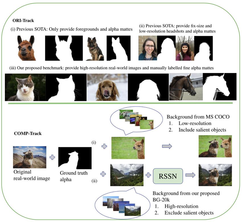
Bridge Composite and Real: Towards End-to-end Deep Image Matting                                                       5

Fig. 2 Diagram of the proposed Glance and Focus Matting (GFM) network, which consists of a shared encoder and two
separate decoders responsible for rough segmentation of the whole image and details matting in the transition area.

et al. (Chen and Kae, 2019) proposed a generative ad-           and explicitly model the collaboration. To this end, we
versarial network(GAN) architecture to learn geomet-            propose a novel Glance and Focus Matting network for
rically and color consistent in the composites. Cong et         end-to-end image matting as shown in Figure 2.
al. (Cong et al., 2020) contributed a large-scale image
harmonization dataset and a network using a novel do-
main verification discriminator to reduce the inconsis-
tency of foreground and background. Although they did           3.1 Shared Encoder
a good job in harmonizing the composites to be more
realistic, the domain gap still exists when fitting the
                                                                GFM has an encoder-decoder structure, where the en-
synthesis data into the matting model, the reason is a
                                                                coder is shared by two subsequent decoders. As shown
subjective agreed standard of harmonization by a hu-
                                                                in Figure 2, the encoder takes a single image as in-
man is not equivalent to a good training candidate for a
                                                                put and processes it through five blocks E0 ∼ E4 ,
machine learning model. Besides, such procedures may
                                                                where each reduces the resolution by half. We adopt the
modify the boundary of the foreground and result in
                                                                ResNet-34 (He et al., 2016) or DenseNet-121 (Huang
inaccuracy of the ground truth alpha matte. In this
                                                                et al., 2017) pre-trained on the ImageNet training set as
paper, we alternatively focus on generating composite
                                                                our backbone encoder. Specifically, for DenseNet-121,
images that can be used to reduce the generalization
                                                                we add a convolution layer to reduce the output fea-
error of matting models on natural images.
                                                                ture channels to 512.

3 GFM: Glance and Focus Matting Network

When tackling the image matting problem, we humans              3.2 Glance Decoder (GD)
first glance at the image to quickly recognize the salient
rough foreground or background areas and then focus             The glance decoder aims to recognize the easy semantic
on the transition areas to distinguish details from the         parts and leave the others as unknown areas. To this
background. It can be formulated as a rough segmenta-           end, the decoder should have a large receptive field to
tion stage and a matting stage roughly. Note that these         learn high-level semantics. As shown in Figure 2, we
two stages may be intertwined that there will be feed-          symmetrically stack five blocks D4G ∼ D0G as the de-
back from the second stage to correct the erroneous de-         coder, each of which consists of three sequential 3 × 3
cision at the first stage, for example, in some ambiguous       convolutional layers and an upsampling layer. To en-
areas due to the protective coloration of animals or oc-        large the receptive field further, we add a pyramid pool-
clusions. To mimic the human experience and empower             ing module (PPM) (Zhao et al., 2017; Liu et al., 2019)
the matting model with proper abilities at both stages,         after E4 to extract global context, which is then con-
it is reasonable to integrate them into a single model          nected to each decoder block DiG via element-wise sum.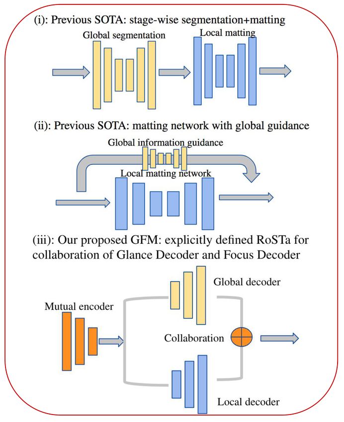
6                                                               Jizhizi Li1 , Jing Zhang1 , Stephen J. Maybank2 , Dacheng Tao1 ,

   Loss Function The training loss for the glance de-              3.4 RoSTa: Representation of Semantic and Transition
coder is a cross-entropy loss LCE defined as follows:              Areas
          C
          X                                                        To investigate the impact of the representation format
                Gcg log Gcp ,

LCE = −                                                  (2)
          c=1
                                                                   of the supervisory signal in our GFM, we adopt three
                                                                   kinds of Representations of Semantic and Transition
where Gcp ∈ [0, 1] is the predicted probability   for cth          areas (RoSTa) as the bridge to link GD and FD.
class, Gcg ∈ {0, 1} is the ground truth label. Theoutput
of GD is a two- or three-channel (C = 2 or 3) class prob-           – GFM-TT We use the classical 3-class trimap T as
ability map depends on the semantic-transition repre-                 the supervisory signal for GD, which is generated by
sentation, which will be detailed in Section 3.4.                     dilation and erosion from ground truth alpha matte
                                                                      with a kernel size of 25. We use the ground truth
                                                                      alpha matte α in the unknown transition areas as
3.3 Focus Decoder (FD)                                                the supervisory signal for FD.
                                                                    – GFM-FT We use the 2-class foreground segmen-
As shown in Figure 2, FD has the same basic structure                 tation mask F as the supervisory signal for GD,
as GD, i.e., symmetrically stacked five blocks D4F ∼                  which is generated by the erosion of ground truth
D0F . Different from GD, which aims to do roughly se-                 alpha matte with a kernel size of 50 to ensure the
mantic segmentation, FD aims to extract details in the                left foreground part is correctly labeled. In this case,
transition areas where low-level structural features are              the area of I (α > 0) − F is treated as the transition
very useful. Therefore, we use a bridge block (BB) (Qin               area, where I (·) denotes the indicator function. We
et al., 2019) instead of the PPM after E4 to leverage                 use the ground truth alpha matte α in the transition
local context in different receptive fields. Specifically, it         area as the supervisory signal for FD.
consists of three dilated convolutional layers. The fea-            – GFM-BT We use the 2-class background segmen-
tures from both E4 and BB are concatenated and fed                    tation mask B as the supervisory signal for glance
into D4F . We follow the U-net (Ronneberger et al., 2015)             decoder, which is generated by dilation of ground
style and add a shortcut between each encoder block Ei                truth alpha matte with kernel size as 50 to ensure
and the decoder block DiF to preserve fine details.                   the left background part is correctly labeled. In this
    Loss Function The training loss for FD (LF D ) is                 case, the area of B −I (α > 0) is treated as the tran-
composed of an alpha-prediction loss LTα and a Lapla-                 sition area. We use the ground truth alpha matte α
cian loss LTlap in the unknown transition areas (Xu et al.,           in the transition area as the supervisory signal for
2017), i.e.,                                                          FD.
LF D = LTα + LTlap .                                     (3)

Following (Xu et al., 2017), the alpha loss LTα is cal-            3.5 Collaborative Matting (CM)
culated as absolute difference between ground truth α
and predicted alpha matte αF in the unknown transi-        As shown in Figure 2, CM merges the predictions from
tion region. It is defined as follows:                     GD and FD to generate the final alpha prediction. Specif-
           q                                               ically, CM follows different rules when using different
                                 2
                                                           RoSTa as described in Section 3.4. In GFM-TT, CM re-

               αi − αiF × WiT + ε2
       P
  T      i
Lα =                P      T
                                       ,            (4)    places the transition area of the prediction of GD with
                       i Wi                                the prediction of FD. In GFM-FT, CM adds the pre-
where i denotes pixel index, Wi ∈ {0, 1} denotes whether dictions from GD and FD to generate the final alpha
                                T

pixel i belongs to the transition region or not. We add    matte. In GFM-BT, CM subtracts the prediction of FD
ε = 10−6 for computational stability. Following (Hou       from the prediction of GD as the final alpha matte. In
and Liu, 2019), the Laplacian loss LTlap is defined as the this way, GD takes charge of recognizing rough fore-
L1 distance between the Laplacian pyramid of ground        ground and background by learning global semantic
truth and that of prediction.                              features, and FD is responsible for matting details in
                                                           the unknown areas by learning local structural features.
                 5
        X       X                                          Such task decomposition and specifically designed par-
LTlap =     WiT      (Lapk (αi ) − Lapk (αiF ) 1 ,     (5)
                                                           allel decoders make the model simpler than the two-
         i      k=1
                                                           stage ones in (Chen et al., 2018; Zhang et al., 2019).
           k
where Lap denotes the kth level of the Laplacian pyra-     Besides, both decoders are trained simultaneously that
mid. We use five levels in the Laplacian pyramid.          the loss can be back-propagated to each of them via the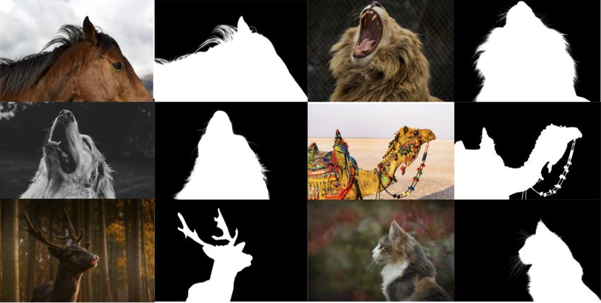
Bridge Composite and Real: Towards End-to-end Deep Image Matting                                                      7

CM module. In this way, our model enables interaction        Noise discrepancy. To address these issues, we propose
between both decoders that the erroneous prediction          a new composition route named RSSN and a large-scale
can be corrected in time by the responsible branch. Ob-      high-resolution background dataset named BG-20k.
viously, it is expected to be more effective than the two-
stage framework, where the erroneous segmentation in
the first stage could not be corrected by the subsequent     4.1 Resolution Discrepancy and Semantic Ambiguity
one and thus mislead it.
                                                             In the literature of image matting, the background im-
    Loss Function The training loss for collaborative
                                                             ages used for composition are usually chosen from exist-
matting (LCM ) consists of an alpha-prediction loss Lα ,
                                                             ing benchmarks for image classification and detection,
a Laplacian loss Llap , and a composition loss Lcomp ,
                                                             such as MS COCO (Lin et al., 2014) and PASCAL VOC
i.e.,
                                                             (Everingham et al., 2010). However, these background
LCM = Lα + Llap + Lcomp .                             (6)    images are in low-resolution and may contain salient
                                                             objects, causing the following two types of discrepan-
Here Lα and Llap are calculated according to Eq. (4)         cies.
and Eq. (5) but in the whole alpha matte. Following
                                                             1. Resolution Discrepancy: A typical image in MS
(Xu et al., 2017), the composition loss (Lcomp ) is calcu-
                                                                COCO (Lin et al., 2014) or Pascal VOC (Evering-
lated as the absolute difference between the composite
                                                                ham et al., 2010) has a resolution about 389 × 466,
images based on the ground truth alpha and the pre-
                                                                which is much smaller compared to the high-resolution
dicted alpha matte by referring to (Levin et al., 2007).
                                                                foreground images in matting dataset such as Compsition-
It can be defined as follows:
               q                                                1k (Xu et al., 2017). The resolution discrepancy be-
          P                       2
                 C(αi ) − C(αiCM ) + ε2                         tween foreground and background images will result
             i
Lcomp =                                   ,            (7)      in obvious artifacts as shown in Figure 3(b).
                         N                                   2. Semantic ambiguity: Images in MS COCO (Lin
where C (·) denotes the composited image, αCM is the            et al., 2014) and Pascal VOC (Everingham et al.,
predicted alpha matte by CM, and N denotes the num-             2010) are collected for classification and object de-
ber of pixels in the alpha matte.                               tection tasks, which usually contain salient objects
    To sum up, the final loss used during training is           from different categories, including various animals,
calculated as the sum of LCE , LF D and LCM , i.e.,             human, objects. Directly pasting the foreground im-
                                                                age with such background images will result in se-
L = LCE + LF D + LCM .                                (8)       mantic ambiguity for end-to-end image matting. For
                                                                example, as shown in Figure 3(b), there is a dog in
                                                                the background which is beside the leopard in the
                                                                composite image. Training with such images will
4 RSSN: A Novel Composition Route
                                                                mislead the model to ignore the background ani-
                                                                mal, i.e., probably learning few about semantics but
Since labeling alpha matte of real-world natural images
                                                                more about discrepancies.
is very laborious and costly, a common practice is to
generate large-scale composition images from a few of            To address these issues, we collect a large-scale high-
foreground images and the paired alpha mattes (Xu            resolution dataset named BG-20k to serve as good back-
et al., 2017). The prevalent matting composition route       ground candidates for composition. We only selected
is to paste one foreground with various background im-       those images whose shortest side has at least 1080 pixels
ages by alpha blending according to Eq. (1). However,        to reduce the resolution discrepancy. Moreover, we re-
since the foreground and background images are usually       moved those images containing salient objects to elim-
sampled from different distributions, there will be a lot    inate semantic ambiguity. The details of constructing
of composition artifacts in the composite images, which      BG-20k are presented as follows.
lead to a large domain gap between the composition im-
                                                             1. We collected 50k high-resolution (HD) images us-
ages and natural ones. The composition artifacts may
                                                                ing the keywords such as HD background, HD view,
mislead the model by serving as cheap features, result-
                                                                HD scene, HD wallpaper, abstract painting, interior
ing in overfitting on the composite images and produc-
                                                                design, art, landscape, nature, street, city, moun-
ing large generalizing errors on natural images. In this
                                                                tain, sea, urban, suburb from websites with open
section, we systematically analyze the factors that cause
                                                                licenses1 , removed those images whose shorter side
the composition artifacts including Resolution discrep-
ancy, Semantic ambiguity, Sharpness discrepancy, and          1   https://unsplash.com/ and https://www.pexels.com/
8 Jizhizi Li1 , Jing Zhang1 , Stephen J. Maybank2 , Dacheng Tao1 ,
Fig. 3 Comparison of different image composition methods. (a) Original natural image. (b) Composite with background from
MS COCO (Lin et al., 2014) with foreground computed by (Levin et al., 2007). (c) Composite with background from our
proposed BG-20k by alpha blending of original image directly. (d) Composite with background from our proposed BG-20k
with foreground computed by (Levin et al., 2007). (e) Composite with large-aperture effect.
sition route. More examples of BG-20k are presented in
Figure 4 and the supplementary video.
4.2 Sharpness Discrepancy
In photography, it is usually to use a large aperture and
focal length to capture a sharp and salient foreground
image within the shallow depth-of-field, thus highlight-
Fig. 4 Some examples from our BG-20k dataset. ing it from the background context, which is usually
blurred due to the out-of-focus effect. An example is
shown in Figure 3(a), where the leopard is the cen-
has less than 1080 pixels and resized the left images ter of interest and the background is blurred. Previous
to have 1080 pixels at the shorter side while keeping composition methods dismiss this effect, producing a
the original aspect ratio. The average resolution of domain gap of sharpness discrepancy between the com-
images in BG-20k is 1180 × 1539; posite images and natural photos. Since we target the
2. We removed duplicate images by a deep matching image matting task, where the foregrounds are usually
model (Krizhevsky et al., 2012). We adopted YOLO- salient in the images, thereby we investigate this effect
v3 (Redmon and Farhadi, 2018) to detect salient in our composition route. Specifically, we simulate it by
objects and then manually double-checked to make adopting the averaging filter in OpenCV with a kernel
sure each image has no salient objects. In this way, size chosen from 20, 30, 40, 50, 60 randomly to blur the
we built BG-20k containing 20,000 high-resolution background images. Since some natural photos may not
clean images; have blurred backgrounds, we only use this technique
3. We split BG-20k into a disjoint training set (15k) in our composition route with a probability of 0.5. An
and validation set (5k). example is shown in Figure 3(e), where the background
is chosen from BG-20k and blurred using the averag-
ing filter. As can be seen, it has a similar style to the
An composition example using the background im-
original image in (a).
age from BG-20k is shown in Figure 3(c) and Figure 3(d).
In (c), we use the foreground image computed by multi-
plying ground truth alpha matte with the original im- 4.3 Noise Discrepancy
age for alpha blending, in (d), we use the foreground
image computed by referring to the method in (Levin Since the foreground and background come from dif-
et al., 2007) for alpha blending. As can be seen, there ferent image sources, they may contain different noise
are obvious color artifacts in (c) that blends both colors distributions. This is another type of discrepancy, which
of foreground and background in the fine details. The will mislead the model to search noise cues during train-
composite image in (d) is much more realistic than that ing, resulting in overfitting. To address this discrepancy,
in (c). Therefore, we adopt the method in (Levin et al., we adopt BM3D (Dabov et al., 2009) to remove noise
2007) for computing foreground images in our compo- in both foreground and background images in RSSN.Bridge Composite and Real: Towards End-to-end Deep Image Matting 9
Furthermore, we add Gaussian noise with a standard Pipeline 1: The Proposed Composition
deviation of 10 to the composite image such that the Route: RSSN
noise distributions in both foreground and background Input: The matting dataset M containing |M |
areas are the same. We find that it is effective in im- images and the background image set BG-20k
proving the generalization ability of trained models. Output: The composite image set C
1: for each i ∈ [1, |M |] do
2: if there are original images in M , e.g. AM-2k,
4.4 The RSSN Composition Route PM-10k then
3: Sample an original image Ii ∈ M
We summarize the proposed composition route RSSN 4: Sample the paired alpha matte αi ∈ M
5: Compute the foreground Fi given (Ii , αi ) (Levin
in Pipeline 1. The input of the pipeline is the matting et al., 2007)
dataset, e.g., AM-2k and PM-10k as will be introduced 6: else
in Section 5.1, DIM (Xu et al., 2017), or DAPM (Shen 7: Sample a foreground image Fi ∈ M
et al., 2016), and the proposed background image set 8: Sample the paired alpha matte αi ∈ M
9: end if
BG-20k. If the matting dataset provides original im- 10: for each k ∈ [1, K ] do
ages, e.g., AM-2K and DAPM (Shen et al., 2016), we 11: Sample a background candidate Bik ∈ BG-20k
compute the foreground from the original image given 12: if random() < 0.5 then
the alpha matte by referring to (Levin et al., 2007). 13: Fi = Denoise(Fi ) //denoising by BM3D (Dabov
et al., 2009)
We random sample K background candidates from BG- 14: Bik = Denoise(Bik )
20k for each foreground for data augmentation. We 15: end if
set K = 5 in our experiments. For each foreground 16: if random() < 0.5 then
image and background image, we carried out the de- 17: Sample a blur kernel size r ∈ {20, 30, 40, 50, 60}
18: Bik = Blur(Bik , r) // the averaging filter
noising step with a probability of 0.5. To simulate the 19: end if
effect of large-aperture, we carried out the blur step 20: Alpha blending: Cik = Fi × αi + Bik × (1 − αi )
on the background image with a probability of 0.5, 21: if random() < 0.5 then
where the blur kernel size was randomly sampled from 22: Cik = AddGaussianN oise(Cik )
23: end if
{20, 30, 40, 50, 60}. We then generated the composite 24: end for
image according to the alpha-blending equation Eq. (1). 25: end for
Finally, with a probability of 0.5, we added Gaussian
noise to the composite image to ensure the foreground
and background areas have the same noise distribution. testing bed for real-world image matting. We also setup
To this end, we generate a composite image set that has two evaluation tracks for different purposes. Details are
reduced many kinds of discrepancies, thereby narrowing presented as follows.
the domain gap with natural images.
5 Empirical Studies 5.1.1 AM-2k
5.1 Benchmark for Real-world Image Matting AM-2k (Animal Matting 2,000 Dataset) consists of 2,000
high-resolution images collected and carefully selected
Due to the tedious process for generating manually la- from websites with open licenses. AM-2k contains 20
beled high-quality alpha mattes, the amount of real- categories of animals including: alpaca, antelope, bear,
world matting dataset is very limited, most previous camel, cat, cattle, deer, dog, elephant, giraffe, horse,
methods adopted composite dataset such as Comp-1k (Xu kangaroo, leopard, lion, monkey, rabbit, rhinoceros, sheep,
et al., 2017), HATT-646 (Qiao et al., 2020) and LF (Zhang tiger, zebra, each with 100 real-world images of vari-
et al., 2019) for data augmentation. However, as dis- ous appearance and diverse backgrounds. We ensure the
cussed in Section. 4.4, the composition artifacts caused shorter side of the images is more than 1080 pixels. We
by such convention would result in large domain gap then manually annotate the alpha mattes using open-
when adapting to real-world images. To fill this gap, source image editing software, e.g., Adobe Photoshop,
we propose two large-scale high-resolution real-world GIMP, etc. We randomly select 1,800 out of 2,000 to
image matting datasets AM-2k and PM-10k, consists form the training set and the rest 200 as the validation
of 2,000 animal images and 10,000 portrait images re- set. Some examples and their ground truth are shown
spectively, along with the high-quality manually labeled in Figure 5. Please note that AM-2k has no privacy or
alpha mattes to serve as an appropriate training and license issue and is ready to release to public.10 Jizhizi Li1 , Jing Zhang1 , Stephen J. Maybank2 , Dacheng Tao1 ,
evaluate matting methods on real-world images in the
validation set same as the ORI-Track to validate their
generalization ability.
Experiments were carried out on two tracks of the
AM-2k and PM-10k datasets: 1) to compare the pro-
posed GFM with SOTA methods, where we trained and
evaluated them on the ORI-Track; and 2) to evaluated
the side effect of domain gap caused by previous com-
position method and the proposed composition route,
where we trained and evaluated GFM and SOTA meth-
Fig. 5 Some examples from our AM-2k dataset. The alpha ods on the COMP-Track, i.e., COMP-COCO, COMP-
matte is displayed on the right of the original image.
BG20k, and COMP-RSSN, respectively.
5.1.2 PM-10k
5.2 Evaluation Metrics and Implementation Details
PM-10k (Portrait Matting 10,000 Dataset) consists of
10,000 high-resolution images collected and carefully 5.2.1 Evaluation Metrics
selected from websites with open licenses. We ensure
Following the common practice in (Rhemann et al.,
PM-10k includes images with multiple postures and di-
2009; Zhang et al., 2019; Xu et al., 2017), we used
verse backgrounds. We process the images and generate
the mean squared error (MSE), the sum of absolute
the ground truth alpha mattes as in AM-2k. We then
differences (SAD), gradient (Grad.), and connectivity
split 9,500 of 10,000 to serve as training set and 500 as
(Conn.) as the major metrics to evaluate the quality of
validation set.
alpha matte predictions. Note that the MSE and SAD
metrics evaluate the pixel-wise difference between the
5.1.3 Benchmark Tracks prediction and ground truth alpha matte, while the gra-
dient and connectivity metrics favor clear details. Be-
To benchmark the performance of matting models 1) sides, we also use some auxiliary metrics such as Mean
trained and tested both on real-world images; and 2) Absolute Difference (MAD), SAD-TRAN (SAD in the
trained on composite images and tested on real-world transition areas), SAD-FG (SAD in the foreground ar-
images, we setup the following two evaluation tracks. eas), and SAD-BG (SAD in the background areas) to
comprehensively evaluate the quality of alpha matte
ORI-Track (Original Images Based Track) is set to per- predictions. While MAD evaluates the average quan-
form end-to-end matting tasks on the original real-world titative difference regardless of the image size, SAD-
images. The ORI-Track is the primary benchmark track. TRAN, SAD-FG, and SAD-BG evaluate SAD in dif-
ferent semantic areas, respectively. In addition, we also
COMP-Track (Composite Images Based Track) is set compared the model complexity of different methods
to investigate the influence of domain gap in image mat- in terms of the number of parameters, computational
ting. As discussed before, the composite images have a complexity, and inference time.
large domain gap with natural images due to the com-
position artifacts. If we can reduce the domain gap 5.2.2 Implementation Details
and learn a domain-invariant feature representation,
we can obtain a model with better generalization. To During training, we used multi-scale augmentation sim-
this end, we set up this track by making the first at- ilar to (Xu et al., 2017). Specifically, we cropped each
tempt towards this research direction. Specifically, we of the selected images with size from {640 × 640, 960 ×
construct the composite training set by alpha-blending 960, 1280 × 1280} randomly, resized the cropped image
each foreground with five background images from the to 320 × 320, and randomly flipped it with a probabil-
COCO dataset (Lin et al., 2014) (denoted as COMP- ity of 0.5. The encoder of GFM was initialized with the
COCO) and our BG-20k dataset (denoted as COMP- ResNet-34 (He et al., 2016) or DenseNet-121 (Huang
BG20K), or adopting the composition route RSSN pro- et al., 2017) pre-trained on the ImageNet dataset. GFM
posed in Section 4.4 based our BG-20K (denoted as was trained on two NVIDIA Tesla V100 GPUs. The
COMP-RSSN). Moreover, unlike previous benchmarks batch size was 4 for DenseNet-121 (Huang et al., 2017)
that evaluate matting methods on composite images (Xu and 32 for ResNet-34 (He et al., 2016). For the COMP-
et al., 2017; Zhang et al., 2019; Qiao et al., 2020), we Track, we composite five training images by using fiveBridge Composite and Real: Towards End-to-end Deep Image Matting 11
Table 1 Results on the ORI-Track and COMP-Track of AM-2k. (d) stands for DenseNet-121 Huang et al. (2017) backbone,
(r) stands for ResNet-34 He et al. (2016) backbone. Representations of T T , F T and BT can refer to Section 3.4.
Dataset AM-2k
Track ORI
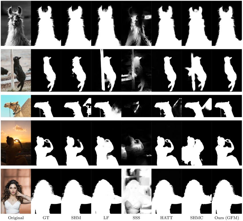
Method SHM LF SSS HATT SHMC GFM-TT(d) GFM-FT(d) GFM-BT(d) GFM-TT(r) GFM-FT(r) GFM-BT(r)
SAD 17.81 36.12 552.88 28.01 61.50 10.27 12.74 12.74 10.89 12.58 12.61
MSE 0.0068 0.0116 0.2742 0.0055 0.0270 0.0027 0.0038 0.0030 0.0029 0.0037 0.0028
MAD. 0.0102 0.0210 0.3225 0.0161 0.0356 0.0060 0.0075 0.0075 0.0064 0.0073 0.0074
Grad. 12.54 21.06 60.81 18.29 37.00 8.80 9.98 9.13 10.00 10.33 9.27
Conn. 17.02 33.62 555.97 17.76 60.94 9.37 11.78 10.07 9.99 11.65 9.77
SAD-TRAN 10.26 19.68 88.23 13.36 35.23 8.45 9.66 8.67 9.15 9.34 8.77
SAD-FG 0.60 3.79 401.66 1.36 10.93 0.57 1.47 3.07 0.77 1.31 2.84
SAD-BG 6.95 12.55 62.99 13.29 15.34 1.26 1.61 1.00 0.96 1.93 1.00
Track COMP-COCO COMP-BG20K COMP-RSSN
Method SHM GFM-TT(d) GFM-TT(r) SHM GFM-TT(d) GFM-TT(r) SHM GFM-TT(d) GFM-FT(d) GFM-BT(d) GFM-TT(r)
SAD 182.70 46.16 30.05 52.36 25.19 16.44 23.94 19.19 20.07 22.82 15.88
MSE 0.1017 0.0223 0.0129 0.02680 0.0104 0.0053 0.0099 0.0069 0.0072 0.0078 0.0049
MAD 0.1061 0.0273 0.0176 0.03054 0.0146 0.0096 0.0137 0.0112 0.0118 0.0133 0.0092
Grad. 64.74 20.75 17.22 22.87 15.04 14.64 17.66 13.37 12.53 12.49 14.04
Conn. 182.05 45.39 29.19 51.76 24.31 15.57 23.29 18.31 19.08 19.96 15.02
SAD-TRAN 25.01 17.10 15.21 15.32 13.35 12.36 12.63 12.10 12.12 12.06 12.03
SAD-FG 23.26 8.71 4.74 3.52 3.79 1.46 4.56 4.37 3.47 5.20 1.15
SAD-BG 134.43 20.36 10.1 33.52 8.05 2.62 6.74 2.72 4.48 5.56 2.71
Dataset PM-10k
Track ORI
Method SHM LF SSS HATT SHMC GFM-TT(d) GFM-FT(d) GFM-BT(d) GFM-TT(r) GFM-FT(r) GFM-BT(r)
SAD 16.64 37.51 687.16 22.66 57.85 11.89 12.76 13.45 11.52 12.10 13.34
MSE 0.0069 0.0152 0.3158 0.0038 0.0291 0.0041 0.0044 0.0039 0.0038 0.0037 0.0036
MAD. 0.0097 0.0152 0.3958 0.0131 0.0340 0.0069 0.0074 0.0078 0.0067 0.0070 0.0078
Grad. 14.54 21.82 69.72 15.16 37.28 12.9 12.61 13.22 13.07 14.68 13.09
Conn. 16.13 36.92 691.08 11.95 57.86 11.24 12.15 11.37 10.83 11.38 10.54
SAD-TRAN 8.53 16.36 63.64 9.32 23.04 7.80 7.81 7.80 8.00 8.82 8.02
SAD-FG 0.74 11.63 240.02 0.79 13.08 1.65 0.69 3.98 0.97 0.93 3.88
SAD-BG 7.37 9.52 383.49 12.54 21.72 2.44 4.26 1.67 2.54 2.35 1.44
Track COMP-COCO COMP-BG20K COMP-RSSN
Method SHM GFM-TT(d) GFM-TT(r) SHM GFM-TT(d) GFM-TT(r) SHM GFM-TT(d) GFM-FT(d) GFM-BT(d) GFM-TT(r)
SAD 168.75 61.69 34.58 34.06 21.54 20.29 22.02 18.15 19.68 21.80 13.84
MSE 0.0926 0.0309 0.0165 0.0160 0.0088 0.0086 0.0094 0.0071 0.0078 0.0075 0.0049
MAD 0.0960 0.0355 0.0198 0.0194 0.0125 0.0118 0.0126 0.0106 0.0114 0.0126 0.0080
Grad. 53.83 32.00 18.73 23.02 19.21 16.85 18.65 18.12 17.50 16.97 14.44
Conn 167.28 61.26 33.96 33.7 20.97 19.67 21.61 17.57 19.25 19.09 13.15
SAD-TRAN 23.86 17.69 11.21 12.85 11.82 10.26 10.6 10.78 10.61 10.38 9.00
SAD-FG 21.27 17.42 13.99 9.66 5.31 7.56 5.24 2.66 3.58 5.74 1.32
SAD-BG 123.62 26.59 9.37 11.55 4.41 2.46 6.19 4.70 5.48 5.68 3.52
different backgrounds for each foreground on-the-fly dur- rows of Table 1. GFM-TT, GFM-FT, and GFM-BT
ing training. It took about two days to train GFM for denote the proposed GFM model with different RoSTa
500 epochs on ORI-Track and 100 epochs for COMP- as described in Section 3.4. (d) and (r) stand for us-
Track. The learning rate was fixed to 1 × 10⁻⁴ for the ing DenseNet-121 (Huang et al., 2017) and ResNet-
ORI-Track and 1 × 10⁻⁵ for the COMP-Track. 34 (He et al., 2016) as the backbone encoder, respec-
For baseline methods LF (Zhang et al., 2019) and tively. There are several empirical findings from Table 1.
SSS (Aksoy et al., 2018), we used the official codes First, SSS (Aksoy et al., 2018) achieved the worst
released by authors. For SHM (Chen et al., 2018), performance with a large foreground/background SAD
HATT (Qiao et al., 2020) and SHMC (Liu et al., error of 401.66 or 383.49 compare with others, the rea-
2020) with no public codes, we re-implemented them son is twofold. 1) They adopt the pre-trained Deeplab-
according to the papers. For SHMC (Liu et al., 2020) ResNet-101 (Chen et al., 2017) model as the semantic
which does not specify the backbone network, we used feature extractor to calculate affinities. The pre-trained
ResNet-34 (He et al., 2016) for a fair comparison. These model may generate limited representative features on
models were trained using the training set on the ORI- the high-resolution matting dataset which degrade the
Track or COMP-Track. performance. 2) This method aims to extract all the se-
mantic regions in the image while other matting meth-
ods are trained to extract only the salient animal or
5.3 Quantitative and Subjective Evaluation portrait foreground. Second, SHMC using global guid-
ance (Liu et al., 2020) and stage-wise method LF (Zhang
5.3.1 Results on the ORI-Track et al., 2019) perform better than SSS (Aksoy et al.,
2018) in all evaluation metrics. However, the SAD er-
We benchmarked several SOTA methods (Chen et al., rors in the transition area dominate the total errors,
2018; Zhang et al., 2019; Aksoy et al., 2018; Qiao et al., which is 35.23 and 19.68, 23.04 and 16.36 for AM-2k and
2020; Liu et al., 2020) on the ORI-Track of AM-2k PM-10k, respectively. The reason is that both of them
and PM-10k. The results are summarized in the top have not explicitly define the transition area, thereby12 Jizhizi Li1 , Jing Zhang1 , Stephen J. Maybank2 , Dacheng Tao1 ,
the matting network has limited ability to distinguish soy et al., 2018), and LF (Zhang et al., 2019), GFM can
the details in the transition area when it needs seg- be trained in a single stage and the collaboration mod-
ment foreground and background using the same net- ule acts as an effective gateway to back-propagate mat-
work at the same time. It can also be confirmed by the ting errors to the responsible branch adaptively. Sec-
scores of Grad. and Conn. Third, HATT(Qiao et al., ond, compared with methods that adopt global guid-
2020) performs better than SHMC (Liu et al., 2020) ance, e.g., HATT (Qiao et al., 2020) and SHMC (Liu
and LF (Zhang et al., 2019) in terms of SAD error in et al., 2020), GFM explicitly model the end-to-end mat-
the transition area and foreground area because the at- ting task into two separate but collaborate sub-tasks by
tention module it adopted can provide better global ap- two distinct decoders. Moreover, it uses a collaboration
pearance filtration. However, using a single network to module to merge the predictions according to the def-
model both the foreground and background areas and inition of RoSTa, which explicitly defines the role of
the transition areas of plentiful details makes it hard to each decoder.
powerful representative features for both areas, result- From Figure 6, we can find similar observations.
ing in large SAD errors especially in the background SHM (Chen et al., 2018), LF (Zhang et al., 2019), and
areas as well as large Grad. and Conn. errors. SSS (Aksoy et al., 2018) fail to segment some fore-
Fourth, SHM (Chen et al., 2018) performs the best ground parts, implying inferiority of its stage-wise net-
among all the SOTA methods. It reduces the SAD er- work structure, since they do not distinguish the fore-
ror in the transition area from 13.36 to 10.26 for AM- ground/background and the transition areas explicitly
2k, 9.32 to 8.53 for PM-10k, and the SAD error in the in the model. It is hard to balance the role of semantic
background area from 13.29 to 6.95 for AM-2k, 12.54 segmentation for the former and matting details for the
to 7.37 for PM-10k compared with HATT (Qiao et al., latter, which requires global semantic and local struc-
2020). We believe the improvement credits to the ex- tural features, respectively. HATT (Qiao et al., 2020)
plicit definition of RoSTa (i.e., the trimap) and the and SHMC (Liu et al., 2020) struggle to obtain clear de-
PSPNet (Zhao et al., 2017) used in the first stage which tails in the transition areas since the global guidance is
has a good semantic segmentation capability. However, helpful for recognizing the semantic areas while being
SHM (Chen et al., 2018) still has large error in the less useful for matting of details. Compared to them,
background area due to its stage-wise pipeline, which our GFM achieves the best results owing to the ad-
will accumulate the segmentation error into the matting vantage of a unified model, which deals with the fore-
network. Last, compare with all the SOTA methods, ground/background and transition areas using separate
our GFM outperforms them in all evaluation metrics, decoders and optimizes them in a collaborative manner.
achieving the best performance by simultaneously seg- More results of GFM can be found in the supplemen-
menting the foreground and background and matting tary video.
on the transition areas, no matter which kind of RoSTa
it uses. For example, it achieves the lowest SAD error 5.3.2 Results on the COMP-Track
in different areas, i.e. 8.45 v.s. 10.26 for AM-2k, 7.80
v.s. 8.53 for PM-10k in the transition area, 0.57 v.s. We evaluated SHM (Chen et al., 2018), the best per-
0.60 for AM-2k, 0.69 v.s. 0.74 for PM-10k in the fore- formed SOTA method and our GFM with two different
ground area, and 0.96 v.s. 6.95 for AM-2k, 1.44 v.s. 7.37 backbones on the COMP-Track of AM-2k and PM-10k
for PM-10k in the background area compared with the including COMP-COCO, COMP-BG20K, and COMP-
previous best method SHM (Chen et al., 2018). The RSSN. The results are summarized in the bottom rows
results of using different RoSTa are comparable, espe- of Table 1, from which we have several empirical find-
cially for FT and BT, since they both define two classes ings. First, when training matting models using im-
in the image for segmentation by the Glance Decoder. ages from MS COCO dataset (Lin et al., 2014) as back-
GFM using TT as the RoSTa performs the best due grounds, GFM performs much better than SHM (Chen
to its explicit definition of the transition area as well et al., 2018), i.e, 46.16 and 30.05 v.s. 182.70 for AM-2k,
as the foreground and background areas. We also tried 61.69 and 34.58 v.s. 168.75 for PM-10k in terms of whole
two different backbone networks, ResNet-34 (He et al., image SAD, confirming the superiority of the proposed
2016) and DenseNet-121 (Huang et al., 2017). Both of model over the two-stage one for generalization. Sec-
them achieve better performance compared with other ond, GFM using ResNet-34 (He et al., 2016) performs
SOTA methods. better than using DenseNet-121 (Huang et al., 2017),
The reason of GFM’s superiority over other methods perhaps due to the more robust representation ability
can be explained as follows. First, compared with stage- of residual structure in ResNet-34 (He et al., 2016).
wise methods, e.g., SHM (Chen et al., 2018), SSS (Ak- Third, when training matting models using backgroundBridge Composite and Real: Towards End-to-end Deep Image Matting 13
images from the proposed BG-20k dataset, the errors of Model Ensemble Since we propose three different
all the methods are significantly reduced, especially for RoSTa for GFM, it is interesting to investigate their
SHM (Chen et al., 2018), i.e., from 182.70 to 52.36 for complementary. To this end, we calculated the result by
AM-2k, or 168.75 to 34.06 for PM-10k, which mainly a model ensemble which takes the median of the alpha
attributes to the reduction of SAD error in the back- predictions from three models as the final prediction. As
ground area, i.e., from 134.43 to 33.52 for AM-2k and shown in Table 2, the result of the model ensemble is
123.62 to 11.55 for PM-10k. There is the same trend better than any single one, i.e., 9.21 v.s. 10.27 for GFM-
for GFM(d) and GFM(r). These results confirm the TT(d), 9.92 v.s. 10.89 for GFM-TT(r), confirming the
value of our BG-20k, which helps to reduce resolution complementary between different RoSTa.
discrepancy and eliminate semantic ambiguity in the Hybrid-resolution Test For our GFM, we also
background area. proposed a hybrid-resolution test strategy to balance
Fourth, when using the proposed RSSN for train- GD and FD. Specifically, we first fed a down-sampled
ing, the errors can be reduced further for SHM (Chen image to GFM to get an initial result. Then, we used
et al., 2018), i.e., from 52.36 to 23.94 for AM-2k and the full resolution image as input and only used the
34.06 to 22.02 for PM-10k, from 25.19 to 19.19 and predicted alpha matte from FD to replace the initial
21.54 to 18.15 for GFM(d), and from 16.44 to 15.88 prediction in the transition areas. For simplicity, we de-
and 20.19 to 13.84 for GFM(r). The improvement is note the down-sampling ratio at each step as d1 and
attributed to the composition techniques in RSSN: 1) d2 , which are subject to d1 ∈ {1/2, 1/3, 1/4}, d2 ∈
we simulate the large-aperture effect to reduce sharp- {1/2, 1/3, 1/4}, and d1 ≤ d2 . Their results are listed in
ness discrepancy; and 2) we remove the noise of fore- Table 2. A smaller d1 increases the receptive field and
ground/background and add noise to the composite im- benefits the Glance Decoder, while a larger d2 benefits
age to reduce noise discrepancy. Note that the SAD the Focus Decoder with clear details in high-resolution
error of SHM (Chen et al., 2018) has dramatically re- images. Finally, we set d1 = 1/3 and d2 = 1/2 for a
duced about 87% from 182.70 to 23.93 for AM-2k or trade-off.
168.75 to 22.02 for PM-10k when using RSSN com-
pared with the traditional composition method based
on MS COCO dataset, which is even comparable with 5.5 Ablation Study
the one obtained by training using original images, i.e.,
17.81 for AM-2k and 16.64 for PM-10k. It demonstrates
that the proposed composition route RSSN can sig- Table 3 Ablation study of GFM on AM-2k.
nificantly narrow the domain gap and help to learn
down-invariant features. Last, We also conducted ex- Track ORI
Method SAD MSE MAD Grad Conn
periments by using different RoSTa in GFM(d) on COMP- GFM-TT(d) 10.27 0.0027 0.0060 8.80 9.37
RSSN, their results have a similar trend to those on the GFM-TT(r) 10.89 0.0029 0.0064 10.00 9.99
GFM-TT(r2b) 10.24 0.0028 0.0060 8.65 9.33
ORI-TRACK. GFM-TT-SINGLE(d) 13.79 0.0040 0.0081 13.45 13.04
GFM-TT-SINGLE(r) 15.50 0.0040 0.0091 14.21 13.15
GFM-TT(d) excl. PPM 10.86 0.0030 0.0064 9.91 9.92
GFM-TT(d) excl. BB 11.27 0.0035 0.0067 9.33 10.40
5.4 Model Ensemble and Hybrid-resolution Test GFM-TT(r) excl. PPM 11.90 0.0035 0.0070 10.50 11.07
GFM-TT(r) excl. BB 11.29 0.0032 0.0066 9.59 10.43
Track COMP-RSSN
GFM-TT(d) 25.19 0.0104 0.0146 15.04 24.31
GFM-TT(d) w/ blur 21.37 0.0081 0.0124 14.31 20.50
Table 2 Model Ensemble and Hybrid-resolution Test on AM- GFM-TT(d) w/ denoise 22.95 0.0090 0.0134 14.37 22.10
GFM-TT(d) w/ noise 19.87 0.0075 0.0116 13.22 18.97
2k. GFM-TT(d) w/ RSSN 19.19 0.0069 0.0112 13.37 18.31
Track Ensemble
Method SAD MSE MAD Grad. Conn.
GFM-ENS(d) 9.21 0.0021 0.0054 8.00 8.16
GFM-ENS(r) 9.92 0.0024 0.0058 8.82 8.92 5.5.1 Results on the ORI-Track
Track Hybrid
d1 d2 SAD MSE MAD Grad. Conn.
1/2 1/2 12.57 0.0041 0.0074 9.26 11.75 To further verify the benefit of the designed structure of
1/3 1/2 10.27 0.0027 0.0060 8.80 9.37 GFM, we conducted ablation studies on several variants
1/3 1/3 11.58 0.0028 0.0067 11.67 10.67 of GFM on the ORI-Track of AM-2k, including 1) moti-
1/4 1/2 13.23 0.0045 0.0078 10.00 12.26
1/4 1/3 14.65 0.0047 0.0086 12.46 13.68
vated by Qin et.al (Qin et al., 2019), in GFM encoder
1/4 1/4 17.29 0.0055 0.0102 16.50 16.28 when using ResNet-34 (He et al., 2016) as the back-
bone, we modified the convolution kernel of E0 fromYou can also read