Nonlinear effects in 4D-Var - Nonlinear Processes in Geophysics
←
→
Page content transcription
If your browser does not render page correctly, please read the page content below
Nonlin. Processes Geophys., 25, 713–729, 2018
https://doi.org/10.5194/npg-25-713-2018
© Author(s) 2018. This work is distributed under
the Creative Commons Attribution 4.0 License.

Nonlinear effects in 4D-Var
Massimo Bonavita, Peter Lean, and Elias Holm
European Centre for Medium-Range Weather Forecasts, Shinfield Park, Reading, RG2 9AX, UK

Correspondence: Massimo Bonavita (massimo.bonavita@ecmwf.int)

Received: 14 March 2018 – Discussion started: 6 April 2018
Revised: 10 August 2018 – Accepted: 21 August 2018 – Published: 19 September 2018

Abstract. The ability of a data assimilation system to deal         (NWP) applications becomes computationally unaffordable
effectively with nonlinearities arising from the prognostic         and, even if it were possible, the interpretation and usefulness
model or the relationship between the control variables and         of the result in the case of multi-modal error distributions be-
the available observations has received a lot of attention in       come unclear in a deterministic analysis context (Lorenc and
theoretical studies based on very simplified test models. Less      Payne, 2007).
work has been done to quantify the importance of nonlin-               In order to make the variational problem computationally
earities in operational, state-of-the-art global data assimila-     tractable and mathematically well posed, simplifications are
tion systems. In this paper we analyse the nonlinear effects        required. One idea would be to reduce the dimensionality
present in ECMWF 4D-Var and evaluate the ability of the             of the control vector used in the minimisation, for exam-
incremental formulation to solve the nonlinear assimilation         ple limiting it to the subspace where dynamical instabili-
problem in a realistic NWP environment. We find that non-           ties develop during the data assimilation cycle (Trevisan and
linearities have increased over the years due to a combination      Uboldi, 2004; Carrassi et al., 2008; Trevisan et al., 2010).
of increased model resolution and the ever-growing impor-           Another approach starts from recognising that the use of a
tance of observations that are nonlinearly related to the state.    linear model and linear observation operators leads to strictly
Incremental 4D-Var is well suited for dealing with these non-       quadratic cost functions, which brings two major benefits:
linear effects, but at the cost of increasing the number of outer   (a) it guarantees the convergence of the minimisation al-
loop relinearisations. We then discuss strategies for accom-        gorithm to the global minimum and (b) it allows the use
modating the increasing number of sequential outer loops in         of efficient, gradient-based iterative minimisation algorithms
the tight schedules of operational global NWP.                      (Fisher, 1998). This consideration has spurred research in
                                                                    NWP applications of variational methods towards perturba-
                                                                    tive solution algorithms, where the full nonlinear minimisa-
                                                                    tion problem is approximated as a series of quadratic cost
1   Introduction                                                    functions obtained by repeated linearisations around progres-
                                                                    sively more accurate guess values of the solution. This idea,
The importance of nonlinear effects has been recognised             based on the general Gauss–Newton method for the solution
since the early days of the development of 4D-Var (e.g. Gau-        of nonlinear least squares problems (Björck, 1996), was first
thier, 1992; Rabier and Courtier, 1992; Miller et al., 1994;        introduced in the meteorological literature by Courtier, Thé-
Pires et al., 1996). The presence of nonlinearities in either       paut and Hollingsworth (1994) (CTH in the following) as
the model or the observations can potentially cause signifi-        “Incremental 4D-Var”. In that paper the main stated objec-
cant deviations from the usual Gaussian distribution assumed        tive of incremental 4D-Var was the reduction of the compu-
to describe observation and background errors in the defini-        tational costs of full 4D-Var in order to make it feasible for
tion of the 4D-Var cost function. This in turn translates into a    operational application. Its ability to deal with weak nonlin-
more complex topology of the cost function and the potential        earities was also noted and subsequently investigated in sim-
for multiple minima (e.g. Pires et al., 1996; Hoteit, 2008).        plified models, particularly in relation to the length of the as-
In these conditions, finding the global minimum of the 4D-          similation window and the global convergence properties of
Var cost function for realistic numerical weather prediction

Published by Copernicus Publications on behalf of the European Geosciences Union & the American Geophysical Union.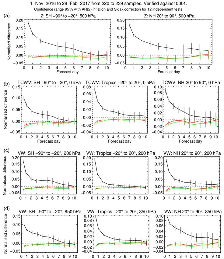
714                                                                           M. Bonavita et al.: Nonlinear effects in 4D-Var

the algorithm (e.g. Tanguay et al., 1995; Laroche and Gau-         important components of the observing system used opera-
thier, 1998).                                                      tionally at ECMWF (Geer et al., 2017) and it is thus impor-
   After the operational implementation of incremental 4D-         tant to understand the capabilities and limitations of 4D-Var
Var at ECMWF (Rabier et al., 2000) and, later, in other ma-        to deal with these type of nonlinearities.
jor global NWP Centres (Kadowaki, 2005; Rosmond and                   Given the motivation above, the remainder of this paper is
Xu, 2006; Gauthier et al., 2007; Rawlins et al., 2007) the         organised as follows. In Sect. 2, we briefly review the incre-
possibility arose to address in realistic NWP settings still       mental 4D-Var algorithm in order to highlight the hypotheses
open questions about the limits of applicability of 4D-Var         underlying the tangent linear approximation and the math-
in nonlinear situations. A series of studies (Andersson et al.,    ematical basis of the outer loop iterations. In Sect. 3 evi-
2005; Radnòti et al., 2005; Trémolet, 2004, 2007) conducted        dence of nonlinear effects in current ECMWF 4D-Var is pre-
with the ECMWF Integrated Forecasting System (IFS) pro-            sented, from both an observational and a model perspective.
vided answers to some of these questions in the context of         In Sect. 4, we evaluate how effective incremental 4D-Var is
the ECMWF operational system of the time. These studies            in dealing with both observation and model nonlinearities.
emphasised the importance of the consistency between the           Section 5 addresses the question of how important the ability
nonlinear and linearised evolution of the analysis increments      to run outer loops is in the current ECMWF data assimilation
during the assimilation window for the global convergence          system, in terms of both analysis and forecast skill. These re-
of the incremental 4D-Var. This, in turn, was shown to re-         sults and their implication for data assimilation strategy at
quire the availability of accurate linearised models, and the      ECMWF and elsewhere are discussed in Sect. 6.
need to run inner and outer loops with not too large discrep-
ancies in terms of spatial resolution and time step (a ratio
of three between the outer and inner loop resolutions was          2   Algorithmic aspects
found to give satisfactory results). As there is no guarantee
                                                                   The aim of variational data assimilation is to determine the
of global convergence of the incremental 4D-Var algorithm,
                                                                   model trajectory that best fits in a least square sense the ob-
the aforementioned studies also stressed the importance of
                                                                   servations available during a given time window. This con-
regularly re-evaluating the nonlinearity issues in future oper-
                                                                   cept naturally leads to the formulation of the standard strong
ational systems.
                                                                   constraint 4D-Var cost function:
   From the time of these investigations, the operational
ECMWF IFS has changed considerably. From the perspec-                        1
                                                                   J (x 0 ) = (x 0 − x b )T B−1 (x 0 − x b )
tive of the validity of the linearity assumptions in the incre-              2
mental formulation, two changes are particularly relevant:                     1X K                  T
                                                                                      y k − Gk (x 0 ) R−1

(a) the increase in resolution at both outer loop and inner                  +                             k y k − Gk (x 0 )
                                                                               2 k=0
loop level and (b) the introduction of a very large number of
humidity, cloud and precipitation-sensitive satellite observa-               = JB (x 0 ) + JO (x 0 ) .                           (1)
tions in the analysis system (Geer et al., 2017). In terms of
spatial resolution, the effective grid spacing has gone from       In Eq. (1) x 0 is the control vector at the start of the assimila-
approx. 40 km (TL511, i.e. spectral triangular truncation 511      tion window; x b and B are the background and its expected
with a linear grid) to approx. 9 km (TCo1279, spectral trian-      error covariance matrix; y k and Rk are the set of observations
gular truncation 1279 with a cubic grid; see Malardel et al.,      presented to the analysis in the k sub-window and their ex-
2016, for more details), for the 4D-Var outer loops, and from      pected error covariances; and Gk is a generalised observation
approx. 130 km (TL159) to approx. 50 km (TL399) for the            operator (or forward model) that produces the model equiva-
inner loops. Thus, nonlinearities are expected to play a larger    lents of the observations y k by first integrating the prognostic
role in the current IFS, also in view of the fact that the ratio   model from t0 to tk and then applying the standard observa-
between the resolutions of the outer and inner loops of the        tion operator Hk to the propagated fields, i.e.:
minimisation has increased from approx. 3.2 to 5.5. In terms       Gk = Hk ◦ Mt0 →tk .                                           (2)
of observation usage, the increase in the number and influ-
ence of humidity, cloud and precipitation-sensitive observa-       The formulation (1) represents the general nonlinear
tions can also be expected to expose nonlinear effects con-        weighted least square solution of the assimilation problem
nected to the way their observation operators respond to fore-     using the forecast model as a strong constraint. Problem (1)
casted humidity and precipitation structures. Some of these        cannot however be solved efficiently by standard optimal
issues were already described at the time of the introduction      control methods for realistic numerical weather prediction
of the “all-sky” framework for the assimilation of microwave       (NWP) data assimilation systems, given the size of the con-
imagers sensitive to humidity and precipitation (Bauer et al.,     trol vector x 0 (O(109 )). A possible solution, first proposed in
2010), but at that time the number and influence of these ob-      CTH (1994), under the name of “Incremental 4D-Var”, is to
servation types on the 4D-Var analysis was relatively small.       simplify the solution of Eq. (1) through the application of an
Currently, however, all-sky observations are one of the most       approximated form of the Gauss–Newton method (Lawless

Nonlin. Processes Geophys., 25, 713–729, 2018                                www.nonlin-processes-geophys.net/25/713/2018/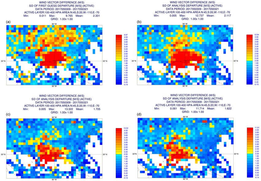
M. Bonavita et al.: Nonlinear effects in 4D-Var                                                                                      715

et al., 2005; Gratton et al., 2007). This consists of approxi-          et al., 2017b). The other aspect affecting the validity of the
mating the minimisation of the nonlinear cost function (1) as           TL approximation relies on an implicit linearity assumption
a sequence of minimisations of linear, quadratic cost func-             of both the forecast model and the observation operator in
tions defined in terms of perturbations around a sequence of            a neighbourhood of the reference trajectory. Experience at
progressively more accurate trajectories (i.e. nonlinear model          ECMWF indicates that there is a clear sensitivity of both
integrations). The cost function linearised around a guess tra-         the linearised observation operator and the linearised model
jectory x g can be expressed as an exact quadratic problem in           to the linearisation state (e.g. Bauer et al., 2010; Janisková
terms of the increment at the initial time δx 0 :                       and Lopez, 2013). It is thus relevant to revisit the roles of
                                                                        model and observation nonlinearities in the current opera-
              1          g      T               g                      tional ECMWF 4D-Var implementation and to validate the
                δx 0 + x 0 − x b B−1 δx 0 + x 0 − x b

J (δx 0 ) =
              2                                                         effectiveness of the incremental 4D-Var method in dealing
                   K
                1X                                                      with these nonlinearities.
              +       (d k − Gk (δx 0 ))T R−1
                                           k (d k − Gk (δx 0 ))            Other, possibly less well-known, sources of nonlinearities
                2 k=0
                                                                        in the ECMWF incremental 4D-Var formulation stem from
            = JB (δx 0 ) + JO (δx 0 ) .                     (3)         the variational quality control (VarQC) of the observations
                             g                                         and the nonlinear change of variable used for the humidity
In Eq. (3) d k = y k − Gk x 0 are the observation departures
                                                                        analysis. The VarQC algorithm is based on the Huber norm
around the latest model trajectory and Gk = Hk Mt0 →tk is the
                                                                        (Tavolato and Isaksen, 2015) and has the effect of making the
linearisation of the generalised observation operator around
                                                                        observation error matrix R a function of the current depar-
the defined trajectory.
                                                                        ture d k and thus of the reference state. However, as it is cur-
   In the observation part of the cost function, the so-called
                                                                        rently applied to conventional observation only, its impact on
“tangent linear (TL) approximation” has been made in going
                                                                        the linearity of the minimisation is limited. The other source
from Eq. (1) to Eq. (3):
                                                                        of nonlinearity arises from the nonlinear change of variable
                             g                                         used in the humidity analysis (Hólm et al., 2002), which im-
y k − Gk (x 0 ) = y k − Gk x 0 + δx 0 =
                                                                      plies that also the JB part of the cost function in Eq. (3) is not
                g                 1        ∂Gk                         a purely quadratic function of the initial increment δx 0 and,
 = y k − Gk x 0 − Gk (δx 0 ) − (δx 0 )T             (δx 0 )
                                   2         ∂x x g                     consequently, the gradient of JB with respect to the initial
                                                                        increment is not linear in δx 0 . Consistently with the incre-

                                 g
 − O kδx 0 k3 ≈ y k − Gk x 0 − Gk (δx 0 ) .                 (4)
                                                                        mental 4D-Var philosophy, this is handled by a linear update
                                                                        of the humidity control variable in the quadratic cost func-
   In the Taylor expansion in Eq. (4), terms of O kδx 0 k2

                                                                        tion (3), followed by a nonlinear update of the humidity field
and higher are neglected (note that if Eq. 4 is exactly satis-          at the outer loop level to provide the initial state for the new
fied, then Eq. 3 is equivalent to Eq. 1). This approximation,           reference trajectory. The nonlinear effects connected with the
as first noted in Lawless et al. (2005), is equivalent to the           humidity control variable are intimately linked with the us-
standard approximation used in the Gauss–Newton optimi-                 age of the all-sky observations, which provide the vast major-
sation algorithm, i.e. neglecting the second-order derivatives          ity of humidity sensitive observations, and will be discussed
of Gk in the Hessian of the cost function:                              in that context.
                    K
                    X                           XK  ∂Gk
  2
∇ J =B    −1
                +             T
                          (Gk )    R−1
                                    k (Gk ) −    k=0  ∂x x g            3     Evidence of nonlinear effects in 4D-Var
                    k=0
                                  g
       R−1
        k  y k − Gk x 0                  ≈                              3.1    The role of the model
                 K
                 X
       B−1 +           (Gk )T R−1
                               k (Gk ) .                          (5)   Model nonlinearities affect the 4D-Var solution in two main
                 k=0                                                    ways. First, the more nonlinear the high-resolution trajectory
                                                                        solution is, the spatially noisier the low-resolution interpo-
The validity of the tangent linear approximation is thus based          lated linearisation state for the 4D-Var inner loops becomes.
on whether either the increments δx 0 are in some sense                 This roughness of the interpolated trajectory increases when
small or the dependence of the linearisation of Gk (i.e. Gk =           differences between the time steps and resolutions of the in-
Hk Mt0 →tk ) on the reference trajectory is negligible. Con-            ner loops and the trajectory become larger. Second, the tan-
cerning the first aspect, we only note here that the size of            gent linear evolution differs more from the nonlinear solution
analysis increments is, to first order, a linear function of ob-        as nonlinearities increase. One measure of the degree of non-
servation departures. Thus, the sizes of departures need to             linearity (Rabier and Courtier, 1992) is to take the difference
be small with respect to the observation and background er-             between the nonlinearly and linearly evolved increments in
rors used in the analysis update for the TL approximation to            the last minimisation,
hold (the interested reader can find further details in Bonavita

www.nonlin-processes-geophys.net/25/713/2018/                                        Nonlin. Processes Geophys., 25, 713–729, 2018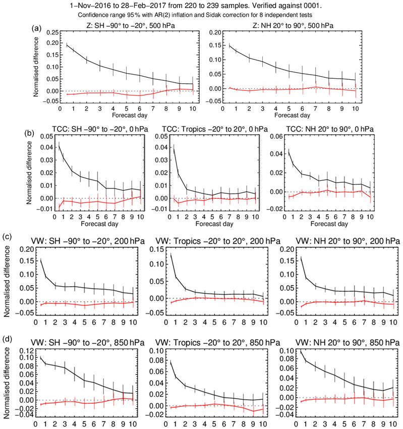
716                                                                                   M. Bonavita et al.: Nonlinear effects in 4D-Var


Figure 1. Globally averaged profiles of historical ECMWF 4D-Var differences M x n−1 + δx n − M x n−1 + Mδx n in the last minimi-
sation 9 h into the 12 h assimilation window for vorticity (a) and divergence (b) in 2004, 2008, 2013 and 2017. Over the years, the resolution
and number of inner and outer loops have increased from 60-level TL511/TL95-TL159 in 2004 to 137-level TCo1279/TL255-TL319-TL399
in 2017.


M x n−1 + δx n − M x n−1 + Mδx n ,                              (6)       1 XN                         1 XN
                                                                              i=0
                                                                                  Gk (x0 + δxi ) =                 G (x )
                                                                                                               i=0 k 0
                                                                          N                            N
and the globally averaged profile of the standard deviation of                1 XN                                      XN
                                                                            +      i=0
                                                                                         G k (δx i ) = G k (x 0 ) + G k   i=0
                                                                                                                              δx i
this quantity is shown in Fig. 1 for selected years from 2004                 N
to 2017. Over the years, there has been an increase in the res-             ∼
                                                                            = Gk (x0 ) .                                                  (7)
olution of the trajectory and the inner loops and the gap in
resolution between the two has increased. This has resulted              Figure 2a–d show the relationship between the ensemble
in increased differences, which we interpret as increased non-           mean model equivalent value and the model equivalent val-
linearity due to the combination of increased model resolu-              ues in the unperturbed control member for different obser-
tion and resolution differences between the inner loop and the           vation types. For observations sensitive to tropospheric tem-
trajectory. One way to counteract the nonlinearity that comes            perature, such as the Advanced Microwave Sounding Unit A
with resolution increases is to shorten the length of the as-            (AMSU-A) channel 6 (Fig. 2a) and radiosonde temperature
similation window. This can be achieved either by very short             observations (Fig. 2b), a strong linear relationship holds, in-
windows or by the use of overlapping assimilation windows.               dicating that nonlinear effects in the observation operators
In this second case the reduction in nonlinearity is realised            are negligible. However, operators associated with observa-
by reducing the size of the analysis increments δx n as each             tions sensitive to humidity and cloud show more significant
new window will start from a first guess trajectory that has             nonlinear behaviour. For example, the Advanced Technology
already seen the observations in the overlapped part of the              Microwave Sounder (ATMS) channel 20 (Fig. 2c) is sensi-
window.                                                                  tive to humidity and the Advanced Microwave Scanning Ra-
                                                                         diometer 2 (AMSR-2) channel 11 (Fig. 2d) is sensitive to
3.2   The role of the observations                                       cloud liquid water.

The significance of nonlinearities in the observation opera-
tors can be estimated using statistics from the Ensemble of              4    Dealing with nonlinearities through the incremental
Data Assimilations (EDA, Isaksen et al., 2010) system which                   approach
is run operationally at ECMWF. Each ensemble member is
initialised using a perturbed model state with perturbations             The incremental approach to 4D-Var (CTH, 1994) reduces
drawn from a distribution with zero mean. For linear obser-              the resolution of the inner loops to make the solution more af-
vation operators and Gaussian perturbations, the ensemble                fordable. Observation departures are calculated at high reso-
mean of the model equivalents provided by the observation                lution and then the high-resolution trajectory is truncated and
operators is expected to be close to the unperturbed control             interpolated to the resolution of the inner loop for each time
member (in fact, it should match it exactly in the limit of              step of the low-resolution minimisation (Trémolet, 2004). At
infinite ensemble size):                                                 the end of the minimisation, the increments are projected
                                                                         back to the high resolution and added to the previous tra-
                                                                         jectory at the start of the assimilation window. This process

Nonlin. Processes Geophys., 25, 713–729, 2018                                       www.nonlin-processes-geophys.net/25/713/2018/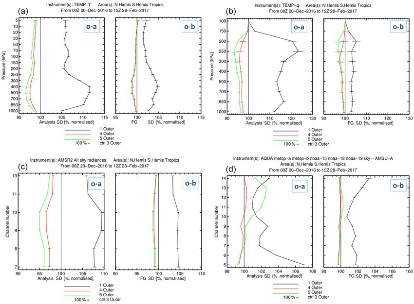
M. Bonavita et al.: Nonlinear effects in 4D-Var                                                                                    717

Figure 2. Ensemble mean G(x) (x axis) against control member G(x) for (a) AMSU-A channel 6 in clear-sky locations, (b) radiosonde
temperature, (c) ATMS channel 20 (clear-sky) and (d) ASMR-2 channel 11 observations (all-sky).

is repeated for all minimisations, which can be at different            details of the operational 4D-Var set-up). It can be seen that
resolutions, starting with the lowest resolution to capture the         each minimisation improves the fit between the model trajec-
larger scales and increasing the resolution in later minimisa-          tory and the observations. However, the standard deviation in
tions to extract more detailed information from the observa-            each nonlinear trajectory step is consistently higher than that
tions (Veerse and Thépaut, 1998).                                       at the end of the previous minimisation. This is to be ex-
                                                                        pected because of the resolution difference between nonlin-
4.1   Impact diagnostics in observation space                           ear and linearised models and also due to the fact that nonlin-
                                                                        ear processes cannot be represented by the linear model and
Bauer et al. (2010) discussed how the difference in departures          operators used in the minimisations.
at the end of each minimisation step, and those in the subse-              Figure 4 plots the correlation coefficient and standard de-
quent nonlinear trajectory step (i.e. δdk = dknon-linear −dklinear ),   viation of these differences at each outer loop, demonstrating
indicate the presence of nonlinearities in the system. Fig-             that nonlinearities become smaller at each successive outer
ure 3 shows the standard deviation of the guess departures              loop. For “linear” observation types such as radiosonde tem-
at each stage of the operational 4D-Var for AMSR-2 chan-                perature and AMSU-A channel 6, the nonlinearities are less
nel 10, which is sensitive to water vapour (see Sect. 5 for

www.nonlin-processes-geophys.net/25/713/2018/                                      Nonlin. Processes Geophys., 25, 713–729, 2018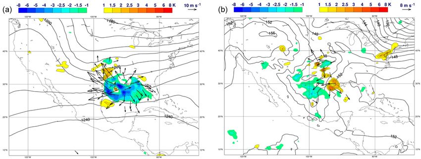
718                                                                                 M. Bonavita et al.: Nonlinear effects in 4D-Var

Figure 3. Standard deviation of departures for AMSR-2 channel           Figure 4. Taylor diagram showing the correlation (azimuthal an-
10 in the nonlinear trajectories (circles) and at the end of the min-   gle) and standard deviation (distance from the origin) of the dif-
imisation of the linearised cost function (triangles) for each outer    ferences in the departures (K) between the nonlinear trajectory and
loop of 4D-Var. Note how the nonlinear and linearised departure         linear minimisation steps for each outer loop. Results are shown for
standard deviations should coincide in the linear case. The average     satellite brightness temperature observations (ASMU-A channel 6,
background error standard deviation in observation space for this       ATMS channel 20) and radiosonde temperature observations.
type of observation is 3.4 K. Results from a single cycle from the
ECMWF operational assimilation system.

                                                                        sis increments is seen to gradually decrease for successive
significant than for ATMS channel 20 (which is sensitive to             outer loop iterations, more rapidly in the stratosphere for
humidity).                                                              vorticity. After five outer loop iterations, the magnitude of
   As expected, the departures for observations sensitive to            the analysis increments appears to asymptote to a relatively
cloud and humidity show increased nonlinear impacts. Fig-               small value for temperature throughout the atmospheric col-
ure 5 shows results from AMSR-2 channel 11 categorised                  umn (1Ta ≈ 0.05 K), and for vorticity in the stratosphere
using estimates of cloudiness from both the observations                and mesosphere (1voa ≈ 10−7 s−1 for model levels greater
and the model fields (Geer and Bauer, 2011). It can be seen             than 70). On the other hand, incremental 4D-Var does not
that the linear assumption holds less well for observations in          seem to have fully converged for vorticity in the troposphere.
cloudy regions compared to those in areas of clear sky.                 This is confirmed by the longitudinal averages of the anal-
                                                                        ysis increments produced by the first and last outer loops
4.2   Impact diagnostics in model space                                 for temperature, vorticity and humidity, which are shown in
                                                                        Fig. 7. It is apparent how the last outer loop iteration still
A clear indicator of the success or otherwise of the incre-             manages to produce non-negligible increments for the tropo-
mental strategy is the size of the analysis increments pro-             spheric wind and humidity fields (middle and bottom rows in
duced by the linearised cost function (3) during successive             Fig. 7), as a result of the increased presence of nonlinear ob-
outer loop iterations. For a well-behaved incremental 4D-               servations and the increased nonlinearity of the relevant me-
Var converging towards the solution of the nonlinear cost               teorology (e.g. organised convection and baroclinic instabil-
function (1), successive analysis increments are expected               ity). This suggests that increasing the number of outer loops
to become smaller, reflecting the hypothesis that successive            from the current operational value of three up to at least five
first guess trajectories provide increasingly accurate descrip-         can lead to a better use of available observations and, ulti-
tions of the flow. This hypothesis is supported by the ex-              mately, more accurate analyses and forecasts. An interesting
perimental results shown in Fig. 6, where we present the                side aspect of this investigation has been to highlight the rel-
vertical profiles of the standard deviations of the analysis            atively large analysis increments produced by 4D-Var in the
increments of vorticity (left panel) and temperature (right             mesosphere (i.e. above model level 20 in the plots). This is
panel) from a multi-incremental 4D-Var experiment with five             due to a combination of relatively inaccurate model dynam-
outer loops (in this experiment the outer loop resolution is            ics due to sponge layer effects and the scarcity of observa-
TCo399, approx. 30 km, and the inner loop resolutions are               tional constraints in this part of the atmosphere (the highest
TL95/TL159/TL255/TL255/TL255, approx. 210, 125, and                     peaking channels from current microwave sounders are only
80 km; more details in Table 1). The magnitude of the analy-            marginally sensitive to this upper atmospheric layer).

Nonlin. Processes Geophys., 25, 713–729, 2018                                     www.nonlin-processes-geophys.net/25/713/2018/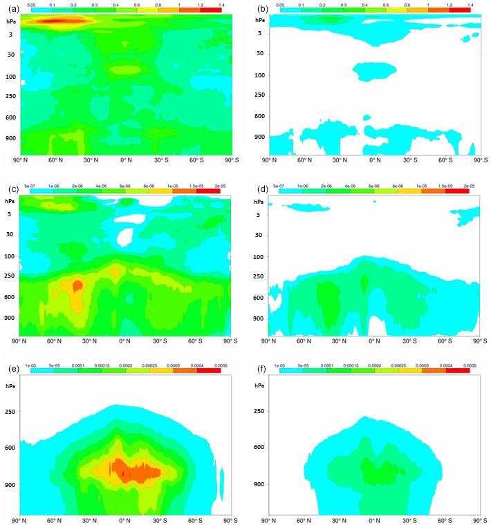
M. Bonavita et al.: Nonlinear effects in 4D-Var 719
Table 1. Resolution and number of outer loop iterations for the sensitivity experiments discussed in Sect. 5. TCo399 means IFS model
integrations with spectral triangular truncation 399 and a cubic octahedral reduced Gaussian grid. TLXXX mean IFS model integrations
carried out at spectral triangular truncation XXX on a linear reduced Gaussian grid. All minimisations are performed using the full physics
tangent linear and adjoint models.
Experiment Resolution of Number of Resolution of
outer loop outer loops minimisations
Reference TCo399 3 TL95/TL159/TL255
1 outer loop experiment TCo399 1 TL255
4 outer loop experiment TCo399 4 TL95/TL159/TL255/TL255
5 outer loop experiment TCo399 5 TL95/TL159/TL255/TL255/TL255
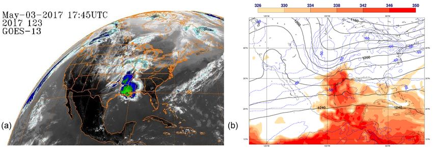
panel) is characteristic of this type of event (Maddox, 1980):
a strong warm, moist southerly flow from the Gulf of Mex-
ico is taking place in the lower troposphere, in the region
ahead of an upper level trough. The combination of strong
warm and moist air advection in the lower levels with vortic-
ity advection aloft leads to a situation conducive to intense
organised convection in a region along the Texas–Louisiana
coast, starting at around 13:00 UTC on the 3 May 2017 and
lasting until approx. 06:00 UTC on 4 May 2017. Forecasting
the intensity and location of convection is notoriously diffi-
cult and the ECMWF analysis increments (Fig. 9) show that
the operational 4D-Var makes significant changes to the first
guess fields throughout the atmospheric column. In particu-
lar, the analysis appears to adjust the strength of the convec-
tive system through a significant cooling at the top of the tro-
posphere and associated enhancement of the divergent wind
field (Fig. 9, left panel). In the boundary layer (Fig. 9, right
Figure 5. As Fig. 4 but showing results from AMSR-2 channel 11 panel), the analysis increments show more spatial variability,
categorising observations by those in clear-sky regions and those but the main signal of localised warming and convergence of
impacted by cloud. the wind field in the direction of movement of the convective
system are apparent.
The magnitude of the analysis increments in the case stud-
4.3 A test case ied here (up to ∼ 8 K for temperature, ∼ 30 m s−1 for wind)
is more than an order of magnitude larger than their aver-
An informative example of the effectiveness of incremental age standard deviations: thus, significant nonlinear effects
4D-Var in dealing with nonlinear error evolution in active are expected in the assimilation update. This is confirmed
weather systems is described in the following test case of in Fig. 10 where we show the standard deviation of the first
organised convection in the southern United States. These guess and analysis departures from wind observations in the
high-impact weather phenomena are particularly interesting 100–400 hPa layer for the first guess and the one, three, five
from a data assimilation perspective because: (1) they have outer loop analyses over the 09:00 to 21:00 UTC assimilation
been shown to be potential precursors of significant forecast window of 3 May 2017 (All experiments are performed at the
“busts” in downstream regions, Europe in particular (Rod- operational TCo1279 resolution, approx. 9 km grid spacing,
well et al., 2013); and (2) they occur in probably the most using IFS cycle 43R3). It is visually apparent that the anal-
densely observed region of the world, thus allowing a more ysed trajectories are better able to fit the observations with
in-depth look into the ability of the assimilation system to increasing number of outer loops: the area-averaged stan-
make effective use of the observations. dard deviation of the innovations decreases from 2.301 m s−1
In the case described here, large-scale organised convec- in the first guess trajectory to 2.117, 1.705 and 1.622 m s−1
tion with the satellite signature of a mesoscale convective in the one, three and five outer loop analysis trajectories,
complex (Fig. 8, left panel), was forming in the southern respectively. No further improvements were seen with fur-
US coastal plains in the local evening hours of 3 May 2017, ther increases in the outer loop count, which points to resid-
continuing for most of the night. The synoptic situation, as ual model deficiencies, either in terms of spatial resolution
depicted by the ECMWF operational analysis (Fig. 8, right
www.nonlin-processes-geophys.net/25/713/2018/ Nonlin. Processes Geophys., 25, 713–729, 2018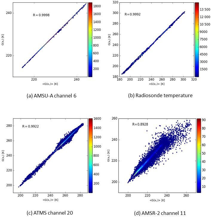
720                                                                                   M. Bonavita et al.: Nonlinear effects in 4D-Var

Figure 6. Vertical profiles of the globally averaged standard deviation of the analysis increments produced by successive outer loop iterations
for vorticity (a) and temperature (b). Values have been averaged over a 1-month period. The assimilation experiment has been run with an
outer loop resolution corresponding to a cubic octahedral reduced Gaussian grid with spectral truncation 399 (TCo399, approx. 30 km grid
spacing), and inner loop resolutions corresponding to linear reduced resolution Gaussian grids at spectral truncations TL95/159/255/255/255,
corresponding to approx. 210/120/80 km grid spacing.

and/or model errors; or missing representativeness errors in              vational dataset used in operations at ECMWF has been as-
the specified observation errors. We note that the wind ob-               similated. The number of inner loop iterations in the minimi-
servations whose departures are shown in the plots in Fig. 10             sations is not prescribed, because minimisations stop when
come from the US radiosonde network and from aircraft ob-                 a convergence criterion based on the information content of
servations, which implies that linear observation operators               the minimisation is reached (Fisher, 2003). Convergence is
are used. Thus, the nonlinear effects seen in the plots arise             usually reached in approx. 30 iterations, and this number has
exclusively from nonlinearities in the evolution of model per-            been found not to be sensitive to resolution and number of
turbations in the assimilation window.                                    outer loop relinearisations. A hard stopping criterion of 50 it-
                                                                          erations is also present, but in all the experiments reported
                                                                          here it was never reached. An additional point to note is that
5     Results from cycling data assimilation experiments                  all the experiments have at least one minimisation performed
                                                                          at the highest resolution (i.e. TL255). Thus, differences in
The diagnostics presented in Sect. 4 showed that increasing               analysis and forecast performance cannot be attributed to ei-
the number of outer loop iterations in the ECMWF 4D-Var                   ther insufficient resolution in the minimisation or incomplete
helps to reduce the magnitude of nonlinearities in the analy-             convergence.
sis and suggests that it can lead to a better use of available ob-
servations, in particular those that are nonlinearly related to           5.1   Analysis skill – full observing system
the model state. The next step is then to verify that these find-
ings are confirmed in a cycled data assimilation environment              A standard way to evaluate the skill of the analyses produced
as close as is computationally affordable to the operational              by a cycling data assimilation system is to look at the statis-
ECMWF assimilation system. To this end a series of data as-               tics of observation minus analysis (o − a) departures and ob-
similation experiments has been run with a recent ECMWF                   servation minus first guess departures (o−b). In the ECMWF
IFS cycle (cycle 43R3, operational from July 2017), in which              4D-Var the o − a departures are computed from a full model
only the horizontal spatial resolution has been changed for               integration started from the analysed model state at the be-
both outer loops and inner loop minimisations. The opera-                 ginning of the 12 h assimilation window. Thus, they give an
tional 4D-Var runs three outer loops at TCo 1279 resolution               indication of how closely a nonlinear forecast started from
(approx. 9 km) and performs three inner loop minimisations                the initial analysis is able to fit observations throughout the
at TL255/TL319/TL399 resolution (approx. 80/60/50 km).                    assimilation window. The o−b departures are computed from
In the experiments described here the outer loop resolution               a short-range forecast started from a 4D-Var analysis valid
has been reduced to TCo399 (approx. 30 km) and the inner                  three hours before the start of the new assimilation window.
loop resolutions vary from TL95 to TL159 to TL255 (ap-                    Thus, the new observations are confronted with a nonlinear
prox. 210, 125, and 80 km; more details in Table 1). The                  forecast in the 3 to 15 h range. The o − b fit gives an indi-
number of outer loop updates varies from one to five. In the              cation of how much of the observation information from the
following, we present results for the one, three, four and five           previous assimilation window is retained in the short-range
outer loop experiments. In these experiments, the full obser-             forecast used for cycling the analysis.

Nonlin. Processes Geophys., 25, 713–729, 2018                                        www.nonlin-processes-geophys.net/25/713/2018/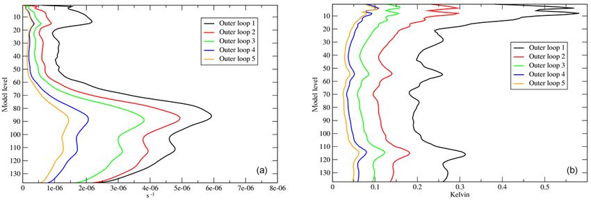
M. Bonavita et al.: Nonlinear effects in 4D-Var                                                                                                721

Figure 7. Vertical profiles of the longitudinally averaged standard deviation of the analysis increments produced at the end of the first outer
loop minimisation (a, c, e) and the fifth outer loop minimisation (b, d, f) for temperature (a, b), vorticity (c, d) and humidity (e, f). Details of
the assimilation experiments as described in text.

   A representative sample of o − a and o − b departures is                 increasing the number of outer loops to four, and to a smaller
shown in Fig. 11. In these plots the observation departures                 extent five, can bring additional benefits in the tropospheric
for a standard three outer loop 4D-Var assimilation cycle are               analysis, in particular for observations sensitive to humid-
used as a baseline against which the departures for one, four               ity and clouds and for wind observations (not shown). This
and five outer loop experiments are compared. The first thing               confirms the diagnostics of Figs. 6 and 7, i.e. that the wind
to note is the significant degradation in both o − a and o − b              and humidity analysis increments in the troposphere are still
statistics of the one outer loop experiment. This degradation               relatively large in the fourth and fifth outer loop updates, in-
is visible for all observation types (not shown) and indicates              dicating that the minimisation has not fully converged.
that a linear analysis update is inadequate in the context of a                The only degradation in o − a and o − b statistics for
12 h assimilation window. The other significant result is that              the four and five outer loop experiments is visible in the

www.nonlin-processes-geophys.net/25/713/2018/                                             Nonlin. Processes Geophys., 25, 713–729, 2018
722                                                                                 M. Bonavita et al.: Nonlinear effects in 4D-Var

Figure 8. (a) Infrared image of the continental US from the GOES-13 geostationary satellite, valid on 3 May 2017, 17:45 UTC (credits:
National Centers for Environmental Information, NOAA). (b) ECMWF operational analysis of geopotential at 200 hPa (continuous isolines),
temperature at 200 hPa (dashed isolines) and equivalent potential temperature at 850 hPa (shaded, units Kelvin), valid on 3 May 2017,
18:00 UTC.

Figure 9. (a) ECMWF operational analysis of geopotential at 200 hPa (continuous isolines), temperature analysis increments at 150 hPa
(colour shaded, units Kelvin) and wind vector analysis increments at 150 hPa (arrows, units m s−1 ), valid on 3 May 2017, 12:00 UTC. (b) as
left, all quantities at 850 hPa.

stratospheric-peaking channels of the microwave (Fig. 11,               rent investigations. Preliminary results indicate that the main
bottom right, channels 10 to 14) and infrared hyperspectral             cause of this behaviour can be traced to the different time
instruments (not shown). This is particularly visible in the            steps used in the inner and outer loops. This difference in
five outer loop experiment, where o − a statistics are clearly          time steps leads to different speeds of propagation of grav-
degraded for channels 10 to 14 (approx. peaking from 50                 ity waves in the stratosphere, which then leads to oscillating
to 2 hPa) while the degradation in the fit to the short-range           behaviour in the minimisation. This is ongoing work and we
forecast (o − b) is only marginal. This result can be partially         defer a more complete treatment of this interesting effect to
explained by the diagnostic shown in Fig. 1, where it was               a future publication.
shown that the magnitude of nonlinear effects in the ECMWF
analysis system is relatively small in the stratosphere. Thus,          5.2   Forecast skill – full observing system
the incremental minimisation can be expected to converge
more rapidly in the stratosphere and additional outer loops
                                                                        The forecast skill scores show a high level of consistency
beyond the standard three cannot be expected to significantly
                                                                        with the analysis skill diagnostics. In Fig. 12 we present a
improve o − a and o − b fits. On the other hand, the reason
                                                                        selection of tropospheric forecast skill scores relevant for
why these fits are actually degraded is the subject of cur-
                                                                        evaluating standard synoptic performance (500 hPa geopo-

Nonlin. Processes Geophys., 25, 713–729, 2018                                     www.nonlin-processes-geophys.net/25/713/2018/
M. Bonavita et al.: Nonlinear effects in 4D-Var 723
Figure 10. Standard deviation of wind vector observation minus model departures over the 09:00 to 21:00 UTC assimilation window of
3 May 2017 in the 100–400 hPa layer for a pre-operational version of the IFS 43R3 cycle: first guess departures (a); a one outer loop analysis
departures (b); a three outer loop analysis departures (c); a five outer loop analysis departures (d).
tential rms forecast error, top row), the water cycle (total col- in the model evolution during the assimilation window and
umn water vapour rms error, second row) and the wind field nonlinearities in the observation operators. It is difficult to
(200 and 850 hPa wind vector rms errors, third and bottom cleanly disentangle the two effects, as they are linked inside
row). All the diagnostics confirm the significant degradation the generalised observation operator G and its linearisations.
in performance for the one outer loop experiment and the We have however tried to evaluate the impact of the model
small but statistically significant improvement of the four and nonlinearities in isolation by running a set of multi-outer loop
five outer loop experiments with respect to the baseline three assimilation experiments where we have retained a subset of
outer loop experiment. In the stratosphere (not shown) fore- observations that are linearly related to the control variables
cast skill scores again show degraded performance for the (conventional in situ observations, atmospheric motion vec-
one outer loop experiment, while results are mostly neutral tors, GPS radio occultation bending angles, microwave tem-
or slightly positive for the four and five outer loop exper- perature sounders). A sample of results from this set of ex-
iments. One notable exception is the tropical stratospheric periments is presented in Fig. 13, which shows the same set
layer from 5 to 1 hPa, where the five outer loop experiment of forecast skill scores shown in Fig. 12 for the experiments
shows a statistically significant degradation, again confirm- with the full observing system. It can be seen that the impact
ing the analysis skill diagnostic results. of going from one to three outer loops is still very signifi-
cant. However, the impact of going from three to four outer
5.3 Analysis and forecast skill – linear observation loops appears to be smaller than in the experiments with the
operators full observing system, and this effect is visible in other fore-
cast skill measures as well (not shown). This suggests that in
the current ECMWF 4D-Var it is the presence of nonlinear
In Sect. 2 of this paper we have shown how nonlinear effects
observations (in particular the all-sky radiances sensitive to
in 4D-Var arise from two different sources: nonlinearities
www.nonlin-processes-geophys.net/25/713/2018/ Nonlin. Processes Geophys., 25, 713–729, 2018724 M. Bonavita et al.: Nonlinear effects in 4D-Var
Figure 11. Normalised standard deviations of analysis (o − a) and first guess (o − b) departures for radiosonde temperature observations (a);
radiosonde humidity observations (b); the microwave imager AMSR-2 (c); the combined observations from the AMSU-A microwave sounder
instrument onboard the AQUA, METOP-A/B, and NOAA-15/18/19 satellites (d). The 100 % baseline refers to the three outer loop ex-
periment, the black/red/green lines to the one/four/five outer loop experiments, respectively. Values smaller/larger than 100 indicated a
tighter/looser fit of the analysis/first guess to the observations relative to the three outer loop baseline experiment. Values are averaged over
the 20 December 2016 to 28 February 2017 period. Error bars represent 95 % confidence levels.
cloud and precipitation) that is responsible for the additional pacity of the assimilation algorithms to deal effectively with
benefit of running more than the current three outer loops. nonlinear effects an increasingly important benchmark.
The ECMWF implementation of 4D-Var relies on a pertur-
bative approach to nonlinearity. Incremental 4D-Var is based
on the concept of a purely linear analysis update iterated
6 Discussion and conclusions on ever more accurate first guess trajectories. Diagnostics in
both observation space and model space support this inter-
In modern atmospheric data assimilation (and, arguably, in pretation and show that the capacity to run more than one
most of the other Earth system components as well) nonlin- outer loop is a significant driver of the overall ECMWF anal-
earities play an ever more important role. This is due to the ysis and forecast skill. Results from long data assimilation
ever-increasing resolution and complexity of the prognostic cycling experiments show that running the current ECMWF
models, which exhibit instabilities at smaller scales and thus 4D-Var with one outer loop only, which is equivalent to mak-
present faster nonlinear error growth during the assimilation ing a purely linear analysis update, would result in very sig-
window, and to the emergence of an array of observations nificant deterioration in all analysis and forecast accuracy
that are nonlinearly related to the control vector variables metrics. Conversely, adding one, or possibly two additional
used in the variational analyses. Both these trends are ex- outer loops to the current operational set-up of three outer
pected to continue in the near future, which makes the ca-
Nonlin. Processes Geophys., 25, 713–729, 2018 www.nonlin-processes-geophys.net/25/713/2018/M. Bonavita et al.: Nonlinear effects in 4D-Var 725 Figure 12. Normalised root mean square forecast errors for geopotential at 500 hPa (a); total column water vapour (b); wind vector at 200 hPa (c); wind vector at 850 hPa (d). The black/red/green lines refer to the one/four/five outer loop experiments, respectively. Errors are normalised with respect to the three outer loop experiments and are computed using the operational ECMWF analysis as verification. Error bars represent 95 % confidence levels. loop updates, appear beneficial both in terms of analysis assimilation system. As noted in Sect. 5, while the tropo- quality and in terms of general forecast skill. Results from spheric analyses and forecasts were consistently improved in limited additional experimentation (not shown) also indicate the four and five outer loop assimilation experiments, signs that more than five outer loops do not appear to bring further of degradation started to appear in the analysis and first guess benefits, at least in the experimental configuration we have fit of some types of stratospheric peaking radiance observa- used. tions. Interestingly, these degradations were not seen in the One interesting question is about the limits of applicabil- experiments using only observations which are linearly re- ity of the multi-incremental approach in the ECMWF data lated to the state. This suggests that changes to the analy- www.nonlin-processes-geophys.net/25/713/2018/ Nonlin. Processes Geophys., 25, 713–729, 2018
726                                                                                   M. Bonavita et al.: Nonlinear effects in 4D-Var

Figure 13. Normalised root mean square forecast errors for geopotential at 500 hPa (a); total column water vapour (b); wind vector at
200 hPa (c); wind vector at 850 hPa (d) for the assimilation experiments using the linear observations subset. The black/red lines refer to the
one/four outer loop experiments, respectively. Errors are normalised with respect to the three outer loop experiment and are computed using
the operational ECMWF analysis as verification. Error bars represent 95 % confidence levels.

sis introduced by the assimilation of nonlinear observations              the hypothesis that the representation in the 4D-Var analysis
(mainly humidity and cloud and precipitation sensitive ra-                of stratospheric gravity waves excited by the assimilation of
diances) affect the stratospheric analysis either through the             all-sky observations could be one of the main drivers of these
shape of the background error spatial correlations or by the              effects. These interactions are currently being investigated.
generation of gravity wave structures in the initial conditions.             Another obvious factor potentially limiting the applica-
Remarkably, the stratospheric degradation of the multi-outer              bility of the incremental algorithm is the range of validity
loop experiments also disappeared in tests run with the full              of the tangent linear (TL) hypothesis (Sect. 2). As reported
observing system with matching time steps for the outer and               in Bonavita et al. (2017b), problems in 4D-Var convergence
inner loop integrations. This result gives further support to             connected with the TL hypothesis usually arise in situations

Nonlin. Processes Geophys., 25, 713–729, 2018                                        www.nonlin-processes-geophys.net/25/713/2018/
M. Bonavita et al.: Nonlinear effects in 4D-Var                                                                                      727

where the first guess departures are at least 1 order of mag-        Competing interests. The authors declare that they have no conflict
nitude larger than the assumed observation errors. In most           of interest.
cases, use of more realistic values of the observation errors,
which better take into account the representativity and obser-
vation operator components, are sufficient to regularise the         Special issue statement. This article is part of the special is-
minimisation.                                                        sue “Numerical modeling, predictability and data assimilation in
   While the advantages of being able to run an increased            weather, ocean and climate: A special issue honoring the legacy of
                                                                     Anna Trevisan (1946–2016)”. It is a result of a Symposium Honor-
number of outer loop linearisations are clear, the question
                                                                     ing the Legacy of Anna Trevisan – Bologna, Italy, 17–20 October
remains on how to fit them inside the typically tight opera-
                                                                     2017.
tional schedules of operational weather centres. Taking the
ECMWF data assimilation system as an example, the three
outer loops 4D-Var analysis has about 45 min to complete.            Acknowledgements. One of the authors (Massimo Bonavita) would
Given the sequential nature of the 4D-Var minimisation, each         like to express his gratitude to the organisers of the Anna Trevisan
additional outer loop would increase this time by approx.            Symposium, and to Alberto Carrassi in particular, for setting up a
15 min. This implies that, in the current set-up, the obser-         very successful and interesting meeting and for being such attentive
vation cut-off time would have to be pushed back by a simi-          and considerate hosts.
lar time interval, quickly negating any advantage that the in-          The authors would also like to thank the reviewers and the
creased number of outer loops might bring. One possible way          editor for their careful examination of our manuscript and the many
to overcome this problem would be to allow late arriving ob-         constructive proposals for its improvement.
servations to enter the assimilation at successive outer loop
                                                                     Edited by: Michael Ghil
updates. This would effectively push the observation cut-off
                                                                     Reviewed by: four anonymous referees
time forward to the beginning of the last minimisation, thus
allowing to start the 4D-Var analysis earlier and consequently
accommodate additional outer loop updates. This assimila-
tion framework, which we call “continuous DA”, is currently          References
being tested at ECMWF and results will be documented in a
                                                                     Andersson, E., Fisher, M., Holm, E., Isaksen, L., Radnòti,
forthcoming paper. Note that in the continuous DA the prob-
                                                                       G., and Trémolet, Y.: Will the 4D-Var approach be de-
lem being solved is conceptually different from that of incre-
                                                                       feated by nonlinearity? ECMWF Tech. Memo. 479, avail-
mental 4D-Var. In incremental 4D-Var we solve a nonlinear              able at: https://www.ecmwf.int/sites/default/files/elibrary/2005/
problem through repeated linearisations. In the continuous             7768-will-4d-var-approach-be-defeated-nonlinearity (last ac-
DA we solve a sequence of slightly different nonlinear min-            cess: 1 September 2018), 2005.
imisation problems, taking advantage of increasingly accu-           Bauer, P., Geer, A. J., Lopez, P., and Salmond, D.: Direct 4D-Var as-
rate first guess trajectories.                                         similation of all-sky radiances. Part I: Implementation, Q. J. Roy.
   Another possible approach to increase the number of outer           Meteor. Soc., 136, 1868–1885. https://doi.org/10.1002/qj.659,
loops within the operational time constraints is to adopt an           2010.
“overlapping” assimilation window framework, for exam-               Björck, A.: Numerical methods for least squares problems, SIAM,
ple along the lines discussed in Bonavita et al. (2017a). In           Philadelphia, ISBN 0-89871-360-9, 1996.
                                                                     Bonavita, M., Trémolet, Y., Holm, E., Lang, S. T. K., Chrust, M.,
this configuration, observations that have been assimilated in
                                                                       Janisková, M., Lopez, P., Laloyaux, P., De Rosnay, P., Fisher, M.,
both successive overlapping windows will have effectively
                                                                       Hamrud, M., and English, S.: A Strategy for Data Assimilation,
be seen by twice the number of guess trajectories as in a stan-        ECMWF Technical Memorandum n. 800, available at: https:
dard non-overlapping configuration. This idea, similar to the          //www.ecmwf.int/en/elibrary/17179-strategy-data-assimilation
quasi-static variational DA approach of Pires et al. (1996)            (last access: 1 September 2018), 2017a.
and Jarvinen et al. (1996), is also being actively investigated.     Bonavita, M., Dahoui, M., Lopez, P., Prates, F., Hólm, E., De
                                                                       Chiara, G., Geer, A., Isaksen, L., and Ingleby, B.: On the ini-
                                                                       tialization of Tropical Cyclones. ECMWF Technical Memo-
Data availability. The datasets used in this work are avail-           randum n. 810, available at https://www.ecmwf.int/en/elibrary/
able from ECMWF under the terms and conditions specified               17677-initialization-tropical-cyclones (last access: 1 Septem-
at         https://www.ecmwf.int/en/forecasts/accessing-forecasts/     ber 2018), 2017b.
order-historical-datasets (last access: 1 September 2018).           Carrassi, A., Ghil, M., Trevisan, A., and Uboldi, F.: Data assim-
                                                                       ilation as a nonlinear dynamical system problem: Stability and
                                                                       convergence of the prediction-assimilation system, Chaos, 18,
Author contributions. All the authors have equally contributed to      023112, https://doi.org/10.1063/1.2909862, 2008.
all parts of the paper and the work described in it.                 Courtier, P., Thépaut, J.-N., and Hollingsworth, A.: A strategy
                                                                       for operational implementation of 4D-Var, using an incre-
                                                                       mental approach, Q. J. Roy. Meteor. Soc., 120, 1367–1387,
                                                                       https://doi.org/10.1002/qj.49712051912, 1994.

www.nonlin-processes-geophys.net/25/713/2018/                                    Nonlin. Processes Geophys., 25, 713–729, 2018
728 M. Bonavita et al.: Nonlinear effects in 4D-Var Fisher, M.: Minimization Algorithms for Variational Data search Activities in Atmospheric and Oceanic Modelling, 34, 1– Assimilation. Proceedings of the ECMWF Seminar on Re- 17, 2005. cent Developments in Numerical Methods for Atmospheric Laroche, S. and Gauthier, P.: A validation of the incre- Modelling, available at: https://www.ecmwf.int/en/elibrary/ mental formulation of 4D variational data assimilation 9400-minimization-algorithms-variational-data-assimilation in a nonlinear barotropic flow, Tellus A, 50, 557–572, (last access: 1 September 2018), 1998. https://doi.org/10.3402/tellusa.v50i5.14558, 1998. Fisher, M.: Estimation of entropy reduction and degrees of Lawless, A. S., Gratton, S., and Nichols, N. K.: Approximate it- freedom for signal for large variational analysis systems, erative methods for variational data assimilation, Int. J. Numer. ECMWF Technical Memorandum n. 397, available at: Meth. Fl., 47, 1129–1135, https://doi.org/10.1002/fld.851, 2005. https://www.ecmwf.int/en/elibrary/9402-estimation-entropy- Lorenc, A. C. and Payne, T.: 4D-Var and the butterfly ef- reduction-and-degrees-freedom-signal-large-variational- fect: Statistical four-dimensional data assimilation for a wide analysis (last access: 1 September 2018), 2003. range of scales, Q. J. Roy. Meteor. Soc., 133, 607–614, Gauthier, P.: Chaos and quadri-dimensional data assimilation: https://doi.org/10.1002/qj.36, 2007. a study based on the Lorenz model, Tellus A, 44, 2–17, Maddox, R. A.: Mesoscale Convective Complexes, B. Am. https://doi.org/10.1034/j.1600-0870.1992.00002.x, 1992. Meteorol. Soc., 61, 1374–1387, https://doi.org/10.1175/1520- Gauthier, P., Tanguay, M., Laroche, S., Pellerin, S., and Morneau, J.: 0477(1980)0612.0.CO;2, 1980. Extension of 3DVAR to 4DVAR: implementation of 4DVAR at Malardel, S., Wedi, N., Deconinck, W., Diamantakis, M., Kühn- the meteorological service of Canada, Mon. Weather Rev., 135, lein, C., Mozdzynsky, G., Hamrud, M., and Smolarkiewicz, P.: 2339–2354, https://doi.org/10.1175/MWR3394.1, 2007. A new grid for the IFS. ECMWF Newsletter No. 146, Winter Geer, A. J. and Bauer, P.: Observation errors in all-sky 2015/16, available at: https://www.ecmwf.int/sites/default/files/ data assimilation, Q. J. R. Meteor. Soc., 137, 2024–2037, elibrary/2016/17262-new-grid-ifs.pdf (last access: 1 Septem- https://doi.org/10.1002/qj.830, 2011. ber 2018), 2016. Geer, A. J., Baordo, F., Bormann, N., Chambon, P., English, S. J., Miller, R. N., Ghil, M., and Gauthiez, F.: Advanced Data Kazumori, M., Lawrence, H., Lean, P., Lonitz, K., and Lupu, C.: Assimilation in Strongly Nonlinear Dynamical Systems, J. The growing impact of satellite observations sensitive to humid- Atmos. Sci., 51, 1037–1056, https://doi.org/10.1175/1520- ity, cloud and precipitation, Q. J. Roy. Meteor. Soc., 143, 3189– 0469(1994)0512.0.CO;2, 1994. 3206, https://doi.org/10.1002/qj.3172, 2017. Pires, C., Vautard, R., and Talagrand, O.: On extending the limits of Gratton, S., Lawless, A., and Nichols, N. K.: Approximate Gauss– variational assimilation in nonlinear chaotic systems, Tellus A, Newton methods for nonlinear least squares problems, SIAM 48, 96–121, 1996. J. Optimiz., 18, 106–132, https://doi.org/10.1137/050624935, Rabier, F. and Courtier, P.: Four-Dimensional Assimilation in the 2007. Presence of Baroclinic Instability, Q. J. Roy. Meteor. Soc., 118, Hólm, E. V., Andersson, E., Beljaars, A. C. M., Lopez, P., 649–672, https://doi.org/10.1002/qj.49711850604, 1992. Mahfouf, J.-F., Simmons, A., and Thépaut, J.-J.: Assimila- Rabier, F., Järvinen, H., Klinker, E., Mahfouf, J.-F., and Sim- tion and Modelling of the Hydrological Cycle: ECMWF’s mons, A.: The ECMWF operational implementation of four- Status and Plans. ECMWF Tech. Memo. 383, available at: dimensional variational assimilation. Part I: Experimental results https://www.ecmwf.int/sites/default/files/elibrary/2002/9996- with simplified physics, Q. J. Roy. Meteor. Soc., 126, 1143– assimilation-and-modelling-hydrological-cycle-ecmwfs-status- 1170, https://doi.org/10.1002/qj.49712656415, 2000. and-plans.pdf (last access: 1 September 2018), 2002. Radnòti, G., Trémolet, Y., Andersson, E., Isaksen, L., Hólm, Hoteit, I.: A reduced-order simulated annealing approach for E. V., and Janiskova, M.: Diagnostics of linear and in- four-dimensional variational data assimilation in meteorology cremental approximations in 4D-Var revisited for higher and oceanography, Int. J. Numer. Meth. Fl., 58, 1181–1199, resolution analysis, ECMWF Tech Memo 479, available at: https://doi.org/10.1002/fld.1794, 2008. https://www.ecmwf.int/en/elibrary/11816-diagnostics-linear- Isaksen, L., Bonavita, M., Buizza, R., Fisher, M., Haseler, and-incremental-approximations-4d-var-revisited-higher (last J., Leutbecher, M., and Raynaud, L.: Ensemble of access: 1 September 2018), 2005. data assimilations at ECMWF. ECMWF Tech. Memo. Rawlins, F., Ballard, S. P., Bovis, K. J., Clayton, A. M., Li, 636, available at: https://www.ecmwf.int/en/elibrary/ D., Inverarity, G. W., Lorenc, A. C., and Payne, T. J.: 10125-ensemble-data-assimilations-ecmwf (last access: The Met Office global four-dimensional variational data as- 1 September 2018), 2010. similation scheme, Q. J. Roy. Meteor. Soc., 133, 347–362, Janisková, M. and Lopez, P.: Linearized physics for data assimila- https://doi.org/10.1002/qj.32, 2007. tion at ECMWF, in: Data assimilation for Atmospheric, Oceanic Rodwell, M. J., Magnusson, L., Bauer, P., Bechtold, P., Bonavita, and Hydrological Applications (Vol. II), edited by: Park, S. M., Cardinali, C., and Diamantakis, M.: Characteristics of occa- K. and Xu, L., Springer-Verlag Berlin Heidelberg, 251–286, sional poor medium-range weather forecasts for Europe, B. Am. https://doi.org/10.1007/978-3-642-35088-7, 2013. Meteorol. Soc., 94, 1393–1405, https://doi.org/10.1175/BAMS- Jarvinen, H., Thépaut, J. N., and Courtier, P.: Quasi-continuous vari- D-12-00099.1, 2013. ational data assimilation, Q. J. Roy. Meteor. Soc., 122, 515–534, Rosmond, T. and Xu, L.: Development of NAVDAS-AR: non- 1996. linear formulation and outer loop tests, Tellus A., 58, 45–58, Kadowaki, T.: A 4-Dimensional Variational Assimilation System https://doi.org/10.1111/j.1600-0870.2006.00148.x, 2006. for the JMA Global Spectrum Model, CAS/JAC WGNE Re- Nonlin. Processes Geophys., 25, 713–729, 2018 www.nonlin-processes-geophys.net/25/713/2018/
You can also read