Challenges of Numerical Simulation of Dynamic Wetting Phenomena: A Review
←
→
Page content transcription
If your browser does not render page correctly, please read the page content below
Challenges of Numerical Simulation of
                                                               Dynamic Wetting Phenomena: A Review

                                                                                     Shahriar Afkhami
arXiv:2108.05994v1 [physics.flu-dyn] 12 Aug 2021

                                                    Department of Mathematical Sciences, New Jersey Institute of Technology, Newark, NJ,
                                                                                        USA 07102

                                                   Abstract
                                                   Wetting is fundamental to many technological applications that involve the mo-
                                                   tion of the fluid-fluid interface on a solid. While static wetting is well understood
                                                   in the context of thermodynamic equilibrium, dynamic wetting is more compli-
                                                   cated in that liquid interactions with a solid phase, possibly on molecular scales,
                                                   can strongly influence the macroscopic scale dynamics. The problem with con-
                                                   tinuum models of wetting phenomena is then that they ought to be augmented
                                                   with microscopic models to describe the molecular neighborhood of the moving
                                                   contact line. In this review, widely used models for the computation of wetting
                                                   flows are summarized first, followed by an overview of direct numerical simu-
                                                   lations based on the Volume-of-Fluid approach. Recent developments in the
                                                   Volume-of-Fluid simulations of the wetting are then reviewed, with a particular
                                                   attention paid on combining macro-scale simulations with the hydrodynamic
                                                   theory near the moving contact line, as well as including a microscopic descrip-
                                                   tion by coupling with the van der Waals interface model. Finally, the extension
                                                   to modeling the contact line motion on non-flat surfaces is surveyed, followed
                                                   by hot topics in nucleate boiling.
                                                   Keywords:

                                                   1. Introduction

                                                       Wetting phenomena involves the motion of the interface between two or more
                                                   fluids in contact with a solid [1]. Many natural and industrial processes are inti-
                                                   mately related to the details of wetting phenomena. As technological capability
                                                   evolves, it becomes increasingly important to understand the fundamentals of
                                                   the fluid dynamical interactions involved in such applications, in order to opti-
                                                   mize system performance. Numerical modeling offers great potential to predict
                                                   outcomes under given conditions, and hence, ultimately, to optimize the pro-
                                                   cess. Moreover, computational tools can play a very important role in terms of

                                                     ∗ Correspondingauthor
                                                      Email address: shahriar.afkhami@njit.edu (Shahriar Afkhami)

                                                   Preprint submitted to Journal of LATEX Templates                       August 16, 2021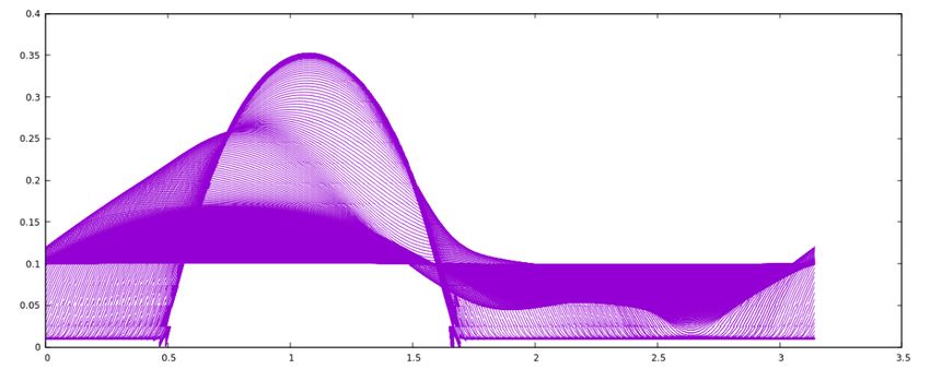
enhancing our understanding of the physics involved, and allowing predictions
to be made cheaply.
    Simulating wetting phenomena is complicated due to the presence of moving
‘contact lines’ (the lines at which a fluid-fluid interface meets a solid surface)
[2–6]. Considerable research effort has been directed to study such problem;
see e.g. [7, 8] for a comprehensive (and relatively recent) reviews. Simulating
such phenomena is further complicated, in part, by the fact that the description
of moving contact lines involves widely varying characteristic lengths [9–12],
from macroscopic to near molecular length scales. The motion of the fluid near
the contact line and the dynamic behavior of the interface itself present fur-
ther complications, and analytical solutions exist only for very simple problems.
Numerical simulations can yield accurate predictions but have been far less
successful when studying wetting phenomena. For such problems, the efficacy
of numerical simulation is highly dependent on the ability of accurately and
robustly computing the moving contact line.
    Another potential issue is that at the contact line, as the characteristic length
of the problem becomes smaller and the surface tension starts to dominate
over other forces, the surface tension discretization becomes a key ingredient
in the feasible computation of such flows. For these reasons, though reliable
codes exist for the simpler two dimensional problem, there are relatively few
examples of three dimensional codes that incorporate algorithms for treating
dynamic contact lines; [13–19] are representative of the variety of approaches
that are used. Moreover, robust and accurate numerical models are needed for
simulating fluid-structure interactions that involve moving solid objects in an
interfacial flow that also includes contact lines (see e.g. [18, 20]).
    While there exist different numerical approaches which can deal with dy-
namic contact lines, here we concentrate on the ‘Volume-of-Fluid’ (VOF) method,
with our main goal to be to represent recent developments for the implemen-
tation of the contact angle boundary condition at a moving contact line, self-
consistent numerical validations, a dynamic contact angle model based on a
hydrodynamic description of the contact line, as well as an approach for the
direct inclusion of liquid-solid interaction. We specifically pursue Gerris [21]
numerical framework to describe the implementations of the methods. The
interested reader is referred to the works in [22–24] for further details and dis-
cussions. However, we also note possibilities of using other tools than Gerris,
such as the use of its successor code Basilisk [25]; see e.g. [19, 26, 27] for very
recent studies that utilize Basilisk for the numerical simulation of dynamic con-
tact line. While the focus of this review is on a VOF method, we note that
a major challenge for the simulation of moving contact lines in all continuum
based approaches is to obtain mesh-independent results with no adjustable pa-
rameters. The development of such models will require resolving all the length
scales, typically from nanoscale at the solid boundary to bulk sizes, which can
be of a millimeter size or more. For feasible computations therefore sub-grid
models ought to be introduced, and as a result, the key ingredient in all current
and previous models is to bridge the macroscale dynamics to the characteristics
of the contact line at the nanoscale.

                                         2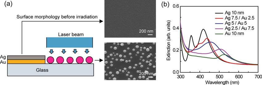
The nature of flows in a neighborhood of a moving contact line and the
matching of local solutions to the global flow have been the topic of a number
of investigations; see e.g. [28, 29]. Despite the huge research effort, however,
a full understanding of the mechanism by which a contact line moves along a
solid surface is still incomplete. While numerical investigations can enhance our
understanding of the physics involved, simulating dynamic contact line flows
is complicated by the mathematical paradox of a contact line moving along a
no-slip solid surface, first discussed by Huh and Scriven in [30]. Here we will
review major difficulties involved in continuum-level numerical simulations in
the VOF numerical framework, mainly: (i) how to specify the dynamic contact
angle; and (ii) how to modify the no-slip boundary condition to remove the
stress singularity [6, 31].
    We first give a concise account of a variety of other computational meth-
ods that have been considered in the context of wetting phenomena. Here we
mention level set methods that use a continuous function to describe the inter-
face. A reconstruction of the continuous function in the ghost domain is used
to impose the contact angle within the level set approach [3, 32, 33]. (The
grid points across the boundary are treated as ghost points). We also men-
tion phase-field methods that treat two fluids with a diffuse interface by means
of a smooth concentration function, which typically satisfies the Cahn-Hilliard
or Allen–Cahn equations [34], and is coupled to the Navier–Stokes equations.
Jacqmin [35] describes a phase-field contact angle model that uses a wall energy
to determine the value of the normal derivative of the concentration on a solid
substrate. This model has been used to study contact line dynamics [2, 36], and
similar models have been considered in the investigation of the sharp interface
limit of the diffuse interface model [37, 38]. Lattice-Boltzmann methods have
also treated the contact angle with a wall energy contribution [39, 40]. Molec-
ular dynamics (MD) simulations [41–44] have also been considered, where the
interaction between fluid and solid particles is described by the Lennard–Jones
potential, albeit mainly for simulating nanoscale systems.
    In [45], the authors carry out continuum based computations of dewetting
of molten nanoparticles on a solid and show quantitative agreement with MD
simulations, when either using a free-slip boundary condition, or a partial slip
with a slip length of nanometer sizes. In [46], the authors carry out simulations
of steady water drop sheared between two moving plates using MD, phase-
field, and VOF methods. They show discrepancy, when comparing the results
from phase-field to MD simulations. Moreover, they show that with a suitable
choice of parameters and boundary conditions in the phase-field simulations,
a reasonable agreement with MD can be obtained. They also reproduce the
MD results reasonably well with the VOF simulations using a localized slip
boundary condition. Interestingly, they point out the role of diffusion in their
phase-field model and the physical interpretation of it, showing different effect
to what happens in MD simulations, suggesting a perfect agreement cannot be
expected. In summary, the authors in [46] point out the necessity for hybrid
methods for matching MD with continuum solvers, similar in spirit to that in
[47].

                                       3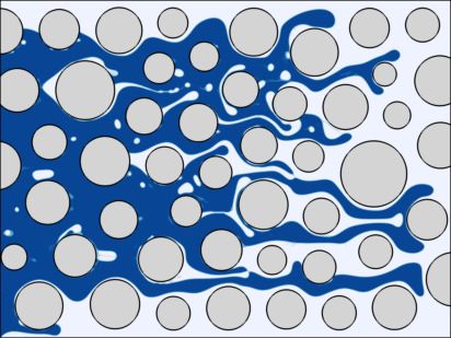
Finally, in the context of front-tracking methods, in [48], the authors im-
plement a front-tracking method and use a partial slip boundary condition and
an ad hoc model for the determination of the dynamic contact angle based on
the contact line speed. Recently, in [16], the authors developed a front-tracking
approach for simulating dynamic contact angles, where the contact line motion
is described by a slip model.
    In what follows, we first present in Sec. 2, a multiscale wetting/dewetting
model based on an adaptive VOF method coupled with van der Waals interac-
tion, which can be considered as a mesoscopic approach to model liquid-solid
interaction. We then review a work on wetting transitions in Sec. 3. In Sec. 4,
we discuss an approach to model the contact line motion on non-flat surfaces
and its application to simulating a two-phase flow in porous media. Lastly, in
Sec. 5, as an example of a future direction, we present nucleate boiling, where
resolving the details of the flow around a moving contact line is of a significant
importance to building a generally applicable numerical model.

2. A mesoscopic approach to model liquid-solid interaction

    It is impossible for a contact line to move on a solid if a molecularly sharp
fluid-fluid interface is considered along with a strictly no-slip solid. The conse-
quence of such is the divergence of shear stress upon approaching the contact
line. As elegantly stated by Pomeau in [10], “One major difficulty met when
trying to ‘solve’ the moving contact line problem is to find at which scale the
usual continuum mechanics breaks down and should be amended to get rid of
the divergence.”. Here, we review a recently developed computational scheme
for wetting/dewetting flows, that combines the van der Waals model with the
Navier-Stokes equations to devise a divergence free numerical framework for the
simulation of contact line motion [49]. We show how this approach can lead to
accurate description of the contact line, while recovering the usual macroscopic
scale flow far away from the contact line.
    Let us begin by considering the incompressible Navier–Stokes equations for a
two-phase flow. We refer to two phases as the liquid phase (subscript l), and the
vapor phase (subscript v), i.e. i = l, v, with no loss of generality. We introduce a
characteristic function χ(x, y, z, t), which takes the value of 1 inside of the liquid
phase, and 0 inside the vapor phase. The interface between these two phases is
assumed to be sharp, so that χ changes discontinuously at the interface. The
governing equations then are
                Du
                   = −∇p + ∇ · µ(χ) ∇u + ∇u> + γκnδs + FvdW ,

         ρ(χ)                                                                     (1)
                Dt

                                     ∇ · u = 0.                                   (2)
Here, ρ(χ) = ρl χ + ρv (1 − χ) is the density, µ(χ) = µl χ + µv (1 − χ) the viscosity,
p the pressure, and u the velocity vector. Also

                           Dχ/Dt = ∂t χ + u · ∇χ = 0.                             (3)

                                          4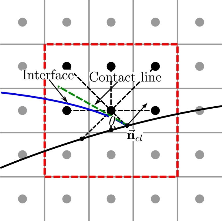
Figure 1: A schematic of the fluid-fluid-solid interactions.

The surface tension is included as a singular body force (per unit volume) [24,
50], where γ is the surface tension coefficient, κ the interfacial curvature, δs a
delta function centered on the interface, and n a normal vector for the interface
pointing out of the liquid. The total body force due to the van der Waals
interaction is represented by FvdW , which we describe next.
    We consider a solid phase occupying a half-infinite region y < 0, above
which there is a region occupied by two fluids, see Fig. 1. Each particle of fluid
phase i interacts with the solid substrate by means of a Lennard–Jones type
potential [11, 12]
                                        σ a  σ b
                          φis = Kis          −         ,                       (4)
                                        r        r
where r is the distance between the two particles, and Kis is the scale of the
potential. The total potential energy in phase i due to this interaction is
                                 m  n
                                  h         h
                  Φis (y) = Kis         −         = Kis ψ(y),               (5)
                                  y         y

where                                                                      1
                                                                        ! a−b
                                                                  b−3
                                               [(a − 2)(a − 3)]
                 Kis = 2πni ns Kis σ 3                         a−3              ,    (6)
                                               [(b − 2)(b − 3)]
                                         1
                     (a − 2)(a − 3)
                                      a−b
            h=                                σ;       m = a − 3,       n = b − 3,   (7)
                     (b − 2)(b − 3)
where ni and ns are the densities of particles in fluid phase i and the solid
substrate, respectively. Equation 5 gives the total potential per unit volume in
fluid phase i due to the interaction with the solid substrate. The quantity h
is conventionally referred to as the equilibrium film thickness in the literature.
The parameters m and n are taken based on the choices of a and b in Eq. 4; see
[49, 51], for example.
    The force per unit volume on phase i as a results of the potential, Eq. 5, is
Fis (y) = −∇Φis (y), where

                             FvdW = χF̂ls + (1 − χ)F̂vs ,                            (8)

                                                   5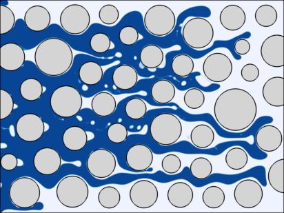
0.25
           0.20
           0.15
           0.10
           0.05
           0.00
               0.0 0.2 0.4 0.6 0.8 1.0 1.2 1.4
Figure 2: Equilibrium profiles (solid lines) for θi = θeq = π/4; the arrow shows the direction
of decreasing h. The dotted lines show the initial profile. h = 0.025(blue), 0.0125(green),
0.00625(black);

It can then be shown [49] that

                                    (1 − cos θeq ) (m − 1)(n − 1)
             FvdW = ∇pvdW +                                       ψ(y)nδs .               (9)
                                          h            m−n
The first term on the right hand side of Eq. 9 is absorbed into the pressure
gradient in Eq. 1 for the entire domain, while the second term is centered only
on the interface. We refer the interested readers to [24] for the details of the
discretization of κ in Eq. 1, and n and δs , in Eqs. 1 and 9.
     The coefficient in the second term on the right hand side of Eq. 9 involving
the equilibrium contact angle θeq can be derived based on simple energetic
arguments (see [49]). In this context, there is an equilibrium film of thickness
h that wets the entire substrate, with a smooth transition from the interface
away from the contact to the film. The contact angle can then be defined by
finding the slope of the interface at the transition region. For example, for a
drop at equilibrium with a vanishingly small h, we measure contact angles by
fitting a circular profile to the droplet profile ‘away’ from the transition region;
the angle at which this circular profile intersects with the equilibrium film is
taken to be the contact angle, θeq . For non-vanishing but small h, a drop at
equilibrium will have a (slightly) different contact angle, which we refer to as
θnum . Figure 2 shows how the simulated equilibrium contact angle, θnum , is
generally smaller than the imposed angle θeq . This is due to the fact that Eq. 9
is derived under the assumption of small h. Figure 2 also shows the results
when h is varied from 0.025 to 0.00625. The initial condition is imposed with
θi = π/4. As shown, the initial drops, depicted by the black (dotted) profiles,
relax to the equilibrium profiles, and as h is decreased, the equilibrium profiles
are characterized by contact angles closer to prescribed by θeq .

                                              6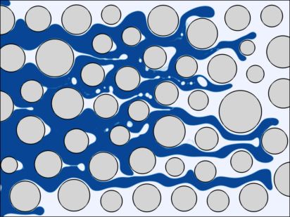
0.40                                                  0.40
       0.35                                                  0.35
       0.30                                                  0.30
       0.25                                                  0.25
       0.20                                                  0.20
       0.15                                                  0.15
       0.10                                                  0.10
       0.05                                                  0.05
       0.00                                                  0.00
           0.0 0.2 0.4 0.6 0.8 1.0 1.2 1.4                       0.0 0.2 0.4 0.6 0.8 1.0 1.2 1.4

                       (a)                                                   (b)

             100                                                   101

                                                                   100
         10−1
  θ3 − θeq

                                                        θ3 − θeq
        3

                                                              3
                                                               10−1
              −2
         10
                                                               10−2

         10−3 −3                                               10−3 −3
            10            10−2               10−1                 10            10−2               10−1
                             vf                                                    vf

                       (c)                                                   (d)

Figure 3: (a) Spreading of drop from initial contact angle θi = π/3 to equilibrium defined by
θeq = π/6 and (b) retraction from θi = π/6 to θeq = π/3. Comparison with the Cox-Voinov
law for (c) spreading and (d) retracting drop. The blue (symbols) shows simulation results and
the black (dashed) line is proportional to vf , showing the expected slope if the Cox-Voinov
[52, 53] law is obeyed.

2.1. Results
     We present the results of droplets with the contact angles imposed by means
of the discretization of Eq. 9 as described in [49, 51]. The initial simulation
setup is a drop on an equilibrium film, initially at rest, which then relaxes to
equilibrium under the influence of the van der Waals force. For all the results
shown next, ρl,v = µl,v = γ = 1, h = 0.025, and (m, n) = (3, 2). Figures 3(a-b)
show the results of droplet spreading and retracting. As shown, the droplet
spreads/retracts to its equilibrium configuration, defined by the θeq . We also
compare the qualitative behavior of the spreading/retracting drop to the well
known Cox-Voinov law [53]. For a drop displacing another immiscible fluid on
a solid surface, the speed of the contact point, vf , is related to instantaneous
angle θ and the equilibrium contact angle θeq to the leading order by θ3 − θeq 3
                                                                                 ∝
vf [52]. As shown, the drop spreading/retracting follows the Cox-Voinov law
for vf ∈ (10−2 , 10−1 ).
     Finally, we mention the dewetting phenomena of liquid films: for a suf-
ficiently thin liquid layer (or multi-layers) on a solid substrate, destabilizing
effects, such as long range fluid-solid interactions, can lead to the film breakup

                                                    7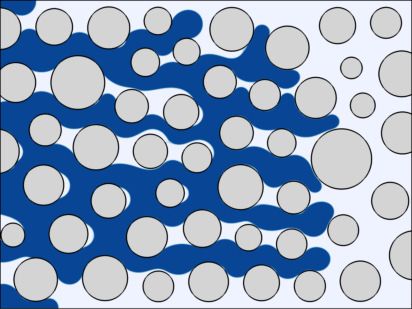
Figure 4: From [58]. (a) Morphologies of a bilayer thin film before and after laser irradiation.
(b) Extinction spectra measured after thins films of different layer combination are dewetted.
and the consequent dewetting phenomena (exposure of prewetted/nominally
dry patches), known as ‘spinodal dewetting’ [54]. Therefore, it is necessary to
include a destabilizing mechanism, such as the van der Waals interactions as de-
scribed above, or otherwise a continuous film does not breakup. While studying
the dewetting of a thin film is commonplace, see e.g. [55–57], there is less effort
in direct numerical simulations of multi-layer dewetting, and the understanding
of competing forces for such systems is currently poor. Below, we describe our
recent results of the dewetting of miscible liquid two-layers on substrates. In
particular, we mention the work in [58] on the fabrication of Ag–Au bimetallic
nanoparticles by laser-induced dewetting of bilayer films; see for example, Fig. 4.
Next we show examples of direct numerical simulations to study the structural
evolution and morphology of bilayer thin films consisted of miscible liquids. We
will concentrate in particular on the role of the contact angle and the viscosity
ratio of the two layers to study how changing these properties may affect the
profile of the fluid as it dewets. We keep the geometrical features fixed, and set
the density ratio and surface tension to 1, with a negligibly small surrounding
viscosity. Figure 5 depicts the schematic of the computational setup. We then
vary the contact angle and the liquid two-layer viscosity ratio and consider two
main scenarios where the breakup of the film results in either an unchanged
length scale, namely leading to the formation of one drop, or ‘dry spots’, lead-
ing subsequently to the formation of one main drop and a secondary droplet.
The findings here will help to understand how to control the synthesis of alloy
metallic nanoparticles, see e.g. [59]. Basilisk [25], which is the Gerris successor
numerical framework, is used here. We have specifically found: 1) In the absence
of a second layer, the instability of the thin film follows closely the predictions
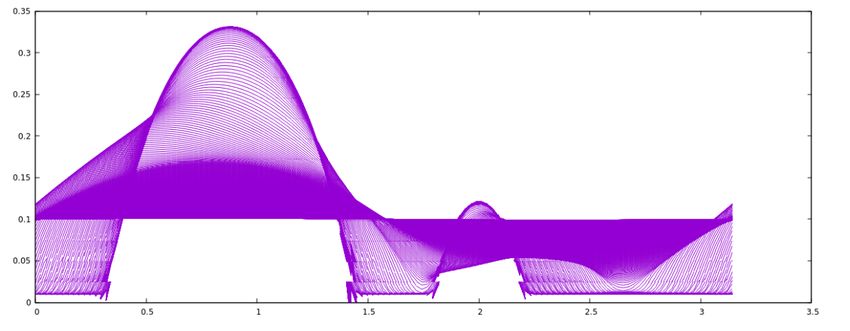
of the linear stability analysis [51]; see Fig. 6(a). 2) By making the bottom layer
slightly more viscous than the top layer, while the bilayer still remains unstable,
the nonlinear instability leads to the formation of a secondary droplet, suggest-
ing that even a small spatial variation of the viscosity can significantly alter the
instability characteristic length scales; see Fig. 6(b). 3) There appears to be a
correlation between the viscosity ratio and contact angle defining the threshold
for the formation of a secondary droplet; see Fig. 7.
8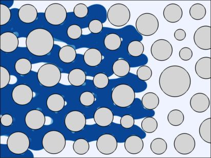
a0

                    wt
                            top layer
                                               µt

                                               µb
                    wb

                               bottom layer

                                                                                    h
                                               substrate

                                                     L

Figure 5: Schematic of the computational setup. Viscosity ratio is µb /µt , L is the wavelength
of a linearly unstable sinusoidal wave with an amplitude a0 , and h is the prewetted or precursor
film thickness.

                      (a)                                               (b)

Figure 6: Formation of a single drop (a) and two drops (b). L = π, wb = wt = 0.05, h = 0.01,
a0 = 1e-3, θ = 90◦ , and (a) µb /µt = 1 (b) µb /µt = 1.1 .

    Our future work will involve investigating film lengths, layer sequences, and
the influence of the surrounding viscosity. We will also further study the com-
positional structure of the bilayer systems. Our preliminary numerical results
reveal that the obtained final droplets have a composition of the two layers over
the whole volume of the droplets; while our results show qualitatively similar
distribution as illustrated in the experiments in [58], further analysis of the dif-
ferences in the composition as a function of the physical parameter set will help
tuning the morphology of such nanostructures for applications.

3. A multiscale model for the simulation of dynamic contact lines:
   the dewetting transition

   Here we review a recent work in [6] on the description of a method for dy-
namic contact lines. The work focuses on in-depth analysis on the physical

                                               9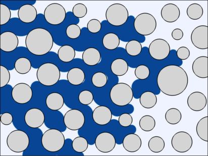
5.0

                                  4.5

                                  4.0

                                  3.5

                                  3.0
                Viscosity Ratio

                                  2.5                                 II
                                  2.0

                                  1.5              I
                                  1.0

                                  0.5

                                  0.0
                                    45   50   55   60   65    70     75    80    85    90   95   100   105   110

                                                             Contact Angle (Degrees)

Figure 7: The threshold for the formation of the secondary droplet (symbols), showing the
viscosity ratio µb /µt as a function of the contact angle θ. The geometrical parameters are the
same as in Fig. 6. Formation of a single drop (I) and two drops (II).

phenomenon of the dewetting transition. When modeling dynamic contact line,
here in the context of the VOF method, there are two major challenges: 1)
the numerical implementation of the contact angle, and 2) relieving the incom-
patibility between the moving contact line and the no-slip boundary condition
(see e.g. [60], for a recent mathematical view of the boundary conditions for dy-
namic wetting). In [6], the authors address both difficulties by first describing a
method to impose the contact angle as a boundary condition for when discretiz-
ing the surface tension in computational cells adjacent to the solid boundary,
and secondly, by devising an elaborate methodology to account for microscopic
features near the contact line, using an asymptotic theory for the solution of
the local contact line problem and to remove the singularity in the shear stress,
leading to numerical convergence. We note however that a fundamental question
still remains regarding the measurement of the microscopic contact angle and
its definition at a dynamic contact line, see e.g. [61] for a recent and renewed
discussion on the topic, and review papers [8, 54, 62].
     The discretization of Eq. 3 consists of two steps; first the reconstruction of
the interface followed by its advection. In the first part of the reconstruction
step, the interface normal n = (nx , ny ) in cel is determined from the values χ in
neighboring cells, using method described in [4, 23]. In the reconstruction step,
the position of a linear segment representing the interface in the cell is deter-
mined from the knowledge of n and χ [63]. The reconstructed linear segments
are updated in the advection step, where the interface is evolved by the fluid
velocity field, using Eq. 3.
     In order to compute capillary forces, we use the Height-Function method,
in which the local height of the interface is computed from summing over a
column of cells [4]. Using second-order finite differences of the local Height-

                                                                    10
Fluid 2,ρ2, µ2
Vs
h∞ g
h0 t=0
t
→ ∞
y Fluid 1,ρ1, µ1
x
Figure 8: Schematic illustrating the withdrawing plate setup.
Function then provides the curvature, as well as the interface normals, used
to compute the surface tension force (see [23, 24]). Near the contact line, the
interface is then linearly extended into the solid cell to prescribe the value
of χ function at ghost cells. Having the interface Heights (and Widths) now
defined at ghost cells, interface normal vector and curvature adjacent to the solid
boundary are computed as usual. Once the interface positions and the curvature
are computed, there is no special difficulty in computing the velocity field using
the standard methods. No special provision is made for the discontinuity of
velocities or the divergence of viscous stresses and pressures, which are computed
as elsewhere in the domain using finite volumes and finite differences. Intuitively,
this allows a kind of numerical slip. This numerical slip is studied in details in
[5].
3.1. Results
The problem setup is as follows: consider a solid plate being withdrawn
from a liquid reservoir with a constant velocity Vs > 0. The computational
domain is 0 ≤ x, y ≤ L, with fluid 1 occupying y < h0 and fluid 2 occupying
y > h0 at t = 0 (see Fig. 8). The viscosity and density of fluid i = 1, 2
are µi and ρi , respectively. The capillary number is defined as Ca = µ1 Vs /σ,
pσ the surface tension. We set L ≈ 9 lc ,
where µi is the viscosity of fluid i and
where lc is the capillary length lc = σ/[(ρ1 − ρ2 )g] with g the gravitational
acceleration. The Reynolds number is then defined based on the capillary length
as Re = ρ1 Vs lc /µ1 .
In [6], we focus on a specific, complex physical problem: the dewetting
transition. One example of such a flow is the withdrawing plate, see Fig. 8.
The interface may either sustain a stationary state meniscus, if below a critical
capillary number, Cacr , or continue to move up the substrate until depositing a
thin film to arbitrary heights. The latter is called a Landau–Levich–Derjaguin
(LLD) film [64, 65]. Figure 9 from [6] shows an example of the case where
Ca > Cacr . In [66–68], a hydrodynamic theory is developed for the prediction
of Cacr , while Cox [52] and Voinov [53] describe, on the other hand, how the
11(a)
(b)
(c)
12(d)
(e)
(f)
Figure 9: From [6]. Time evolution of the interface for Ca > Cacr at τ = Vs t/lc = 4 (a), 4.8
(b), 5.9 (c), 6.8 (d), 7.9 (e), 8.7 (f). The insets show the magnified flow field and the pressure
distribution. (a)-(c) Right panels show a magnified view of the contact line region and the
computational mesh; the fine structure of the flow field and the pressure distribution in the
contact line region are illustrated. Ca = 0.048, and θ = 60◦ . The pressure colors show the
maximum (dark red) and minimum (dark blue) of the pressure distribution.
13singularity drives a peculiar curved form of the fluid wedge at small Ca. In
[6], we use these theories to predict the numerically observed transition and to
devise a subgrid scale model to reproduce the underlying microscopic physics.
The latter reflects on the notion of grid-independent simulations in [5, 69]. In
the simulations, we measure Cacr and specify ∆, the typical grid size, and θ∆ ,
the specified contact angle at a particular grid size ∆. We compare the value
of Cacr from full simulations to the solutions of the central relation obtained in
[6, 70]
C(q)φ(θ∆ , q)Ca1/3
cr lc G(θ∆ )
exp − = 1, (10)
∆ Cacr
where the constant C(q) = O(1), q = µ2 /µ1 , G function is given in [52], and
φ = ∆/rm is the scaling factor or gauge function determined from the numerical
simulations by comparing to the analytical solutions, where we consider rm ∝ ∆,
namely the numerical slip. In [6, 70], the computed Cacr are in agreement with
the above solutions. Finally, it can be shown that
πeAi2 (smax ) ∆
G(θ∆ , q)
φ(θ∆ , q) = 1/3 −5/6 exp , (11)
3 2 Ca1/3
cr lc
Cacr
where Ai(x) is the Airy function of the first kind and Ai0 (smax ) = 0; see also an
earlier work in [71], where an expression similar to Eq. 11 is derive.
In Fig. 10, we plot the values of the right hand side of Eq. 11 along with
the computed values of φ. In the near-free-surface Setup C (q = 1/50), a very
clean estimate of the gauge function φ is obtained at small angles and we find
φ(θ∆ ) ' θ∆ . Thus our numerical model may be viewed as having an effective slip
of the order of a grid cell. However, we find that there is a mismatch between the
theory and the data in Eq. 11 in Fig. 10. If one leaves the connection between
the slip length λ and the grid size ∆ free, using λ = c∆ with c an arbitrary
constant, then the adjustable constant c allows a better fit of to the data; see,
for example, the dashed line ( ) in Fig. 10 for when choosing c = 3. This in
turn provides an estimate of the effective slip in our VOF method.
3.1.1. Recommendations for the numerical simulations of dynamic contact lines
As we discussed above, numerical slip plays a crucial role in numerical simu-
lations of the moving contact line problem. As shown, this numerical slip, which
is introduced at the discrete level, is effectively equivalent to a slip length on
the order of the grid size. Several authors have reported how this numerical slip
can strongly distort the results [5, 72, 73], unless the grid size in the vicinity of
the contact line is decreased to a microscopic scale, making the computations
prohibitively costly.
To develop a strategy for realistic simulations where experiments would be
used, the first step would be to perform a series of simulations at varying ∆ and
for the conditions of the experiments. Obviously, simulations and experiments
are not performed near the critical Ca but below it. Comparing the angles
observed in the region where the theory is still valid, would cross-validate the
1411
10
9
8
7
φ(θ∆)
6
5
4
3
2
1
0
0 0.2 0.4 0.6 0.8 1 1.2 1.4 1.6 1.8 2
θ∆
Figure 10: Using the data from [6, 70], φ is plotted using expression Eq. 11 for Setups A: q = 1
(×), B: Re = q = 1 (×), and C: q = 1/50 (×), compared to the computed values from the
best fit of φ for Setups A (•), B (•), and C (•), with θ∆ measured in radian. For a given angle
θ∆ , the various values of φ correspond to the various values of the grid size ∆ for each data
set. For all the simulations, the density ratio ρ1 /ρ2 = 5. The solid line ( ) is the prediction
from lubrication theory for φ = e θ∆ /3, when assuming λ ≈ ∆ and dashed line ( ), is for
when adjusting λ ≈ 3∆.
computations. This would in turn fix the parameters θ∆ and rm that could be
used in simulations. This approach is of course made difficult by the fact that
there is no evidence so far that a single pair θ∆ , rm could predict experiments
over a range of different flow configurations. Actually the authors of [74] state
that “In the literature we have not found a single pair of experiments in different
geometries using precisely the same materials.”. This highlights the difficulty of
a predictive simulation approach based on experiments. Moreover, it should be
noted that the authors of references [75] and [76] claim precisely the opposite,
that no microscopic angle, even a dynamical one depending on the capillary
number, can predict the whole range of experiments they have performed or
simulated. We therefore believe that the relationship between numerical slip
length and the grid size is strongly problem dependent. We provide such a
relation in Eq. 11 for the withdrawing plate problem in the hope that it moti-
vates further investigations for other scenarios, such as droplet impact on a solid
surface, where such relationships can also involve other relevant dimensionless
parameters such as Reynolds and Weber numbers. A suitable numerical slip
can then be identified by comparing the results with appropriate experimen-
15tal measurements. We note however again that such a relation might only be
applicable to that particular problem.
Finally, the slip boundary condition combined with a constant contact angle
might not sufficiently describe the dynamics of the moving contact line. In [26],
the authors propose to replace the slip boundary condition with a generalized
Navier boundary condition (GNBC) [77], coupled with a dynamic contact angle
to more favorably match the experimental observations in the context of the
curtain coating configuration [75] (see also [60, 78] for a recent discussion on the
boundary conditions for dynamic wetting).
4. Moving contact lines on arbitrary geometries
Numerically modeling non-ideal solid substrate is enormously complicated.
Wetting and spreading on rough surfaces, two-phase flow over topographically
patterned surfaces and through porous media are examples of such systems.
While there exist numerical studies on chemically disordered surfaces, see e.g. [79,
80], and with roughness effects in a two-phase flow model, see e.g. [81–83], pore-
scale numerical investigations are still scarce, see e.g. [84–86], and therefor in
what follows, we only focus on the direct numerical simulation of fluid–fluid
flows in a porous media model.
Pore-scale models have increasingly become a reliable tool for making pre-
dictions of two-phase flows through porous media; see e.g. [87, 88]. Direct
numerical simulation techniques based on solving the full Navier-Stokes equa-
tions provide an accurate solution for pore-scale analysis of multiphase flows in
porous media. However, a great challenge in pore-scale direct numerical sim-
ulations is the inclusion of wetting effects into the numerical model. There
exist direct numerical studies on pore-scale modeling of wettability effects, such
as the phase-field simulation in [89] and the lattice Boltzmann simulation in
[90]. While the majority of previous (Eulerian) interface capturing methods
include wetting on body-fitted meshes, less progress has been made to develop
numerical methods that handle arbitrary geometries (see e.g. [32]). To that end,
one attractive approach is the Immersed Boundary Method (IBM) [91, 92], be-
cause of its ability to model complex geometries, and its potential for modeling
systems of solid bodies with arbitrary relative motion [20]. Here we show an
accurate and robust numerical model developed in [93] and later extended in
[20] for combining wetting dynamics, in a VOF framework, and the IBM. Here
we briefly review the methodology developed in [93] as the basis of an IBM for
implementing wetting effects into the numerical model for arbitrary geometries.
The method developed in [93] is based on a ghost-cell Immersed Boundary
(IB) method for curved surfaces. In order to compute the interface curvature in
cells adjacent to an IB computational cell, the authors employ a method where
the IB stencil is modified to take into account the orientation of the interface
normal at the contact line to reflect the prescribed contact angle. The modified
stencil is illustrated in Fig. 11. At each point where the stencil intersects the
IB, the prescribed contact angle defines the value of the interface normal at the
contact line, ~ncl . Therefore, adjacent cells to the IB enter into the computation
16Figure 11: From [93]. The stencil used for the evaluation of curvature, κ, near the IB surface,
the normal to the interface at the contact line is determined from the prescribed contact angle.
of the curvature, κ, resulting in a wetting force that consequently enters the
surface tension discretization.
In [94], we present the results of an improved implementation of the above
method [20] to simulate two-phase flows in a porous media model. The results
are first of their kind in that they are obtained using a combined VOF/IBM
pore-scale direct numerical simulations to quantify the effects of the capillarity,
characterized by the capillary number, Ca, and wetting, characterized by the
contact angle, θ, on the displacement phenomena in a porous media model. In
Fig. 12, we show how wetting controls displacement patterns, and observe the
crossover from a stable propagating front to a fractal pattern, namely a fingering
instability. The results show that decreasing the contact angle leads to a change
of the flow behavior from strong fingering to stabilized front propagation, and
that the contact angle effect diminishes as Ca increases. As can be seen in Fig. 12
displacement patterns, for wetting invading fluids, the front propagates rather
smoothly, draining all of the displaced phase, while a non-wetting invading fluid
can lead to residual fluid.
5. Future direction: microlayer formation in nucleate boiling as an
example
Pool boiling is one of the most efficient mode of heat transfer, allowing a
wide range of systems to improve their thermal performance, from nuclear power
17Viscous fingering
-1
10
Capillary fingering
10-2
Ca
-3
10
Stable displacement
10-4
0 50 100 150
θ
Figure 12: From [94]. Displacement patterns at varying Ca and θ. Above a certain Ca
threshold only viscous fingering is visible for the parameters studied in this work.
plants to microelectronic devices [95]. Predicting boiling heat transfer however
is complicated by the need to resolve phenomena occurring over multiple scales
(see Fig.13), from the adsorbed liquid layer at the wall at the nanometer scale
up to the bubble size at the millimeter scale. Furthermore, a significant amount
of the total heat can be transferred within the micro-region (known as micro-
layer) near the contact line. Existing models of microlayer formation are often
physically incomplete, e.g. do not include the effect of surface tension or con-
tact angle. Moreover, the dynamics of the moving contact line has a profound
influence on the microlayer formation. Therefore, a general model on microlayer
formation must also resolve the motion of the contact line.
In [96], the authors present experimental and numerical observations of con-
tact line heat transfer in the framework of pool boiling and meniscus evapora-
tion. They focus on the influence of contact line dynamics on the local heat
transfer near the contact line suggesting that the heat transfer next to the con-
tact line is governed mainly by two mechanisms in superposition: microlayer
evaporation and transient conduction. In [97], the authors present a numerical
18Figure 13: From [96]. Multiple scales involved in nucleate boiling: from the millimeter scale
at the bubble cap to the nanometer scale at the adsorbed liquid layer.
framework in which a subgrid source of vapor is considered. In [98], the authors
present experimental results on the transition between contact line evaporation
and microlayer evaporation during the dewetting of a superheated wall. They
discuss the time resolved formation of the microlayer in detail and describe the
influence of the dewetting velocity, wall superheat, and heating power on the
microlayer formation. In [99], the authors describe the microlayer formation
as a dewetting transition in the presence of phase change and use the existing
theoretical, experimental and numerical data to a derive a specific criterion for
modeling the transition.
Here, we provide a review of the work in [97] of the procedure for direct
computations of nucleate boiling and the conditions under which the microlayer
is expected to form. In [97], we focus on numerical simulation of the hydro-
dynamics of bubble growth at a wall, and high resolution simulations of the
microlayer formation. We identify the minimum set of dimensionless param-
eters that controls microlayer formation, namely δ ∗ = f (r∗ , t∗ , Ca, θ) with δ ∗
the shape of the extended liquid microlayer, rc = µl /(ρl Ub ) and tc = rc /Ub the
characteristic length and time scales used, respectively, where Ub is the bubble
growth rate. We found that all three regions need to be modeled in order to
accurately represent the thickness of the microlayer. Central to our theory is
the results that the interface profile in the microlayer away from the contact
line can be qaccurately described (in the case of hemispherical bubble growth)
∗ ∗ as long as the motion of the contact line is negligible
as δ ≈ 0.5 r∗ − Rb,0
∗
compared to the bubble growth rate; Rb,0 is the dimensionless initial bubble
∗
radius and r is the dimensionless radial distance from the bubble root.
Experimental measurements of the earliest bubble growth rate (Fig. 14 (a))
and microlayer thickness (Fig. 14 (b)) are then used in [97] to validate the
numerical results, for the case of water at saturation at 0.101M P a. The nu-
merical results are compared with experimental results in Fig. 14 (b), showing
both qualitative and quantitative agreements. However, a departure from the
19(a) (b)
Figure 14: From: [97]. Measured bubble growth rates (black squares) over time (a); the
earliest bubble growth rate is measured at t = 20µs, showing that the initial bubble growth
rate during the first tens of µs may have been much higher than its first available measured
value of 4.2m/s. Two scenarios assumed for initial regimes: constant growth rate (blue dash-
dotted line), or constant acceleration (red dashed line). Thickness δ (in µm) measured in lab
experiment (black squares) of boiling water at saturation at 0.101M P a, 0.41ms after boiling
inception. The deduced microlayer thickness at t = 20µs (grey triangles) is obtained assuming
that the heat transfer within the microlayer is purely by conduction. The wall temperature at
boiling inception is 111.7◦ C, and the wall heat flux is 209kW/m2 . Predictions from the square
root model are plotted for the two initial profiles of Ub showed in (a). The first measured
value of Ub is Ub (t ∼ 20µs) ∼ 4.2m/s. For simulations: µl = 3.5 × 10⁻⁴ P a.s, ρl = 950kg/m3 .
model in the low thickness region is also observed. This discrepancy is expected
to be reduced if we no longer assume constant wall superheat, but include the
thermal coupling between the microlayer and the heated wall. Such coupling
would require to solve for the heat equation in the substrate. The initial evap-
oration of the microlayer would locally reduce the wall superheat and therefore
slow down the rate of evaporation of the microlayer. This slow-down effect of
the microlayer evaporation due to conjugate heat transfer with the solid surface
is currently not included in the results in Fig. 14, and must be a subject of fur-
ther investigation. In general, systematic experiments seem to be necessary to
validate the numerical model and to develop more applicable dynamic contact
line models.
5.1. Hot topics and future issues
Numerical challenges for dynamic contact lines amplify when including heat
and mass transfer mechanisms (i.e. evaporation, boiling, and condensation).
The numerical framework described in this review will face new challenges to
accurately and robustly implement the velocity discontinuity across the inter-
face due to the mass exchange. Including the conjugate heat transfer with the
solid substrate, which requires the coupling of the flow solver and the energy
20equations, as well as a domain decomposition strategy, introduces additional
challenges; see e.g.[100]. Here, we list some future issues:
• The continuum formulations for moving contact line models lay out a
strong foundation for studying such systems. We believe that more elab-
orate models that include microscopic phenomena are needed to calibrate
and verify numerical results towards building a more robust moving con-
tact line model.
• A static contact angle is not a compatible model to impose on a moving
contact line. We believe a dynamic contact angle model should address
a more physically correct model of the contact line, which is essential for
simulating real applications.
• Hybrid numerical models that include hydrodynamic theories of the dy-
namic contact line show promise. A more general theories to large contact
angles are needed to extend the applicability of such hybrid models. More-
over, a special attention should be given on the development of numerical
methods that include more level of details, still maintaining computational
efficiency.
• Extension of all the above items to textured surfaces poses a formidable
numerical challenge.
• This review provides an example of a powerful numerical tool, Gerris,
for studying relevant problems. While laying out a strong foundation,
more improved numerical methods should continue to be developed for
increasing the predictive power of direct simulations for real life engineer-
ing applications, especially for three-dimensional domains.
Acknowledgment
We acknowledge the support by the Petroleum Research Fund PRF-59641-
ND. We thank P. Lehrer for help with Basilisk computations, K. Mahady, for
fluid–fluid–solid interaction simulations, and S. Zaleski for fruitful discussions
and help with improving this review.
[1] P. de Gennes, Wetting: Statics and Dynamics, Rev. Mod. Phys. 57 (1985)
827.
[2] J. Jacqmin, Contact-line dynamics of a diffuse fluid interface, J. Fluid
Mech. 402 (2000) 57.
[3] P. D. Spelt, A level-set approach for simulations of flows with multiple
moving contact lines with hysteresis, J. Comput. Phys. 207 (2005) 389.
[4] S. Afkhami, M. Bussmann, Height functions for applying contact angles
to 2D VOF simulations, Int. J. Numer. Meth. Fluids 57 (2008) 453.
21[5] S. Afkhami, S. Zaleski, M. Bussmann, A mesh-dependent model for ap-
plying dynamic contact angles to VOF simulations, J. Comput. Phys. 228
(2009) 5370.
[6] S. Afkhami, J. Buongiorno, A. Guion, S. Popinet, Y. Saade, R. Scardovelli,
S. Zaleski, Transition in a numerical model of contact line dynamics and
forced dewetting, J. Comput. Phys. 374 (2018) 1061.
[7] Wörner, M., Numerical modeling of multiphase flows in microfluidics and
micro process engineering: a review of methods and applications, Mi-
crofluidics Nanofluidics 12 (2012) 841.
[8] Y. Sui, H. Ding, P. D. M. Spelt, Numerical simulations of flows with
moving contact lines, Annu. Rev. Fluid Mech. 46 (2014) 97.
[9] L. M. Pismen, Y. Pomeau, Disjoining potential and spreading of thin liq-
uid layers in the diffuse-interface model coupled to hydrodynamics, Phys.
Rev. E 62 (2000) 2480.
[10] Y. Pomeau, Recent progress in the moving contact line problem: a review,
Comptes Rendus Mécanique 330 (2002) 207.
[11] L. M. Pismen, B. Y. Rubinstein, Spreading of a wetting film under the
action of van der Waals forces, Phys. Fluids 12 (2000) 480.
[12] V. Starov, V. Kalinin, J.-D. Chen, Spreading of liquid drops over dry
surfaces, Adv. Colloid Interface Sci. 50 (1994) 187.
[13] M. Bussmann, J. Mostaghimi, S. Chandra, On a three-dimensional volume
tracking model of droplet impact, Phys. Fluids 11 (1999) 1406.
[14] H. Ding, P. D. M. Spelt, Wetting condition in diffuse interface simulations
of contact line motion, Phys. Rev. E 75 (2007) 046708.
[15] S. Afkhami, M. Bussmann, Height functions for applying contact angles
to 3D VOF simulations, Int. J. Numer. Meth. Fluids 61 (2009) 827.
[16] S. Shin, J. Chergui, D. Juric, Direct simulation of multiphase flows with
modeling of dynamic interface contact angle, Theor. Comput. Fluid Dyn.
32 (2018) 655.
[17] P. Yue, Thermodynamically consistent phase-field modelling of contact
angle hysteresis, J. Fluid Mech. 899 (2020) A15.
[18] H.-L. Li, H.-R. Liu, H. Ding, A fully 3D simulation of fluid-structure
interaction with dynamic wetting and contact angle hysteresis, J. Comput.
Phys. 420 (2020) 109709.
[19] T.-Y. Han, J. Zhang, H. Tan, M.-J. Ni, A consistent and parallelized height
function based scheme for applying contact angle to 3D volume-of-fluid
simulations, J. Comput. Phys. 433 (2021) 110190.
22[20] A. O’Brien, M. Bussmann, A moving immersed boundary method for
simulating particle interactions at fluid-fluid interfaces, J. Comput. Phys.
402 (2020) 109089.
[21] S. Popinet, The Gerris flow solver, http://gfs.sourceforge.net/, 1.3.2
(2012).
[22] S. Popinet, Gerris: a tree-based adaptive solver for the incompressible
Euler equations in complex geometries, J. Comput. Phys. 190 (2003) 572.
[23] S. Popinet, An accurate adaptive solver for surface-tension-driven inter-
facial flows, J. Comput. Phys. 228 (2009) 5838.
[24] S. Popinet, Numerical models of surface tension, Ann. Rev. Fluid Mech.
50 (2018) 49.
[25] S. Popinet, Basilisk, a free-software program for the solution of par-
tial differential equations on adaptive Cartesian meshes, http://basilisk.fr
(2018).
[26] T. Fullana, S. Zaleski, S. Popinet, Dynamic wetting failure in curtain
coating by the Volume-of-Fluid method, Eur. Phys. J. Special Topics 229
(2020) 1923.
[27] J. Sakakeeny, Y. Ling, Numerical study of natural oscillations of supported
drops with free and pinned contact lines, Phys. Fluids 33 (2021) 062109.
[28] T. D. Blake, The physics of moving wetting lines, J. Colloid Interface Sci.
299 (2006) 1.
[29] Y. Shikhmurzaev, Moving contact lines in liquid/liquid/solid systems, J.
Fluid Mech. 334 (1997) 211.
[30] C. Huh, L. E. Scriven, Hydrodynamic model of steady movement of a
solid/liquid/fluid contact line, J. Colloid Interface Sci. 35 (1971) 85.
[31] A. Dziedzic, M. Nakrani, B. Ezra, M. Syed, S. Popinet, S. Afkhami,
Breakup of finite-size liquid filaments: Transition from no-breakup to
breakup including substrate effects, Eur. Phys. J. E 42 (2019) 18.
[32] H. Liu, S. Krishnan, S. Marella, H. Udaykumar, Sharp interface Carte-
sian grid method II: A technique for simulating droplet interactions with
surfaces of arbitrary shape, J. Comput. Phys. 210 (2005) 32.
[33] J. Zhang, P. Yue, A level-set method for moving contact lines with contact
angle hysteresis, J. Comput. Phys. 418 (2020) 109636.
[34] J. W. Cahn, J. E. Hilliard, Free energy of a nonuniform system. 1. Inter-
facial free energy, J. Chem. Phys. 28 (1958) 258.
23[35] J. Jacqmin, Calculation of two-phase navier-stokes flows using phase field
modeling, J. Comp. Phys. 155 (1999) 96.
[36] J. Jacqmin, Onset of wetting failure in liquid-liquid systems, J. Fluid
Mech. 517 (2004) 209.
[37] P. Yue, C. Zhou, J. Feng, Sharp-interface limit of the Cahn-Hilliard model
for moving contact lines, J. Fluid Mech. 645 (2010) 279.
[38] D. Sibley, A. Nold, S. Kalliadasis, Unifying binary fluid diffuse-interface
models in the sharp interface limit, J. Fluid Mech. 736 (2013) 5.
[39] A. J. Briant, A. J. Wagner, J. M. Yeomans, Lattice boltzmann simulations
of contact line motion. i. liquid-gas systems, Phys. Rev. E. 69 (2004)
031602.
[40] T. Lee, L. Liu, Lattice boltzmann simulations of micron-scale drop impact
on dry surfaces, J. Comp. Phys. 229 (2010) 8045.
[41] T. Qian, X.-P. Wang, P. Sheng, Molecular scale contact line hydrodynam-
ics of immiscible flows, Phys. Rev. E 68 (2003) 016306.
[42] T. Qian, X.-P. Wang, P. Sheng, Molecular hydrodynamics of the moving
contact line in two-phase immiscible flows, Comm. Comput. Phys. 1 (2006)
1.
[43] T. Nguyen, M. Fuentes-Cabrera, J. Fowlkes, J. Diez, A. González,
L. Kondic, P. Rack, Competition between collapse and breakup in
nanometer-sized thin rings using molecular dynamics and continuum mod-
eling, Langmuir 28 (2012) 13960.
[44] M. Fuentes-Cabrera, B. Rhodes, J. Fowlkes, A. López-Benzanilla, H. Ter-
rones, M. Simpson, P. Rack, Molecular dynamics study of the dewet-
ting of copper on graphite and graphene: Implications for nanoscale self-
assembly, Phys. Rev. E 83 (2011) 041603.
[45] S. Afkhami, L. Kondic, Numerical simulation of ejected molten metal
nanoparticles liquified by laser irradiation: Interplay of geometry and
dewetting, Phys. Rev. Lett. 111 (2013) 034501.
[46] U. Lǎcis, P. Johansson, T. Fullana, B. Hess, G. Amberg, S. Bagheri, and
S. Zaleski, Steady moving contact line of water over a no-slip substrate,
Eur. Phys. J. Special Topics 229 (2020) 1897.
[47] W. Ren, W. E, Heterogeneous multiscale method for the modeling of
complex fluids and micro-fluidics, J. Comput. Phys. 204 (2005) 1.
[48] H. Huang, D. Liang, B. B. Wetton, Computation of a moving drop/bubble
on a slid surface using a front-tracking method, Commun. Math. Sci. 2
(2004) 535.
24[49] K. Mahady, S. Afkhami, L. Kondic, A volume of fluid method for simulat-
ing fluid/fluid interfaces in contact with solid boundaries, J. Comp. Phys.
294 (2015) 243.
[50] J. U. Brackbill, D. B. Kothe, C. Zemach, A continuum method for mod-
eling surface tension, J. Comput. Phys. 100 (1992) 335.
[51] K. Mahady, S. Afkhami, L. Kondic, A numerical approach for the direct
computation of flows including fluid-solid interaction: modeling contact
angle, film rupture, and dewetting, Phys. Fluids 28 (2016) 062002.
[52] R. G. Cox, The dynamics of the spreading of liquids on a solid surface.
Part 1. Viscous flow, J. Fluid Mech. 168 (1986) 169.
[53] O. Voinov, Hydrodynamics of wetting, Fluid Dynamics 11 (1976) 714.
[54] D. Bonn, J. Eggers, J. Indekeu, J. Meunier, E. Rolley, Wetting and spread-
ing, Rev. Mod. Phys. 81 (2009) 739.
[55] R. Seemann, S. Herminghaus, K. Jacobs, Gaining control of pattern for-
mation of dewetting liquid films, J. Phys. Condens. Matt. 21 (2001) 4925.
[56] C. Neto, K. Jacobs, R. Seemann, R. Blossey, J. Becker, G. Grün, Satellite
hole formation during dewetting: experiment and simulation, J. Phys.:
Condens. Matter 15 (2003) 3355.
[57] J. Becker, G. Grün, R. Seemann, H. Mantz, K. Jacobs, K. R. Mecke,
R. Blossey, Complex dewetting scenarios captured by thin-film models,
Nature Mat. 2 (2003) 59.
[58] Y. Oh, J. Lee, M. Lee, Fabrication of Ag-Au bimetallic nanoparticles by
laser-induced dewetting of bilayer films, Appl. Surf. Sci. 434 (2018) 1293.
[59] D. A. Garfinkel, G. Pakeltis, N. Tang, I. N. Ivanov, J. D. Fowlkes, D. A. G.,
P. D. Rack, Optical and magnetic properties of ag–ni bimetallic nanopar-
ticles assembled via pulsed laser-induced dewetting, ACS Omega 5 (2020)
19285.
[60] M. Fricke, D. Bothe, Boundary conditions for dynamic wetting - A math-
ematical analysis, Eur. Phys. J. Special Topics 229 (2020) 1849.
[61] S. Afkhami, T. Gambaryan-Roisman, L. M. Pismen, Challenges in
nanoscale physics of wetting phenomena, Eur. Phys. J. Special Topics
229 (2020) 1735.
[62] J. H. Snoeijer, B. Andreotti, Moving contact lines: Scales, regimes, and
dynamical transitions, Annu. Rev. Fluid Mech. 45 (2013) 269.
[63] G. Tryggvason, R. Scardovelli, S. Zaleski, Direct Numerical Simulations
of Gas-Liquid Multiphase Flows, Cambridge University Press, 2011.
25[64] L. D. Landau, B. V. Levich, Dragging of a liquid by a moving plate, Acta
Physicochim. URSS 17 (1942) 42.
[65] B. V. Derjaguin, On the thickness of a layer of liquid remaining on the
walls of vessels after their emptying, and the theory of the application of
photoemulsion after coating on the cine film, Acta Physicochim. URSS 20
(1943) 349.
[66] J. Eggers, Hydrodynamic theory of forced dewetting, Phys. Rev. Lett. 93
(2004) 094502.
[67] J. Eggers, Contact line motion for partially wetting fluids, Phys. Rev. E
72 (2005) 061605.
[68] T. S. Chan, J. H. Snoeijer, J. Eggers, Theory of the forced wetting tran-
sition, Phys. Fluids 24 (2012) 072104.
[69] D. Legendre, M. Maglio, Comparison between numerical models for the
simulation of moving contact lines, Comput. Fluids 113 (2015) 2.
[70] S. Afkhami, J. Buongiorno, A. Guion, S. Popinet, Y. Saade, R. Scardovelli,
S. Zaleski, Corrigendum to “Transition in a numerical model of contact
line dynamics and forced dewetting” [J. Comput. Phys. 374(2018)1061–
1093], J. Comput. Phys. 382 (2019) 61.
[71] J. Qin, P. Gao, Asymptotic theory of fluid entrainment in dip coating, J.
Fluid Mech. 844 (2018) 1026.
[72] J. A. Moriarty, L. W. Schwartz, Effective slip in numerical calculations of
moving-contact-line problems, J. Eng. Math. 26 (1992) 81.
[73] O. Weinstein, L. M. Pismen, Scale dependence of contact line computa-
tions, Math. Model. Nat. Phenom. 3 (2008) 98.
[74] P. Yue, J. J. Feng, Wall energy relaxation in the Cahn-Hilliard model for
moving contact lines, Phys. Fluids 23 (2011) 012106.
[75] T. Blake, M. Bracke, Y. Shikhmurzaev, Experimental evidence of nonlocal
hydrodynamic influence on the dynamic contact angle, Phys. Fluids 11
(1999) 1995.
[76] M. Wilson, J. Summers, Y. Shikhmurzaev, A. Clarke, T. Blake, Nonlocal
hydrodynamic influence on the dynamic contact angle: Slip models versus
experiment, Phys. Rev. E 73 (2006) 041606.
[77] T. Qian, X.-P. Wang, P. Sheng, Generalized Navier boundary condition
for the moving contact line, Commun. Math. Sci. 1 (2003) 333.
[78] M. Fricke, M. Köhne, D. Bothe, A kinematic evolution equation for the
dynamic contact angle and some consequences, Phys. D: Nonlinear Phe-
nom. 394 (2019) 26.
26You can also read