Effects of turbulence structure and urbanization on the heavy haze pollution process
←
→
Page content transcription
If your browser does not render page correctly, please read the page content below
Atmos. Chem. Phys., 19, 1041–1057, 2019
https://doi.org/10.5194/acp-19-1041-2019
© Author(s) 2019. This work is distributed under
the Creative Commons Attribution 4.0 License.

Effects of turbulence structure and urbanization on the heavy
haze pollution process
Yan Ren1 , Hongsheng Zhang1 , Wei Wei2 , Bingui Wu3 , Xuhui Cai4 , and Yu Song4
1 Laboratory for Climate and Ocean-Atmosphere Studies, Department of Atmospheric and Oceanic Sciences, School of
Physics, Peking University, Beijing 100081, P.R. China
2 State Key Laboratory of Severe Weather, Chinese Academy of Meteorological Sciences, Beijing 100081, P.R. China
3 Tianjin Municipal Meteorological Bureau, Tianjin 300074, P.R. China
4 State Key Joint Laboratory of Environmental Simulation and Pollution Control, Department of Environmental Science,

Peking University, Beijing 100081, P.R. China

Correspondence: Hongsheng Zhang (hsdq@pku.edu.cn)

Received: 28 August 2018 – Discussion started: 28 September 2018
Revised: 18 December 2018 – Accepted: 8 January 2019 – Published: 28 January 2019

Abstract. In this paper, an automated algorithm is devel-         urban areas is much greater than on urban areas. The turbu-
oped, which is used to identify the spectral gap during           lent effects caused by urbanization seem to help reduce the
the heavy haze pollution process, reconstruct acquired data,      consequences of pollution under the same weather and pollu-
and obtain pure turbulence data. Comparisons of the recon-        tion source condition, because the turbulence intermittency is
structed turbulent flux and eddy covariance (EC) flux show        weaker, and the reduction in turbulence exchange is smaller
that there are overestimations regarding the exchange be-         over the urban underlying surface.
tween the surface and the atmosphere during heavy haze pol-
lution episodes. After reconstruction via the automated algo-
rithm, pure turbulence data can be obtained. We introduce
a definition to characterize the local intermittent strength of   1   Introduction
turbulence (LIST). The trend in the LIST during pollution
episodes shows that when pollution is more intense, the LIST      PM2.5 (fine particular matter, with a diameter smaller than
is smaller, and intermittency is stronger; when pollution is      2.5 µm) has become the foremost pollution issue in China
weaker, the LIST is larger, and intermittency is weaker. At       (Zhang et al., 2012; Hu et al., 2014), particularly in Bei-
the same time, the LIST at the city site is greater than at the   jing and its vicinity, in terms of severity and duration (Watts,
suburban site, which means that intermittency over the com-       2005; Tang et al., 2009, 2012, 2015; Zhang et al., 2014; Yang
plex city area is weaker than over the flat terrain area. Ur-     et al., 2015). Because of its negative impacts on human health
banization seems to reduce intermittency during heavy haze        (Dominici et al., 2014; Thompson et al., 2014) and compli-
pollution episodes, which means that urbanization reduces         cated effects on weather and climate (Liepert et al., 2004;
the degree of weakening in turbulent exchange during pol-         Wang et al., 2010, 2015a, b; Q. Zhang et al., 2015), heavy
lution episodes. This result is confirmed by comparing the        aerosol pollution has prompted the close attention of not only
average diurnal variations in turbulent fluxes at urban and       scientists but also the government and ordinary people.
suburban sites during polluted and clean periods. The sen-           During pollution periods, previous studies have indicated
sible heat flux, latent heat flux, momentum flux, and turbu-      that meteorological conditions always include constant stag-
lent kinetic energy (TKE) in urban and suburban areas are         nant winds, relatively increased water-vapour density, and
all affected when pollution occurs. Material and energy ex-       strong stable stratification, which inhibits the diffusion of
changes between the surface and the atmosphere are inhib-         vertical pollution and results in the explosive growth of
ited. Moreover, the impact of the pollution process on sub-       PM2.5 in Beijing (L. Zhang et al., 2015; R. Zhang et al., 2015;
                                                                  Wei et al., 2018; Zhong et al., 2018). The diurnal variations

Published by Copernicus Publications on behalf of the European Geosciences Union.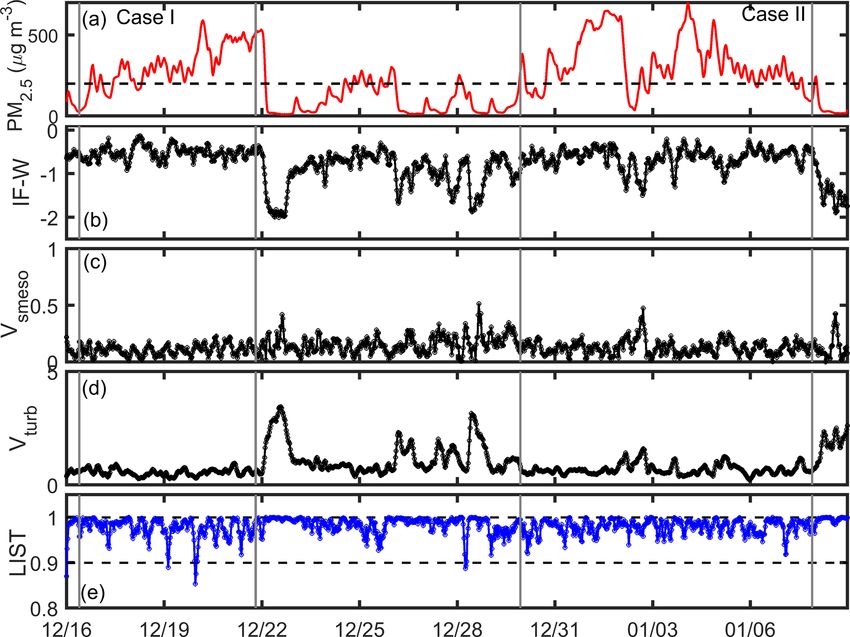
1042                                                 Y. Ren et al.: Effects of turbulence structure on the heavy haze process

in particulate concentrations are mostly dominated by the di-      process (Li et al., 2016). To provide a basis for improving the
urnal variability of the boundary layer and source emissions       parameterization scheme of the atmospheric pollution diffu-
(Liu et al., 2014); turbulent motion determines the meteoro-       sion model, it is very important to accurately calculate pure
logical elements in the atmospheric boundary layer, such as        turbulent transport during the heavy pollution process.
turbulence diffusion, PBL height, and atmospheric circula-            Therefore, the purpose of this study is to separate clas-
tion patterns, are all key to hazy weather (Wang et al., 2015a,    sic turbulent motions from submesoscale motions. At the
b; Tang et al., 2016; Zhu et al., 2018; Zhang et al., 2016) and    same time, intermittency can be defined by the turbulent and
dominate whether the haze occurs or not, since emissions           nonturbulent portions of a signal once the criteria for iden-
can remain stable within a defined period in a certain area.       tifying the boundary between them have been established
Therefore, the spatial and temporal characteristics of turbu-      (Salmond, 2005). Only in this way can we identify the classic
lent activity have significant effects on the local air quality    turbulence exchange during pollution periods, regardless of
from hourly to diurnal scales under a stable boundary layer        whether turbulence occurs over a flat underlying surface or
(Salmond and McKendry, 2005).                                      a complex underlying surface. In a previous study, Muschin-
   Turbulence in the stable boundary layer is weak and typi-       ski (2004) found a plateau in the intermittency spectra. Vick-
cally characterized by intermittent turbulence or even no tur-     ers and Mahrt (2003) showed the existence of a cospec-
bulence at a variety of heights, temporal scales, and spatial      tral gap, which separated turbulent and mesoscale contri-
locations (Mahrt, 1998, 2014; Coulter and Doran, 2002; Van         butions to calculate the fluxes in heat, moisture, and mo-
de Wiel et al., 2003; Salmond, 2005). The term intermit-           mentum using the multiresolution decomposition technique.
tency has different meanings that vary among studies (Coul-        Salmond (2005) used the wavelet analysis to objectively iso-
ter and Doran, 2002; Muschinski et al., 2004; Acevedo et           late intermittent turbulent bursts within vertical velocity time
al., 2006; Mahrt, 2007a). Mahrt (1989, 1999) defines inter-        series. Wei et al. (2017) found that the spectral gap sepa-
mittency as the case where eddies at all scales are missing or     rates fine-scale turbulence from large-scale motions using the
suppressed at scales that are large compared to those for large    arbitrary-order Hilbert spectral analysis during intermittency
eddies. A number of studies have indicated that intermittency      in the Cooperative Atmosphere–Surface Exchange Study-
is driven by nonstationarity due to motion on timescales that      1999 (CASE-99). Because of the nonstationarity and nonlin-
are slightly greater than those for turbulence (Mahrt, 2007a,      earity of intermittent turbulence, analytical techniques have
2010b) when the large-scale flow is weak. These motions            significant impacts on the results. A new technique, named
are sometimes referred to as submesoscale motions (Nappo,          the arbitrary-order Hilbert spectral analysis (Huang et al.,
2002; Sun et al., 2004; Anfossi et al., 2005; Conangla et al.,     2011), showed its advantage and validity in the application
2008; Mahrt et al., 2008). Some studies have simply defined        of turbulent flow and intermittency (Wei et al., 2016, 2017,
intermittency as “another name for nonstationary” (Treviño,        2018).
2000).                                                                In this paper, we use the arbitrary-order Hilbert spectral
   As mentioned earlier, the occurrence of heavy haze is al-       method to analyse turbulence data observed during several
ways accompanied by low wind speeds and strong stable              severe haze pollution episodes that occurred in Beijing and
stratification. Under these conditions, exchanges between the      its nearby suburbs from 16 December 2016 to 8 January 2017
surface and the atmosphere cannot be calculated with the           to identify the spectral gap and separate classic turbulence
eddy-correlation technique when intermittent turbulence ex-        from the original signal. After obtaining the pure turbulence
ists because of the nonstationarity imposed by submesoscale        signal and the strength of the submesoscale motions, the clas-
motions (Vickers and Mahrt, 2006; Acevedo et al., 2006,            sic turbulent flux and intermittency strength can be calcu-
2007; Aubinet, 2008; Mahrt, 2010a), which makes it very            lated. Then, we can obtain the macrostatistical characteristics
difficult to accurately determine the transport, storage, and      of turbulence over a flat terrain in suburban Beijing and dis-
diffusion of pollutants, particularly in regions with complex      cover the difference between clean and polluted days. This
terrain (Bowen et al., 2000), such as Beijing. Densely con-        analysis is helpful for improving the current understanding
structed buildings on the underlying surface aggravate the         of the transport and diffusion of PM2.5 and the intermittency
complexity of turbulent exchange during pollution periods,         strength of turbulence when heavy haze pollution occurs. The
and the impact of urbanization on pollution is unknown. The        effect of urbanization on the heavy pollution process is si-
Monin–Obukhov similarity theory establishes the relation-          multaneously studied by comparing the results of the urban
ship between turbulent flux and the vertical gradient in the       and suburban sites.
surface layer and has been widely used in weather and cli-
mate models (Wood et al., 2010; Wilson, 2008). However,
turbulent flux calculated by the traditional time-averaging
method is contaminated by submesoscale motions during the
heavy pollution process, which makes the application of sim-
ilar theories difficult and may be the reason that the simulated
pollutant concentration is lower during the heavy pollution

Atmos. Chem. Phys., 19, 1041–1057, 2019                                             www.atmos-chem-phys.net/19/1041/2019/
Y. Ren et al.: Effects of turbulence structure on the heavy haze process 1043
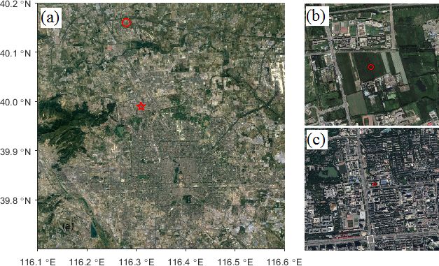
Figure 1. Google Earth map of the observation sites in Beijing: (a) the observation site located in the urban underlying surface region
(marked by the red pentagram) and the observation site located in the suburban underlying surface region with a flat terrain (marked by the
red circle). The corresponding terrains (within a range of approximately 1 km) around the observation sites are shown in (b) and (c).
2 Description of the sites and data sit facilities that surround the station. The site is located in
a typical urban landscape. The buildings around the site are
2.1 Experimental site neat and uniform, and the average building height is 20 m.
So observations at the urban site are located within the sur-
face layer. Details on the site introduction and data back-
The data used in this paper are from two measurement ground have been shown in Ren et al. (2018). The concen-
sites (Fig. 1 shows the location of the two sites). Data over trations of PM2.5 were collected using a Thermo Fisher Sci-
a flat terrain were collected at a continuous measurement entific instrument (series FH-62-C14), and 30 min averag-
site (40.16◦ N, 116.28◦ E) in a Beijing suburb. The obser- ing time series were performed to remove outliers. The sys-
vational site was set up in the middle of a vast and hori- tem was equipped with an integrated CO2 /H2 O open-path
zontal farmland, near the Changping county. A 10 m tower gas analyzer (LI-7500, LI-COR Biosciences, Inc., USA) and
was erected for the eddy covariance (EC) and meteorologi- three-dimensional sonic anemometer-thermometer (IRGA-
cal measurements. The EC system was mounted at a height SON, Campbell Scientific, Inc., USA). The IRGASON was
of 8.3 m above ground, which was located within the surface levelled and pointed north. The turbulence data such as the
layer. The system was equipped with an integrated CO2 – horizontal wind vector, virtual temperature, and water vapour
H2 O open-path gas analyzer and three-dimensional sonic content were collected using a data logger (CR3000, Camp-
anemometer-thermometer (IRGASON, Campbell Scientific, bell Scientific, Inc., USA) at a frequency of 10 Hz and were
Inc., USA). The IRGASON was levelled and pointed north. averaged over an interval of 30 min for the analysis of mete-
The turbulence data, such as the horizontal wind vector, orological elements. For convenience of description, this site
virtual temperature, and water vapour content, were col- is described as the urban site.
lected using a data logger (CR3000, Campbell Scientific, The suburban site is 20 km away from the urban site. At
Inc., USA) at a frequency of 10 Hz and were averaged over this distance, the large-scale weather background is consis-
an interval of 30 min for the analysis of meteorological ele- tent. Because of the flat terrain of the suburban site, it was
ments. For convenience of description, this site is described used as a reference. The sources of PM2.5 of the two sites
as the suburban site. are generally consistent. The observations of PM2.5 at urban
The second data set was collected over urban terrain at a sites are used to represent the evolution of the entire pollution
continuous measurement site at Peking University (39.99◦ N, process, as this study focuses on pollution processes rather
116.31◦ E) in Beijing, which is the capital of China. The in- than specific values. Since the observations at both sites are
struments are situated on top of a building at the School of located in the surface layer, i.e., the constant flux layer, the
Physics (Peking University) and extend 25 m above ground. values of turbulence flux are comparable.
There are teaching and residential buildings and public tran-
www.atmos-chem-phys.net/19/1041/2019/ Atmos. Chem. Phys., 19, 1041–1057, 2019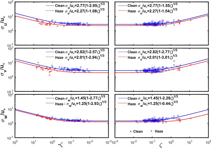
1044                                                      Y. Ren et al.: Effects of turbulence structure on the heavy haze process

2.2    Data processing

In this study, we select a 24-day pollution period from 16 De-           σu = u0 u0 ,
cember 2016 to 8 January 2017; the number of heavy pollu-
                                                                         σv = v 0 v 0 ,
tion days with PM2.5 concentrations exceeding 200 µg m−3
reached 15 (17–21, 24–25, 28, and 30–31 December 2016                    σw = w 0 w 0 ,
and 1–7 January 2017). The remaining days were identified                σθ = θ 0 θ 0 ,
as clear days. The PM2.5 mass concentration, horizontal wind
speed, virtual temperature, and water vapour mixing ratio are            σq = q 0 q 0 ,                                                    (2)
shown in Fig. 2 for the days of concern. The trends in me-
teorological elements over time are consistent at both sites.            the turbulence flux is calculated as
The horizontal wind speed is larger during clear days and
                                                                         τ = ρu2∗ = ρu0 w0 ,
smaller during pollution days; the virtual temperature seems
to be greater during pollution days, but this result is not obvi-        H = ρCp w 0 θ 0 ,
ous. The water-vapour content is significantly higher during             E = ρw0 q 0                                                       (3)
pollution days than during clear days. The characteristics of
these meteorological elements during the pollution process               and the friction speed is calculated as
are similar to those in previous studies (Wang et al., 2014;
Sun et al., 2014; Tai et al., 2010).                                                         2                    2  14
   The raw turbulence data were preprocessed over an av-                 u∗ =        −u0 w 0        +       −v 0 w0             .          (4)
eraging interval of 30 min by the Eddy Pro software (Ad-
vanced 4.2.1, LI-COR Biosciences, Inc., USA). Preprocess-                3.2    Automated algorithm to identify the spectral gap
ing included procedures involving error flags, despiking (fol-
lowing Vickers and Mahrt, 1997), double rotations (follow-               In the traditional turbulence theory, Van der Hoven (1957)
ing Wilczak et al., 2001), and detrending, which are im-                 presented an analysis on the large spectrum of horizontal
plemented using the block-averaging method. In this paper,               wind speeds, which showed a notable spectral gap of ap-
the EC method is used to calculate the flux for comparison,              proximately 1 cycle h−1 between the macroscale (synoptic)
where the average time is 30 min. At the same time, strict               and microscale (turbulent) parts of the spectrum. Many other
quality control is performed on the data and data groups to              studies have generally proven the existence of the spectral
remove data meeting any of the following conditions: (1) the             gap (Panofsky, 1969; Fiedler and Panofsky, 1970; Smedman-
EC method runs with more than ±120◦ between the wind                     Högström and Högström, 1975). As observations progressed,
direction and direction of the sonic anemometer, (2) the in-             many studies on the stable boundary layer have indicated
cluded angle between the wind direction and horizontal plane             that the turbulent part of the signal decreases, the timescale
is greater than 3◦ , (3) the wind speed is less than 0.5 m s−1 ,         for turbulence decreases, and the timescale for the spectral
(4) the friction speed is less than 0.05 m s−1 , (5) the sensi-          gap also decreases, as mentioned above. These studies used
ble heat flux is less than 5 W m−2 , and (6) data groups are             the multiresolution decomposition method to choose a vari-
obviously incorrect.                                                     able averaging time to remove the effects of mesoscale mo-
                                                                         tions. The method we used here to separate pure turbulence
                                                                         and submesoscale motion is based on half-hourly data (i.e.,
3     Methodology
                                                                         the fixed averaging time). The multiresolution basis utilized
3.1    Turbulent kinetic energy and turbulent fluxes                     is a wavelet set, as it is the only wavelet set that satisfies
                                                                         Reynolds averaging (Howell and Mahrt, 1997; Mallat, 1998;
The physical quantities used in this paper are turbulent ki-             Vickers and Mahrt, 2003, 2006). In this study, we adopt the
netic energy (TKE), several variances (σu , σv , σw , σθ , and           Hilbert–Huang transform (Huang et al., 1998, 1999), which
σq ), friction speed (u∗ ), and fluxes (−u0 w 0 , w0 θ 0 and w0 q 0 ).   is fully data-driven and local in both the physical and fre-
Among these, the TKE is calculated as                                    quency domains (Huang et al., 1998; Flandrin et al., 2004).
                                                                         The advantages of researching turbulence data that are non-
      1  02
                                                                         stationary and nonlinear have been proven previously (Huang
e=       u + v 0 2 + w0 2 ,                                       (1)
      2                                                                  et al., 2008, 2013; Schmitt et al., 2009; Wei et al., 2013, 2016,
                                                                         2017).
the variance is calculated as
                                                                            The spectral gap was examined by studying the second-
                                                                         order Hilbert spectra (u0 , v 0 , w0 , θ 0 , and q 0 ) for each 30 min
                                                                         period. The calculation method for the second-order Hilbert
                                                                         spectra comes from the arbitrary-order Hilbert spectral anal-
                                                                         ysis (Huang et al., 2008), which is an extended version

Atmos. Chem. Phys., 19, 1041–1057, 2019                                                         www.atmos-chem-phys.net/19/1041/2019/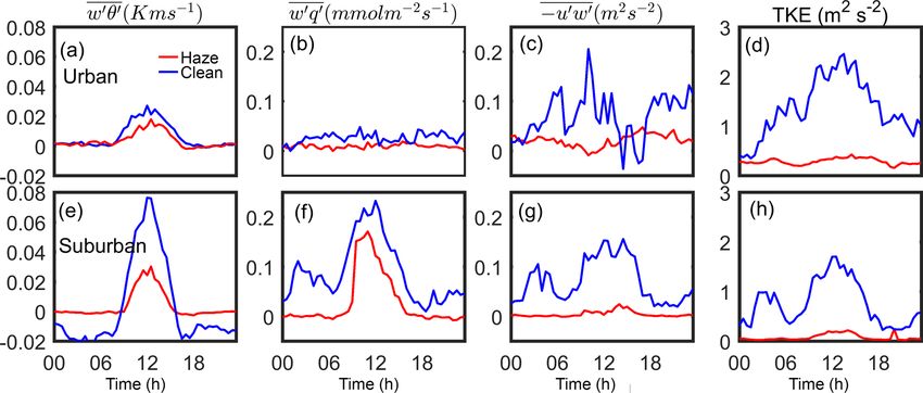
Y. Ren et al.: Effects of turbulence structure on the heavy haze process                                                                1045

Figure 2. The PM2.5 mass concentration (a), horizontal wind speed (b), virtual temperature (c), and water-vapour mixing ratio (d) from
16 December 2016 to 8 January 2017. The black solid line represents data from the suburbs of Beijing (flat terrain), and the black dotted line
represents data from the Peking University site (urban landscape).

of the Hilbert–Huang transform. A joint probability den-                 data. The part of the frequency larger than ω indicates the
sity function (PDF), p(ω, A), can be extracted from ωi                   turbulence signal, and the part of the frequency smaller than
and Ai for all intrinsic mode functions. Then, the arbitrary-            ω indicates nonstationary motion, which has a scale larger
order Hilbert marginal spectrum is defined as an amplitude-              than that for turbulence. Then, we can search for the mode of
frequency space by the marginal integration of the joint PDF             the intrinsic mode function (IMF) (N = 9 in this case), which
p(ω, A):                                                                 has the mean frequency closest to ω. Therefore, modes 1–N
         Z                                                               are chosen to reconstruct the pure turbulence signal, and the
Lq (ω) = p(ω, A)Aq dA,                                    (5)            remaining modes are chosen to reconstruct the signal of the
                                                                         submesoscale motion.
where ω represents the instantaneous frequency, A represents                As shown in Figs. 3a–c, it is obvious that the reconstruc-
the instantaneous amplitude, q ≥ 0 represents the arbitrary              tion successfully eliminated the energy contained by large-
moment, and p(ω, A) represents the PDF. Specifically, h(ω)               scale motion while retaining turbulent energy. The new spec-
corresponds to theRsecond-order Hilbert marginal spectrum                trum, which is shown by the black dotted lines in Fig. 3, is
(h (ω) = L2 (ω) = p(ω, A)A2 dA).                                         consistent with the structure of the turbulent energy spectrum
   An automated algorithm was developed to objectively find              in the classic theory. We reconstructed the data for all time
the frequency location of the spectral gap. This method is               periods when the spectral gap existed in our data set. The re-
based on the characteristics in Fig. 4b in Wei et al. (2017).            sults of the total reconstructed data spectrum showed that the
The spectral gap between turbulence and the submesoscale                 whole process removed the effects of large-scale motion and
motions is identified as the frequency interval in which the             retained classic turbulence, while simultaneously obtaining
second-order Hilbert spectral values are approximately con-              large-scale motions.
stant, or the slope is approximately equal to 0. Figure 3
shows the second-order Hilbert spectra from the newly re-                3.3    The local intermittent strength of turbulence
constructed data and raw data. As shown in Fig. 3a, the
lower-frequency limit of the spectral gap is ω = 0.008 Hz,               We use the ratio of turbulent intensity compared to all signals
and the upper-frequency limit is not used to reconstruct the             to indicate the intermittent strength. To obtain the strength

www.atmos-chem-phys.net/19/1041/2019/                                                       Atmos. Chem. Phys., 19, 1041–1057, 2019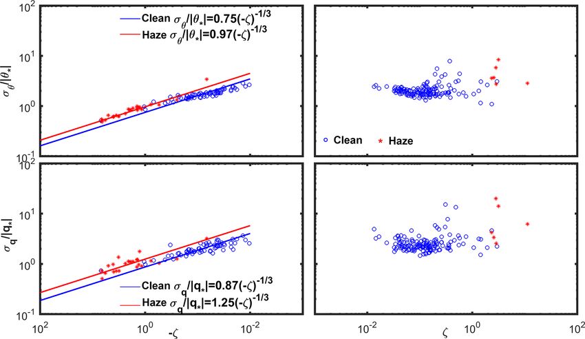
1046                                                         Y. Ren et al.: Effects of turbulence structure on the heavy haze process

                                                                            during each 30 min period. Then, we can define the local in-
                                                                            termittent strength from an energy point of view as follows:

                                                                                           Vturb
                                                                            LIST = q                     .                               (8)
                                                                                          2
                                                                                        Vsmeso     2
                                                                                               + Vturb

                                                                            The value of the LIST is equal to the ratio of turbulent inten-
                                                                            sity in the acquired signal. When the LIST is large and close
                                                                            to 1, there are more turbulent components in the acquired sig-
                                                                            nal, the influence of the submesoscale motion is weaker, and
                                                                            the intermittency is weaker. When the LIST is small and far
                                                                            from 1, there are fewer turbulent components in the collected
                                                                            signal, the influence of submesoscale motion is stronger, and
                                                                            the intermittency is stronger.

                                                                            4     Results and discussion

                                                                            4.1    Comparison of the macro-statistical parameters for
                                                                                   reconstructed turbulence and the results of the
                                                                                   fixed averaging time

                                                                            We use the automated algorithm to identify the spectral gaps
                                                                            in 1152 groups of 10 Hz high-frequency data from 16 De-
                                                                            cember 2016 to 8 January 2017 at the urban and suburban
                                                                            sites. There are 440 groups of data in the along-wind di-
                                                                            rection, 519 groups of data in the cross-wind direction, 390
                                                                            groups of data in the vertical direction, 467 groups of data in
                                                                            the scalar θ , and 501 groups of data in the scalar q, which
                                                                            is where the spectral gap occurs at the suburban site. The
                                                                            data sets encompassing the spectral gap account for 38 %,
                                                                            45 %, 34 %, 41 %, and 43 % of the total data at the subur-
Figure 3. Second-order Hilbert spectra of three wind speed com-
                                                                            ban site, respectively. The proportions are 41 % (481), 37 %
ponents U (a), V (b), and W (c) at 08:00 on 31 December 2016 at
the suburban site. The black solid line indicates the spectra from the      (425), 35 % (402), 41 % (476), and 45 % (520) for the u, v,
raw data, and the black dotted line indicates the spectra from the          w, t, and q components at the urban site. The occurrence of
reconstructed data for pure turbulence. The solid gray lines indicate       a spectral gap is common throughout the pollution process,
the position of the spectral gap.                                           which means that the effects of nonstationary motion on the
                                                                            collected signals are common throughout the process. Under
                                                                            these conditions, the usual half-hour length is not suitable
of submesoscale motion, we introduce the definition of the                  for stationary conditions. The eddy-correlation flux calcu-
velocity scale for submesoscale motion from Mahrt (2007b,                   lated using a conventional averaging time of 30 min to define
2009, 2010b, 2011). The velocity scale for submesoscale mo-                 the perturbations is severely contaminated by poorly sampled
tion represents the kinetic energy of submesoscale motions                  mesoscale motions.
and is defined as follows:                                                     During the half-hour period, we refer to the variance in
                                                                            the pure turbulent fluctuations as the new results and that
          q
Vsmeso = u0 2smeso + v 0 2smeso + w 0 2smeso ,           (6)                calculated via the classic EC system is referred to as the
where u0 smeso , v 0 smeso , and w0 smeso , represent the deviations        original variance results. A comparison of the TKE and vari-
reconstructed from the IMF corresponding to the subme-                      ance parameters (σu , σv , σw , σθ , and σq ) between the new
soscale motions during each 30 min period. Similarly, the tur-              results and original results is shown in Fig. 4, and a com-
bulent velocity scale is defined as follows:                                parison among the vertical heat flux (w0 θ 0 ), vertical water-
        q                                                                   vapour flux (w0 q 0 ), and momentum flux (−u0 w0 ) is presented
Vturb = u0 2turb + v 0 2turb + w 0 2turb ,                       (7)        in Fig. 5; the fitted lines are given in both figures. When there
                                                                            is no spectral gap, the 30 min time length is suitable for sta-
where u0 turb , v 0 turb , and w 0 turb , represent the deviations recon-   tionary conditions; therefore, the classic EC method is cred-
structed from the IMF corresponding to the turbulent motions                ible. Figures 4 and 5 only present the results when there is a

Atmos. Chem. Phys., 19, 1041–1057, 2019                                                       www.atmos-chem-phys.net/19/1041/2019/
Y. Ren et al.: Effects of turbulence structure on the heavy haze process 1047
spectral gap (i.e., when there is nonstationarity at the subur- timate the flux between land surfaces and the atmosphere
ban site). (Baldocchi, 2003). Under weak-stability conditions, eddy-
All of the fitted results show that there are certain degrees correlation fluxes calculated using a conventional averag-
of overestimated variance in Fig. 4. The slope of the fitted ing time of 5 min or longer to define the perturbations are
line is 0.81 for the TKE, as Fig. 4f shows, which means that severely contaminated by poorly sampled mesoscale motions
the TKE originally calculated by the conventional method (Vickers and Mahrt, 2006). The average block time that has
is overestimated by approximately 19 %. The comparison of been used is 30 min, which has been used in practice since
σu and σv shows the same pattern as that for the TKE. The Kaimal and Finnigan (1994), who proposed that a 30 min
traditional method for the half-hourly eddy correlation over- averaging time was a reasonable compromise for daytime
estimates by approximately 27 % (slope of 0.73) and 21 % analyses. From the above analysis, we can see that turbulent
(slope of 0.79) for σu and σv , respectively. The overestima- fluxes are overestimated due to the effects of submesoscale
tion of σw is not as obvious as those for σu and σv . The slope motions when there is a spectral gap. During the heavy
of the fitted line in Fig. 4c is 0.99, which indicates that the haze pollution process, turbulence is weak, which causes
appearance of the spectral gap has fewer effects on the vari- this overestimation to become even more apparent. Zhong
ance in vertical velocity. The overestimation is even more et al. (2017, 2018) proposed that heavy pollution events in
pronounced when the TKE and σu , σv , and σw are small, Beijing are characterized by the transport stage (TS), with a
which indicates that the overestimation can be more signif- formation of aerosol pollution primarily caused by pollutants
icant when the turbulence is weak. Similarly, we examine transported from regions south of Beijing, and the cumulative
the variance in potential temperature and moisture content stage (CS), where the cumulative explosive growth in PM2.5
in Fig. 4d and e. The variations in potential temperature and mass concentration is dominated by stable stratification char-
moisture content are also overestimated: the difference is that acteristics in the atmosphere, such as slight or calm souther-
the overestimation percentages are larger. The slopes of the lies, anomalous inversions near the ground, and moisture ac-
fitted lines in Fig. 4d and e are 0.60 and 0.54, which means cumulation. According to the classification criteria for the CS
that the traditional method for the half-hourly eddy correla- and TS, we briefly compared the characteristics of turbulent
tion overestimates approximately 40 % and 46 % of σθ and fluctuation, variance, and flux at different times during the
σq when the spectral gap occurs. Such a substantial overes- pollution process from 15 to 23 December 2016, as shown in
timation cannot be ignored. In general, the variations in σu , Fig. 6. Due to the consistent patterns of different variables,
σv , σw , σθ , and σq calculated by the traditional EC method only the results for horizontal velocity are shown in this pa-
for 30 min are all overestimated, especially when the turbu- per. We can clearly see from Fig. 6 that the turbulent fluctu-
lence is weak, due to the impact of submesoscale motion. ation, variance, heat flux, and momentum flux are obviously
In addition, the overestimation in the horizontal direction is smaller during polluted periods (CS and TS) than those dur-
more significant than in the vertical direction. However, the ing clean periods. Therefore, the exchange of fluxes between
overestimation of these quantities cannot be ignored. the ground and atmosphere can be easily overestimated with
After separating pure turbulence and submesoscale motion the traditional eddy-correlation method during the pollution
from the signal, the pure turbulent flux can be calculated dur- process, which can result in false forecasts of contaminant
ing heavy haze pollution periods. The comparison of the pure concentrations and pollution levels. Some works have found
turbulent flux with the flux calculated by the eddy-correlation that current pollution forecasts tend to underestimate pollu-
method at a fixed averaging time is presented in Fig. 5. The tant concentrations (Li et al., 2016). The overestimation of
momentum flux, −u0 w 0 , is overestimated by approximately turbulent flux during heavy pollution episodes may be one of
13 %, and the slope of the fitted line in Fig. 5c is approx- the reasons for this result.
imately equal to 0.87. The effect of nonstationary motion
on heat transfer and water-vapour transfer is similar to that 4.2 The relationship between the local intermittent
on momentum, as seen in Fig. 5. Overestimation can reach strength and pollution
12 % (slope of 0.88) and 15 % (slope of 0.85) for w0 θ 0 and
w0 q 0 in Fig. 5a and b. The reconstructed turbulence data re- After reconstruction via the automated algorithm, pure turbu-
sults at the urban site show that the traditional half-hourly lent data can be obtained. The LIST from 16 December 2016
eddy-correlation results have a certain degree of overestima- to 8 January 2017 is discussed in this section. We calculated
tion regarding the turbulent fluxes and variances during the the LIST of the urban and suburban sites separately and dis-
pollution period. However, the degree of overestimation in cussed the relationship between the LIST and degree of pol-
urban areas is less than in suburban areas. A comparison of lution.
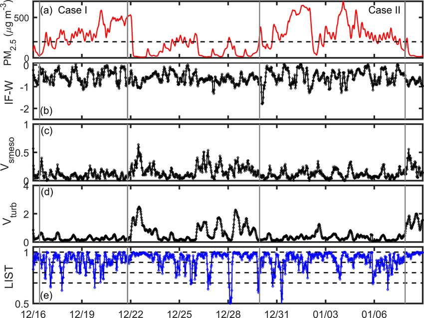
the macrostatistical parameters for turbulence from the new Figure 7 shows the time series for (a) PM2.5 concentra-
half-hourly results with those from the original results at the tions, (b) the intermittency factor (IF) of vertical velocity,
city site is not shown here. (c) the velocity scale for submesoscale motions (Vsmeso ),
In the majority of recent research, the EC technique has (d) the velocity scale for turbulence (Vturb ), and (e) the LIST
become the most frequently used method with which to es- for turbulence from 16 December 2016 to 8 January 2017
www.atmos-chem-phys.net/19/1041/2019/ Atmos. Chem. Phys., 19, 1041–1057, 20191048 Y. Ren et al.: Effects of turbulence structure on the heavy haze process Figure 4. Comparison of σu (a), σv (b), σw (c), σθ (d), σq (e), and TKE (f) from the new half-hour results with those from the original results from 16 December 2016 to 8 January 2017 at the suburban site. The black dotted line represents the 1 : 1 line in the figures. The black solid line represents the fitted results. Figure 5. A comparison of the vertical heat flux (w0 θ 0 ) (a), vertical water-vapour flux (w 0 q 0 ) (b), and momentum flux (−u0 w0 ) (c) from the new half-hourly results with those from the original results from 16 December 2016 to 8 January 2017 at the suburban site. The black dotted line represents the 1 : 1 line in the figure. The black solid line represents the fitted results. at the suburban site. Figure 8 shows the results of the same intensity of the submesoscale motion is weaker than dur- variables at the city site. Wei et al. (2018) has shown that ing the clean period, and the energy of the turbulent flow there is a relationship between the IF, which characterizes is also weaker. Correspondingly, the local intermittent inten- the intensity of intermittent mixing, and the concentration sity is strong, as the LIST is farther from 1. Specifically, of PM2.5 . In this section, we also present the IF of the ver- for the period of explosive growth in pollutant concentra- tical wind speed in Figs. 7b and 8b to discuss internal re- tion (CS) during the two pollution processes of Case I and lations and differences with the local intermittent strength. Case II in Fig. 7, the intermittent intensity (LIST) is signif- Low PM2.5 concentrations correspond to large values of IF, icantly stronger (weaker) than during the clean period and Vsmeso , and Vturb , and weak intermittent intensity (i.e., the other weak pollution events, with a concentration of approx- LIST is closer to 1) in Figs. 7 and 8. The decrease in PM2.5 imately 200 µg m−3 . The two processes, Case I and Case II, concentration corresponds to the increases in IF, Vsmeso , and are similar in that both experience a rapid decline in the con- Vturb and the decrease in local intermittent intensity. For sev- centration of PM2.5 (from a heavy pollution level greater than eral heavy pollution events with PM2.5 concentrations higher 500 µg m−3 to one less than 30 µg m−3 ) on a timescale of than 200 µg m−3 , the absolute value of the IF is smaller, the several hours. The difference is that there is a clean period Atmos. Chem. Phys., 19, 1041–1057, 2019 www.atmos-chem-phys.net/19/1041/2019/
Y. Ren et al.: Effects of turbulence structure on the heavy haze process                                                             1049

Figure 6. Time series of (a) PM2.5 concentration, (b) horizontal wind speed, (c) variation in horizontal wind speed, (d) vertical heat flux
(w0 θ 0 ), and (e) momentum flux (−u0 w0 ) from 15 to 23 December 2016 at the suburban site.

approximately 1 day after the rapid decline in the Case I pro-             From the analysis of the clean and polluted periods, we
cess, but in the Case II process, the PM2.5 concentration de-           can see that the submesoscale motion persists throughout the
creases sharply in just a few hours and then rapidly increases          30 min acquired signal. During heavily polluted periods, the
to the 600 µg m−3 level. By comparing the rapid reduction               intensity of turbulence is weak, and the effects of subme-
in the PM2.5 concentrations during the Case I and Case II               soscale motion on weak turbulence begin to appear. Dur-
processes, we find that there is no significant difference in           ing clean periods, the intensity of turbulence is strong, and
submesoscale motion strength, whereas turbulent intensity               the effect of submesoscale motion is relatively small. Mean-
during the Case I process is significantly greater than dur-            while, the submesoscale motion is a source of turbulent en-
ing the Case II process, which leads to a weaker (stronger)             ergy when the turbulence is very weak under heavy pollu-
LIST during the Case I (Case II). During the Case II pro-               tion and stable weather conditions. It can be said that turbu-
cess, although the LIST (intermittent intensity) increases (de-         lence derives energy from nonstationary, large-scale motion
creases) when the PM2.5 concentration begins to decrease,               and has a very large effect on the concentration of pollutants
the larger (weaker) LIST (intermittent intensity) is not main-          over timescales of hours (e.g., Case I and Case II). We also
tained but decreases (increases) rapidly, which indicates that          note the relationship between LIST and IF. Wei et al. (2018)
the pollutant concentration does not fully diffuse and rapidly          mentioned that the larger the absolute value of the IF is, the
increases again to 600 µg m−3 within a few hours. The differ-           stronger the intermittent mixing. From the perspective of in-
ence between these two processes also indicates that the dif-           termittent mixing strength, the IF tends to be consistent with
fusion of pollutants directly depends on the diffusion of tur-          the LIST defined in this paper. When the pollutant concen-
bulent flow during heavy pollution processes. Submesoscale              trations decreased sharply, intermittent mixing increased, the
motion may be an important source of turbulent energy un-               IF absolute value increased, the LIST (intermittent intensity)
der stable weather conditions, but it is not directly involved          increased (decreased), and turbulent exchange was enhanced.
in the dissipation of pollutants.                                          The tendency of the LIST under pollution conditions in
                                                                        Fig. 8 is consistent with that in Fig. 7, which indicates that the

www.atmos-chem-phys.net/19/1041/2019/                                                     Atmos. Chem. Phys., 19, 1041–1057, 2019
1050 Y. Ren et al.: Effects of turbulence structure on the heavy haze process
Figure 7. Time series of the (a) PM2.5 concentrations, (b) intermittency factor (IF) of vertical velocity, (c) velocity scale of submesoscale
motions (Vsmeso ), (d) velocity scale of turbulence (Vturb ), and (e) LIST from 16 December 2016 to 8 January 2017 at the suburban site.
above analysis conclusions apply not only to suburban sites for turbulence, and the normalized standard deviations in po-
but also to urban sites. However, there is a significant differ- tential temperature and water vapour under near-neutral con-
ence between the urban and suburban sites: the LIST (inter- ditions are closer to those of Panofsky et al. (1984) and Wyn-
mittent intensity) at suburban sites is weaker (stronger) than gaard (1971). The figures regarding the macrostatistical char-
at urban sites. The value of Vsmeso at the city site is slightly acteristics of turbulence before reconstruction are not shown
smaller than at the suburban site, and the value of Vturb at the here.
city site is larger than at the suburban site. Correspondingly, Figure 9 shows that under both polluted and clear weather
the value of the LIST at the city site is significantly greater conditions, the relations of the normalized standard devia-
than at the suburban site, which means that the dynamic ef- tions in horizontal and vertical wind speeds with the stabil-
fect of the underlying surface of the urban area is stronger ity parameter ζ follows the one-third power law well un-
than that of the flat underlying surface of the suburban area. der stable and unstable stratification conditions. The normal-
Next, in Sect. 4.3 and 4.4, we verify the results from the sta- ized standard deviation was more dispersed in the horizon-
tistical characteristics of turbulence and the daily changes in tal direction than in the vertical direction, which is consis-
turbulent flux during polluted and clear periods, respectively. tent with the results presented in Zhang et al. (2004) and
Ma et al. (2002) and shows that the physical characteris-
4.3 Macrostatistical characteristics of turbulence tics of the land surface (e.g., topography and roughness)
affect the statistical properties of the vertical wind speed
Figures 9 and 10 show the relationship of the normalized less than those of the horizontal wind speed. The normal-
standard deviations in wind speed in the horizontal and verti- ized standard deviations in the horizontal and vertical wind
cal directions (σu /u∗ , σv /u∗ , and σw /u∗ ) with potential tem- speeds are nearly constant under near-neutral conditions (i.e.,
perature (σθ / |θ∗ |) and moisture content (σq / |q∗ |) as func- −0.01 < ζ < 0.01), and the constants are slightly larger than
tions of the stability parameter ζ at the suburban site, respec- those from Panofsky et al. (1984), which is similar to the
tively. It should be noted that the reconstructions of the data results from other suburban works (i.e., Zhang et al., 1991;
have two benefits. One is that the discrete situation of the Roth et al., 1993; Su et al., 1994). Figure 9 shows that the val-
fitted line has been significantly improved after reconstruc- ues during clean periods (circle) are slightly larger than those
tion. The other is that the statistical characteristics of turbu- during haze periods (asterisk) under unstable conditions. Ren
lence are more consistent with the classic statistical pattern et al. (2018) (Fig. 4) show the significant difference in the
Atmos. Chem. Phys., 19, 1041–1057, 2019 www.atmos-chem-phys.net/19/1041/2019/Y. Ren et al.: Effects of turbulence structure on the heavy haze process 1051 Figure 8. Time series of the (a) PM2.5 concentrations, (b) intermittency factor (IF) of vertical velocity, (c) velocity scale of submesoscale motions (Vsmeso ), (d) velocity scale of turbulence (Vturb ), and (e) LIST from 16 December 2016 to 8 January 2017 at the city site. normalized standard deviations in the horizontal and verti- lution process has a more significant influence on the tur- cal wind speeds between clear and haze periods. The recon- bulent statistical characteristics of potential temperature and structed data from the city site also show the same conclusion moisture in the suburbs and a less significant impact on those (the figures are not shown in this paper), which means that in the urban area. the dynamic effect of turbulence during pollution episodes is reduced significantly at both the city and suburban sites. At 4.4 The impact of urbanization on turbulent transport the same time, the normalized standard deviations in wind during heavy pollution episodes speed in three directions over the suburban area are smaller than those over urban areas under near-neutral conditions, Figure 11 shows the diurnal variations in the mean w0 θ 0 , which shows that the dynamic effect of turbulence at the ur- w 0 q 0 , −u0 w 0 and TKE under both polluted weather and clear ban site is stronger than at the suburban site. weather conditions. The sensible heat flux (vertical heat flux) Figure 10 shows the relationships of the normalized exhibits unimodal diurnal variations during both clean and standard deviations in potential temperature and moisture polluted periods over either the suburban site or city site, with the stability parameter ζ . Given unstable stratification, as shown in Fig. 11a and e. During the clean period, the σθ / |θ∗ | and σq / |q∗ | fit the function ζ −1/3 . The fitting coef- peak in the daily sensible heat flux at the suburban site ap- ficients are larger than the typical value of 0.95 presented in pears around 12:00 noon (local time), reaching a maximum Wyngaard (1971), which used data from a grassland area in of 0.07 K m s−1 ; the peak in the daily sensible heat flux at the Kansas (United States). Similarly to the conclusion for the urban site also appears around 12:00 noon, with a peak value normalized standard deviations in the three-directional wind close to 0.04 K m s−1 , which is less than that in the subur- speeds, Ren et al. (2018) (Fig. 5) shows the slight differences ban area. One possible reason is that the buildings in the ur- in the normalized standard deviations in potential tempera- ban area are denser and have higher reflectivity, resulting in ture between clear and haze periods, while Fig. 10 in this less net radiation and, consequently, a lower peak in the sen- paper shows a significant difference between clear and haze sible heat flux. Another difference in the sensible heat flux periods. Since the time periods studied are the same, the dif- between the city and suburban sites during the clean period ference in the performance of these turbulence statistics dur- is that the sensible heat flux over the suburbs is negative at ing polluted and clean periods over city and suburban sites night, with a downward heat transfer, but not in urban areas. indicates the impact of urbanization. In other words, the pol- This pattern may be due to the emission of anthropogenic www.atmos-chem-phys.net/19/1041/2019/ Atmos. Chem. Phys., 19, 1041–1057, 2019
1052                                                       Y. Ren et al.: Effects of turbulence structure on the heavy haze process

Figure 9. Normalized standard deviations in wind speed in the horizontal and vertical directions (σu /u∗ , σv /u∗ , and σw /u∗ ) as functions
of the stability parameter ζ . The red (blue) line in the figure represents the results under polluted (clear) weather conditions. Observations
marked with ∗(◦ ) were made under polluted (clear) weather conditions.

Figure 10. Normalized standard deviations in the potential temperature (σθ / |θ∗ |) and moisture content (σq / |q∗ |) as functions of the stability
parameter ζ . The red (blue) line in the figure represents the results under polluted (clear) weather conditions. Observations marked with ∗(◦ )
were made under polluted (clear) weather conditions.

heat sources at nighttime in cities and the difficulty of dis-              flux is not completely below zero. Previous research on city
sipating heat over tall and dense buildings; therefore, there               and suburban sites in Helsinki also found the same features
is not a vast temperature difference between the surface of                 (Nordbo et al., 2013). During the pollution period, the peak
the city and the upper air and, accordingly, the sensible heat              in sensible heat flux at the urban site dropped to approxi-

Atmos. Chem. Phys., 19, 1041–1057, 2019                                                        www.atmos-chem-phys.net/19/1041/2019/
Y. Ren et al.: Effects of turbulence structure on the heavy haze process                                                                      1053

Figure 11. Diurnal variations in the mean vertical heat flux (w 0 θ 0 ) (a), vertical water-vapour flux (w 0 q 0 ) (b), momentum flux (−u0 w0 ) (c),
and TKE (d) under polluted weather (red solid line) and clear weather (blue solid line) conditions over the urban site. Diurnal variations in
these variables over the suburban site are shown in (e), (f), (g), and (h).

mately 0.02 K m s−1 . In addition, other trends were exactly                period, the momentum fluxes at the urban and suburban sites
the same as those during the clean period. At the same time,                are significantly lower than those during the clean period and
the peak in sensible heat flux at the suburban site dropped                 remain low throughout the day. However, at this time, the
to 0.02 K m s−1 , and the daily change in sensible heat flux                momentum flux over the city is greater than over the sub-
was somewhat different than during the clean period (i.e.,                  urbs, as Fig. 11c and g show. The change in TKE is similar
the characteristic of downward sensible heat flux at night                  to that in momentum flux. During the clean period, the TKE
disappeared completely). In general, pollution caused a re-                 values over the urban and suburban sites all showed obvious
duction in the upward transport of sensible heat flux, and it               unimodal diurnal variations. The TKE values over the urban
had a weaker impact on the city and a stronger impact on the                area were greater than those over the suburban area, which is
suburbs. In addition, pollution can also hinder the downward                due to the strong turbulence in wake vortices caused by un-
transmission of nighttime sensible heat flux in the suburbs.                derlying surfaces, such as high buildings in urban areas. Dur-
   The daily changes in latent heat flux over the urban and                 ing the pollution process, the urban and suburban TKEs both
suburban areas are completely different. During the clean pe-               decreased significantly and remained low throughout the day.
riod, the latent heat flux at the city site (Fig. 11b, dotted line)         However, the TKE over the city site was still greater than
does not have obvious daily variations and fluctuates at ap-                over the suburban site.
proximately 0, which is related to low winter temperatures,                    Based on the above analysis, we know that the sensible
the presence of water in the form of solid ice, and very dry                heat flux and latent heat flux of the urban site are less than
air. However, the daily changes in latent heat in the suburbs               those of the suburban site, and the momentum transport and
during the clean period show a unimodal change, reaching                    TKE of the urban areas are greater than those of the subur-
a peak at approximately 12:00 noon. It seems that the pollu-                ban sites due to different underlying surfaces. The sensible
tion process has no significant effect on the transport of latent           heat flux, latent heat flux, momentum flux, and TKE in the
heat over the urban area. As the solid line in Fig. 11b shows,              urban and suburban areas are all affected when pollution oc-
the latent heat flux over the urban area during the pollution               curs. Pollution inhibits the material and energy exchanges be-
period remains low, fluctuating at approximately 0. However,                tween the surface and atmosphere. Moreover, the impact of
the pollution process has a greater impact on the transfer of               the pollution process on the suburbs is much greater than on
latent heat in the suburbs. As shown by the dotted line in                  the urban area. If the turbulent structure over the flat surface
Fig. 11f, the transfer of latent heat is reduced throughout the             of the suburban area is considered the normal state for tur-
day.                                                                        bulent structures in this area during the studied period, then
   The magnitude of the momentum flux is related to the                     the urban turbulent structure is influenced by urbanization.
roughness of the underlying surface, wind speed, and stabil-                From this perspective, urbanization has reduced the impact
ity of the boundary layer. During the clean period, the mo-                 of pollution on water and heat exchanges between the sur-
mentum flux over the city site experiences a wide range of                  face and atmosphere. In conjunction with Sect. 4.2, the value
changes, and the peak value is larger due to the high rough-                of the LIST in urban areas is greater than in suburban areas,
ness of the city’s underlying surface; the suburban momen-                  which means that the intermittent intensity of urban turbu-
tum flux also has obvious daily changes, but the peak value                 lence is less than that of suburban turbulence. Therefore, the
is slightly lower than over the city site. During the pollution             turbulence signal over the urban site is stronger than over the

www.atmos-chem-phys.net/19/1041/2019/                                                           Atmos. Chem. Phys., 19, 1041–1057, 2019
1054                                                   Y. Ren et al.: Effects of turbulence structure on the heavy haze process

suburban site, and pollution in urban areas is weaker than in        from those at the city site. These conclusions are consistent
adjacent suburbs.                                                    with the diurnal variations in mean flux under both polluted
                                                                     weather and clear weather conditions at the city site and sub-
                                                                     urban site. The sensible heat flux, latent heat flux, momen-
5   Conclusions and discussions                                      tum flux, and TKE over the urban and suburban areas are all
                                                                     affected when pollution occurs. Due to the close distance be-
In this paper, we developed an automated algorithm to iden-          tween the two stations, the large-scale weather background is
tify the spectral gap to separate pure turbulence and subme-         consistent, and the suburban site is locally flat, so the turbu-
soscale motions from a 30 min signal based on the arbitrary-         lent structure over the flat surface of the suburban area is con-
order Hilbert spectral method. We used this automated algo-          sidered the normal state in this area under such weather and
rithm to analyse turbulence data observed from several se-           pollution source conditions; then the urban turbulent struc-
vere haze pollution episodes in Beijing and its nearby sub-          ture is influenced by urbanization. More importantly, the re-
urbs from 16 December 2016 to 8 January 2017. The data               duction in turbulence exchange during the pollution period
sets with a spectral gap accounted for approximately 30 % of         in suburban sites is greater compared to urban sites. In other
the total data, indicating that the eddy-correlation flux calcu-     words, the impact of the pollution process on the suburbs
lated using a conventional averaging time of 30 min to de-           is much greater than on the urban area. The change in the
fine perturbations is severely contaminated by poorly sam-           underlying surface of the urban site (the dynamic effect of
pled mesoscale motions. Due to space limitations, only the           complex terrain and the heat island effect caused by human
detailed suburban site results are listed in the text. The re-       activities) leads to a greater resistance to the weakening ef-
sults of the urban site are consistent with the conclusions of       fects of turbulent exchange caused by pollution.
the suburban site. A comparison between the reconstructed
variances of u0 , v 0 , w0 , θ 0 , and q 0 and those calculated by
the conventional method revealed overestimations of approx-          Data availability. Data used in this study are available from the
imately 27 %, 21 %, 1 %, 40 %, and 46 %, when there was a            corresponding author upon request (hsdq@pku.edu.cn).
spectral gap. The vertical wind speed was overestimated less
than the horizontal wind speed. The scalar, potential temper-
atures were overestimated more than the wind speed vector.           Author contributions. YR and HZ determined the goal of this
The calculations of the fluxes were also overestimated. The          study. YR carried it out, analyzed the data and prepared the paper
                                                                     with contributions from all co-authors. WW helped to figure out the
momentum flux, heat flux, and water-vapour flux were over-
                                                                     methodological problem based on HHT. BW, XC and YS designed
estimated by approximately 13 %, 12 %, and 15 %. We can              the field experiment, carried them out and got the data. All authors
see from these comparisons that the overestimation of flux           contributed to the discussion and interpretation of the results and to
during haze events cannot be ignored.                                article modifications.
   After reconstruction via the automated algorithm, pure tur-
bulent data can be obtained. Then, we explore the relation-
ship between the LIST and pollution. The results indicate            Competing interests. The authors declare that they have no conflict
that, when pollution is heavy, the LIST is smaller, and the in-      of interest.
termittency is stronger; when pollution is lighter, the LIST is
larger, and the intermittency is weaker. During the heavy pol-
lution process, air quality is determined by turbulent motion        Acknowledgements. This work was jointly funded by grants from
on the hourly scale. At the same time, the LIST at the city site     National Key R&D Program of China (2016YFC0203300) and
is greater than at the suburban site, which means that the in-       the National Natural Science Foundation of China (91544216,
termittency over the complex city surface is weaker than over        41705003, 41675018, 41475007).
the flat terrain of the suburbs. Urbanization seems to reduce
                                                                     Edited by: Jianping Huang
the intermittency during heavy haze pollution episodes. The
                                                                     Reviewed by: two anonymous referees
results were validated via the statistics on the impact of ur-
banization on turbulence and turbulent transport during pol-
luted and clean periods.
   The results for the statistical characteristics of turbulence
show a significant difference in the normalized standard de-         References
viations in the horizontal and vertical wind speeds between
                                                                     Acevedo, O. C., Moraes, O. L. L., Degrazia, G. A., and Medeiros,
clear and haze periods at the suburban site, which is the same         L. E.: Intermittency and the exchange of scalars in the
as that at the city site; significant differences in the normal-       nocturnal surface layer, Bound.-Lay. Meteorol., 119, 41–55,
ized standard deviations in potential temperature and water-           https://doi.org/10.1007/s10546-005-9019-3, 2006.
vapour content between clear and haze periods are also ob-           Acevedo, O. C., Moraes, O. L. L., Fitzjarrald, D. R., Sakai,
served at the suburban site, which are substantially different         R. K., and Mahrt, L.: Turbulent carbon exchange in

Atmos. Chem. Phys., 19, 1041–1057, 2019                                                 www.atmos-chem-phys.net/19/1041/2019/
Y. Ren et al.: Effects of turbulence structure on the heavy haze process 1055 very stable conditions, Bound.-Lay. Meteorol., 125, 49–61, the Hilbert-Huang transform, Phys. Rev. E, 87, 041003, https://doi.org/10.1007/s10546-007-9193-6, 2007. https://doi.org/10.1103/PhysRevE.87.041003, 2013. Anfossi, D., Oettl, D., Degrazia, G., and Goulart, A.: An Huang, Y. X., Schmitt, F. G., Hermand, J. P., Gagne, Y., Lu, Z. M., analysis of sonic anemometer observations in low wind and Liu, Y. L.: Arbitrary-order Hilbert spectral analysis for time speed conditions, Bound.-Lay. Meteorol., 114, 179–203, series possessing scaling statistics: Comparison study with de- https://doi.org/10.1007/s10546-004-1984-4, 2005. trended fluctuation analysis and wavelet leaders, Phys. Rev. E, Aubinet, M.: Eddy Covariance CO2 Flux Measurements in Noc- 84, 16208, https://doi.org/10.1103/PhysRevE.84.016208, 2011. turnal Conditions: An Analysis of the Problem, Ecol. Appl., 18, Kaimal, J. C. and Finnigan, J. J.: Atmospheric boundary layer flows: 1368-1378, https://doi.org/10.1890/06-1336.1, 2008. Their structure and measurement, Oxford University Press, New Baldocchi, D.: Assessing the eddy covariance technique for York, 255–261, 1994. evaluating carbon dioxide exchange rates of ecosystems: Li, T., Wang, H., Zhao, T., Xue, M., Wang, Y., Che, H., and Jiang, past, present and future, Glob. Change Biol., 9, 479–492, C.: The Impacts of Different PBL Schemes on the Simulation of https://doi.org/10.1002/(SICI)1096-8652(199710)56:23.0.CO;2- PM2.5 during Severe Haze Episodes in the Jing–Jin–Ji Region Y, 2003. and Its Surroundings in China, Adv. Meteorol., 2016, 62958778, Bowen, B. M., Baars, J. A., and Stone, G. L.: Nocturnal Wind Di- https://doi.org/10.1155/2016/6295878, 2016. rection Shear and Its Potential Impact on Pollutant Transport, Liepert, B. G., Feichter, J., Lohmann, U., and Roeckner, E.: Can J. Appl. Meteorol., 39, 165–233, https://doi.org/10.1175/1520- aerosols spin down the water cycle in a warmer and moister 0450(2000)0392.0.CO;2, 2000. world?, Geophys. Res. Lett., 31, 177–182, 2004. Conangla, L., Cuxart, J., and Soler, M. R.: Characterisation of the Liu, Z., Hu, B., Wang, L., Wu, F., Gao, W., and Wang, Y.: Seasonal nocturnal boundary layer at a site in northern Spain, Bound.- and diurnal variation in particulate matter (PM10 and PM2.5 ) Lay. Meteorol., 128, 255–276, https://doi.org/10.1007/s10546- at an urban site of Beijing: analyses from a 9-year study, Env- 008-9280-3, 2008. iron. Sci. Pollut., 22, 627–642, https://doi.org/10.1007/s11356- Coulter, R. L. and Doran, J. C.: Spatial and Tempo- 014-3347-0, 2014. ral Occurrences of Intermittent Turbulence During Ma, Y. M., Ma, W. Q., Hu, Z. Y., Li, M., Wang, J., Hirohiko, I., and CASES-99, Bound.-Lay. Meteorol., 105, 329–349, Osamu, T.: Similarity analysis of atmospheric turbulent intensity https://doi.org/10.1023/A:1019993703820, 2002. over grassland surface of Qinghai-Xizang Plateau, Plateau Me- Dominici, F., Greenstone, M., and Sunstein, C. R.: teor., 21, 514–517, 2002. Particulate Matter Matters, Science, 344, 257–259, Mahrt, L.: Intermittency of Atmospheric Turbulence, J. https://doi.org/10.1126/science.1247348, 2014. Atmos. Sci., 46, 79–95, https://doi.org/10.1175/1520- Fiedler, F. and Panofsky, H. A.: Atmospheric 0469(1989)0462.0.CO;2, 1989. Scales and Spectral Gaps, B. Am. Meteorol. Mahrt, L.: Nocturnal Boundary-Layer Regimes, Bound.-Lay. Me- Soc., 51, 1114–1120, https://doi.org/10.1175/1520- teorol., 88, 255–278, https://doi.org/10.1023/A:1001171313493, 0477(1970)0512.0.CO;2, 1970. 1998. Flandrin, P., Rilling, G., and Goncalves, P.: Empirical mode decom- Mahrt, L.: Stratified atmospheric boundary layers, Bound.-Lay. Me- position as a filter bank, IEEE Signal Proc. Let., 11, 112–114, teorol., 90, 375–396, https://doi.org/10.1023/A:1001765727956, https://doi.org/10.1109/LSP.2003.821662, 2004. 1999. Howell, J. F. and Mahrt, L.: Multiresolution Flux De- Mahrt, L.: The influence of nonstationarity on the turbulent flux– composition, Bound.-Lay. Meteorol., 83, 117–137, gradient relationship for stable stratification, Bound.-Lay. Mete- https://doi.org/10.1023/A:1000210427798, 1997. orol., 125, 245–264, https://doi.org/10.1007/s10546-007-9154-0, Hu, J., Wang, Y., Ying, Q., and Zhang, H.: Spatial and temporal 2007a. variability of PM2.5 and PM10 over the North China Plain and Mahrt, L.: Weak-wind mesoscale meandering in the noctur- the Yangtze River Delta, China, Atmos. Environ., 95, 598–609, nal boundary layer, Environ. Fluid. Mech., 7, 331–347, https://doi.org/10.1016/j.atmosenv.2014.07.019, 2014. https://doi.org/10.1007/s10652-007-9024-9, 2007b. Huang, N. E., Shen, Z., Long, S. R., Wu, M. C., Shi, H. H., Zheng, Mahrt, L.: Mesoscale wind direction shifts in the stable boundary- Q., Yen, N. C., Tung, C. C., and Liu, H. H.: The empirical layer, Tellus, 60, 700–705, https://doi.org/10.1111/j.1600- mode decomposition and the Hilbert spectrum for nonlinear and 0870.2008.00324.x, 2008. non-stationary time series analysis, Proc. R. Soc., 454, 903–995, Mahrt, L.: Characteristics of submeso winds in the sta- https://doi.org/10.1098/rspa.1998.0193, 1998. ble boundary layer, Bound.-Lay. Meteorol., 130, 1–14, Huang, N. E., Shen, Z., and Long, S. R.: A new view of nonlinear https://doi.org/10.1007/s10546-008-9336-4, 2009. water waves: the Hilbert spectrum 1, Annu. Rev. Fluid. Mech., Mahrt, L.: Computing turbulent fluxes near the surface: 31, 417–457, https://doi.org/10.1146/annurev.fluid.31.1.417, Needed improvements, Agr. Forest Meteorol., 150, 501–509, 1999. https://doi.org/10.1016/j.agrformet.2010.01.015, 2010a. Huang, Y., Schmitt, F. G., Lu, Z., and Liu, Y.: An amplitude- Mahrt, L.: Variability and Maintenance of Turbulence in the Very frequency study of turbulent scaling intermittency using Em- Stable Boundary Layer, Bound.-Lay. Meteorol., 135, 1–18, pirical Mode Decomposition and Hilbert Spectral Analy- https://doi.org/10.1007/s10546-009-9463-6, 2010b. sis, Europhys. Lett., 84, 40010, https://doi.org/10.1209/0295- Mahrt, L.: The Near-Calm Stable Boundary Layer, Bound.-Lay. 5075/84/40010, 2008. Meteorol., 140, 343–360, https://doi.org/10.1007/s10546-011- Huang, Y., Biferale, L., Calzavarini, E., Sun, C., and Toschi, 9616-2, 2011. F.: Lagrangian single-particle turbulent statistics through www.atmos-chem-phys.net/19/1041/2019/ Atmos. Chem. Phys., 19, 1041–1057, 2019
You can also read