Worsening urban ozone pollution in China from 2013 to 2017 - Part 1: The complex and varying roles of meteorology - ACP
←
→
Page content transcription
If your browser does not render page correctly, please read the page content below
Atmos. Chem. Phys., 20, 6305–6321, 2020
https://doi.org/10.5194/acp-20-6305-2020
© Author(s) 2020. This work is distributed under
the Creative Commons Attribution 4.0 License.

Worsening urban ozone pollution in China from 2013 to 2017 –
Part 1: The complex and varying roles of meteorology
Yiming Liu and Tao Wang
Department of Civil and Environmental Engineering, The Hong Kong Polytechnic University, Hong Kong, 999077, China

Correspondence: Tao Wang (cetwang@polyu.edu.hk)

Received: 4 December 2019 – Discussion started: 9 January 2020
Revised: 14 April 2020 – Accepted: 22 April 2020 – Published: 3 June 2020

Abstract. China has suffered from increasing levels of ozone         cipitation on ozone levels from 2013 to 2017. The results
pollution in urban areas despite the implementation of vari-         show that the wind field change made a significant contri-
ous stringent emission reduction measures since 2013. In this        bution to the increase in surface ozone over many parts of
study, we conducted numerical experiments with an up-to-             China. The long-range transport of ozone and its precursors
date regional chemical transport model to assess the contri-         from outside the modeling domain also contributed to the
bution of the changes in meteorological conditions and an-           increase in MDA8 O3 in China, especially on the Qinghai–
thropogenic emissions to the summer ozone level from 2013            Tibetan Plateau (an increase of 1 to 4 ppbv). Our study rep-
to 2017 in various regions of China. The model can faith-            resents the most comprehensive and up-to-date analysis of
fully reproduce the observed meteorological parameters and           the impact of changes in meteorology on ozone across China
air pollutant concentrations and capture the increasing trend        and highlights the importance of considering meteorological
in the surface maximum daily 8 h average (MDA8) ozone                variations when assessing the effectiveness of emission con-
(O3 ) from 2013 to 2017. The emission-control measures im-           trol on changes in the ozone levels in recent years.
plemented by the government induced a decrease in MDA8
O3 levels in rural areas but an increase in urban areas. The
meteorological influence on the ozone trend varied by region
and by year and could be comparable to or even more signif-          1   Introduction
icant than the impact of changes in anthropogenic emissions.
Meteorological conditions can modulate the ozone concen-             Elevated concentrations of ozone (O3 ) on the earth’s sur-
tration via direct (e.g., increasing reaction rates at higher tem-   face are harmful to human health and terrestrial vegetation
peratures) and indirect (e.g., increasing biogenic emissions         (Lefohn et al., 2018; Lelieveld et al., 2015; Fleming et al.,
at higher temperatures) effects. As an essential source of           2018). With rapid urbanization and economic development,
volatile organic compounds that contributes to ozone forma-          the ozone concentrations in the troposphere have increased
tion, the variation in biogenic emissions during summer var-         in the past decades over most regions of Asia, including
ied across regions and was mainly affected by temperature.           China (Gaudel et al., 2018; Sun et al., 2016; T. Wang et al.,
China’s midlatitude areas (25 to 40◦ N) experienced a signifi-       2019; Xu et al., 2016; Ziemke et al., 2019), and ground-level
cant decrease in MDA8 O3 due to a decline in biogenic emis-          ozone pollution has become a major concern in China’s ur-
sions, especially for the Yangtze River Delta and Sichuan            ban and industrial regions (Wang et al., 2017; Verstraeten
Basin regions in 2014 and 2015. In contrast, in northern             et al., 2015). In 2013, the Chinese government launched the
(north of 40◦ N) and southern (south of 25◦ N) China, higher         Air Pollution Prevention and Control Action Plan to reduce
temperatures after 2013 led to an increase in MDA8 O3 via            anthropogenic emissions. The Chinese Ministry of Ecology
an increase in biogenic emissions. We also assessed the in-          and Environment reported that the observed concentrations
dividual effects of changes in temperature, specific humidity,       of primary pollutants had decreased significantly since these
wind field, planetary boundary layer height, clouds, and pre-        strict control measures (http://www.mee.gov.cn, last access:
                                                                     1 December 2019). However, the ozone concentrations in

Published by Copernicus Publications on behalf of the European Geosciences Union.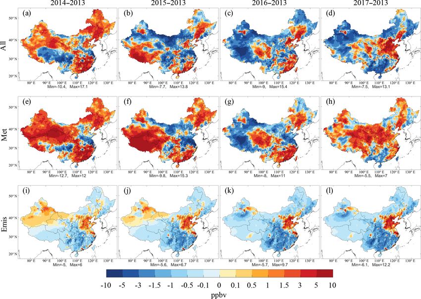
6306                          Y. Liu and T. Wang: Worsening urban ozone pollution in China from 2013 to 2017 – Part 1

major urban areas of China have continued to increase, and        and showed that four meteorological factors, including tem-
the magnitude and frequency of high-ozone events are much         perature, relative humidity, etc., accounted for 76 % of the
greater in China than in cities in Japan, South Korea, Europe,    variability in the baseline ozone level. P. F. Wang et al. (2019)
and the United States (Lu et al., 2018). The ozone problem        used a chemistry transport model (Community Multiscale
has become a new challenge to air quality management in           Air Quality modeling system; CMAQ) to investigate the re-
China. A comprehensive understanding of the causes of the         sponse of summer ozone concentrations to changes in mete-
increase in surface ozone levels in China is necessary to de-     orological conditions from 2013 to 2015, and they showed
velop a comprehensive whole-air improvement strategy.             that the maximum daily 8 h average (MDA8) O3 mixing ra-
   Ground-level ozone is produced in situ by chemical re-         tio decreased by 5 to 10 ppb in most cities due to changes in
actions from ozone precursors, NOx , volatile organic com-        meteorological conditions and biogenic emissions in the lat-
pounds (VOCs), and carbon monoxide (CO) or transported            ter 2 years, except for some cities in eastern, south-central,
from outside the region and from higher altitudes (Atkinson,      and southwestern China in which the ozone mixing ratio in-
2000; Roelofs and Lelieveld, 1997; Akimoto et al., 2015).         creased by less than 10 ppb. Lu et al. (2019a) used the GEOS-
Meteorological conditions affect the surface ozone concen-        Chem model to explore changes in source attributions con-
trations directly via changes in chemical reaction rates, di-     tributing to ozone changes over China in 2016 and 2017 and
lution, wet and dry removal, and transport flux or indirectly     suggested that the increases in ozone in 2017 relative to 2016
via changes in natural emissions (Lu et al., 2019b; Lin et        were mainly caused by higher background ozone driven by
al., 2008). As for the direct effects, an increase in tempera-    hotter and drier weather conditions.
ture can enhance ozone formation by altering the chemical            Despite these studies, a more comprehensive understand-
reaction rates (Lee et al., 2014; Fu et al., 2015), and an in-    ing of the role of the meteorological conditions in the recent
crease in water vapor can lead to a decrease in ozone con-        ozone changes is still warranted. Previous analyses with a
centrations in the lower troposphere (Kalabokas et al., 2015;     statistical method have been limited to a few cities (i.e., Bei-
He et al., 2017). An increase in the planetary boundary layer     jing and Guangzhou). China has a vast territory with a wide
(PBL) height can decrease ozone levels via dilution of pri-       range of climates, so the meteorological conditions in vari-
mary pollutants into a larger volume of air (Sanchez-Ccoyllo      ous parts of China may have experienced different changes
et al., 2006). Clouds have also been shown to decrease ozone      in recent years. Previous chemical transport modeling studies
concentrations via aqueous-phase chemistry and photochem-         examined either the meteorological impact for 2 or 3 years
istry, which enhances scavenging of oxidants and reduces the      (no more), the combined (not individual) effects of meteoro-
oxidative capacity of the troposphere (Lelieveld and Crutzen,     logical parameters, or the combined (not separate) effect of
1990), and precipitation decreases the ozone concentration        biogenic emission and meteorology changes.
via the wet removal of ozone precursors (Seinfeld and Pan-           The objective of our study is to investigate the effects
dis, 2006; Shan et al., 2008). Wind fields can significantly      of changes in meteorological conditions and anthropogenic
affect ozone by transporting ozone and ozone precursors in        emissions on summer surface ozone increases over China
and out of the region of interest (Lu et al., 2019a; Sanchez-     from 2013 to 2017 using an up-to-date regional chemical
Ccoyllo et al., 2006). As for the indirect effects, an increase   transport model driven by the interannual meteorological
in temperature can enhance the biogenic emissions of VOCs         conditions and anthropogenic emissions over the 5 years.
and thus affect ozone production (Tarvainen et al., 2005;         This paper (Part 1) assesses the role of meteorological con-
Guenther et al., 2006; Im et al., 2011).                          ditions, and a companion paper (Part 2; Liu and Wang,
   Several studies have used statistical analysis or numerical    2020) focuses on the role of anthropogenic emissions and
modeling to assess the effects of meteorological variations       implications for multi-pollutant control. Section 2 introduces
on the recent urban ozone trend in China. Using a conver-         the observational data, the model used, and experiment set-
gent cross-mapping method to overcome the interactions be-        tings. In Sect. 3, we first evaluate the simulated meteoro-
tween various factors, Chen et al. (2019) quantified the influ-   logical factors and pollutant concentrations based on the
ence of individual meteorological factors on the O3 concen-       observations. Subsequently, we separate the changes in the
tration in Beijing from 2006 to 2016. The results indicated       MDA8 O3 due to the variations in meteorological conditions
that temperature was the critical meteorological driver of the    and anthropogenic emissions by conducting numerical sen-
summer ozone concentrations in Beijing. Cheng et al. (2019)       sitivity experiments and explore their contributions to the
applied the Kolmogorov–Zurbenko filtering method to the           ozone changes during the 5 years. Considering the impor-
ozone variations in Beijing from 2006 to 2017, and the re-        tance of biogenic emissions to ozone production, we esti-
sults suggested that the relative contribution of meteorologi-    mate the meteorology-driven biogenic emissions over China
cal conditions to long-term variation in ozone was only 2 %       from 2013 to 2017 and assess their impacts on the variations
to 3 %, but short-term ozone concentrations were affected         in ozone. Lastly, the effects of changes in individual mete-
significantly by variations in meteorological conditions. Yin     orological factors are examined, and the role of long-range
et al. (2019) also used the Kolmogorov–Zurbenko approach          transport is assessed. Section 4 summarizes the conclusions.
to analyze the ozone data for Guangzhou from 2014 to 2018

Atmos. Chem. Phys., 20, 6305–6321, 2020                                             https://doi.org/10.5194/acp-20-6305-2020
Y. Liu and T. Wang: Worsening urban ozone pollution in China from 2013 to 2017 – Part 1                                   6307

2     Methods                                                     modeling domain to reduce the effect of the meteorologi-
                                                                  cal boundary from the WRF model, covers all the land areas
2.1    Measurement data                                           of China and the surrounding regions. The boundary con-
                                                                  ditions of chemical species for CMAQ were derived from
We used observational data to evaluate the meteorological         the modeling results of the global chemistry transport model,
parameters and air pollutant concentrations simulated by the      Model for Ozone and Related Chemical Tracers, version 4
Weather Research and Forecasting (WRF)-CMAQ model.                (MOZART-4) (http://www.acom.ucar.edu/wrf-chem/mozart.
The daily meteorological observations were obtained from          shtml, last access: 1 December 2019) (Emmons et al., 2010).
the National Meteorological Information Center (http://data.      We used SAPRC07TIC (Carter, 2010; Hutzell et al., 2012;
cma.cn, last access: 1 December 2019), including the daily        Xie et al., 2013; Lin et al., 2013) as the gas-phase chemi-
average temperature at a height of 2 m, relative humidity at      cal mechanism and AERO6i (Murphy et al., 2017; Pye et al.,
a height of 2 m, wind speed at a height of 10 m, and surface      2017) as the aerosol mechanism in the CMAQ model.
pressure at ∼ 700 ground weather stations in China. The ob-          The original CMAQ model includes the heterogeneous re-
served concentrations of air pollutants were obtained from        actions of only NO2 , NO3 , and N2 O5 on aerosol surfaces.
the China National Environmental Monitoring Center (http:         Recent studies (K. Li et al., 2019a, b) have suggested that
//106.37.208.233:20035/, last access: 1 December 2019), in-       the heterogeneous reactions on aerosol surfaces, mainly the
cluding SO2 , NO2 , CO, O3 , and PM2.5 . In 2013, there were      uptake of HO2 , played a significant role in the increasing O3
493 environmental monitoring stations in 74 major cities,         concentrations in China from 2013 to 2017. To better simu-
mostly in urban areas. As a result, only these stations have      late the effects of aerosol on ozone via heterogeneous reac-
continuous 5-year observations of pollutants from 2013 to         tions, we updated the heterogeneous reaction rates of NO2
2017. With the increasing recognition of the air pollution        and NO3 on the aerosol surface and incorporated more het-
problem in China, more monitoring stations have been built        erogeneous reactions into the CMAQ model, including the
since 2013, and the total number exceeded 1500 in 2017. We        uptake of HO2 , O3 , OH, and H2 O2 . The detailed heteroge-
applied data quality control to the observed pollutant concen-    neous reactions in the updated CMAQ model are listed in
trations to remove unreliable outliers following the approach     Table S2. We select the “best guess” uptake coefficients of
used in previous studies (Lu et al., 2018; Song et al., 2017).    these gases, which have been widely used in previous chem-
The locations of environmental monitoring stations are pre-       ical transport model studies (Jacob, 2000; Zhu et al., 2010;
sented in Fig. S1 in the Supplement.                              Zhang and Carmichael, 1999; Fu et al., 2019; Liao et al.,
   To evaluate the model performance, we calculated some          2004). These improvements help the CMAQ model better
statistical parameters, including the mean observation, mean      simulate ozone and other pollutants, and their influence and
simulation, mean bias, mean absolute gross error, root mean       that of aerosol on the ozone concentration via various het-
square error, index of agreement, and correlation coefficient.    erogeneous reactions are evaluated in the companion paper
The equations for these statistical parameters can be found in    (Part 2; Liu and Wang, 2020).
Fan et al. (2013).
                                                                  2.3   Emissions
2.2    Model settings
                                                                  For anthropogenic emissions, we used the Multi-resolution
The CMAQ modeling system (Byun and Schere, 2006) was              Emission Inventory for China (MEIC) for 2013 to 2017
developed by the United States Environmental Protection           (http://www.meicmodel.org/, last access: 1 December 2019),
Agency (US EPA) to approach air quality as a whole by             which was developed by Tsinghua University and has been
including state-of-the-art capabilities to model multiple air     evaluated by satellite data and ground observations (Zheng
quality issues, including tropospheric ozone, fine particles,     et al., 2018). International shipping emissions in 2010 were
toxins, acid deposition, and visibility degradation. This study   obtained from the Hemispheric Transport Atmospheric Pol-
used the CMAQ model (version 5.2.1), an offline chemical          lution emissions version 2.0 dataset (Janssens-Maenhout et
transport model without considering the effects of air pol-       al., 2015). Biogenic emissions from 2013 to 2017 were cal-
lutants on meteorological fields. The meteorological inputs       culated from the Model of Emissions of Gases and Aerosols
are driven by the WRF model. Table S1 in the Supplement           from Nature (MEGAN) (Guenther et al., 2006) and driven by
shows the settings of the physical parameterization schemes       the interannual summer meteorological inputs from the WRF
for the WRF model. The meteorological initial and bound-          model.
ary conditions were provided by NCEP/NCAR FNL reanal-
ysis data with a horizontal resolution of 1◦ . Figure S1 shows    2.4   Experiment settings
the modeling domains for the WRF and CMAQ model with
a horizontal resolution of 36 km. The model has 23 verti-         The model simulations were conducted for the summers
cal layers and reaches 50 hPa at the top. The CMAQ mod-           (June, July, and August) from 2013 to 2017 and driven by in-
eling domain, which is a few grids smaller than the WRF           terannual meteorology and anthropogenic emissions, namely

https://doi.org/10.5194/acp-20-6305-2020                                            Atmos. Chem. Phys., 20, 6305–6321, 2020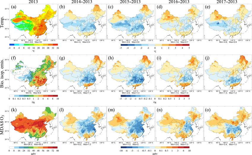
6308 Y. Liu and T. Wang: Worsening urban ozone pollution in China from 2013 to 2017 – Part 1
the base simulations. The shipping emissions remained un- of 2 m decreased from 2013 to 2015 and then increased from
changed in the 5-year simulation due to a lack of data for re- 2015 to 2017, which is consistent with the observations. The
cent years. To investigate the causes of the increasing surface good performance of the WRF model gives us the confidence
ozone levels in China, we conducted four sets of modeling to use the simulations to study the effects of variations in me-
experiments based on the simulation of 2013. The first was teorological conditions on ozone levels.
designed to evaluate the effects of changes in meteorologi- Table 2 presents the evaluation results for air pollutant
cal conditions and anthropogenic emissions (Table S3). We concentrations in China. Generally, the CMAQ model has ex-
derived the effects of meteorological variation by compar- cellent performance on simulating pollutant concentrations
ing the simulated ozone concentrations in different years but with low biases, high index of agreement, and high cor-
with the same anthropogenic emissions and chemical bound- relation coefficients. The simulated NO2 mixing ratio was
ary conditions as those from 2013. The effects of changes slightly underestimated for these 5 years in general, which
in anthropogenic emissions were derived by comparing the can be explained in part by the fact that the NO2 concen-
simulated ozone values in 2013 but with anthropogenic emis- trations in the national network were measured using the
sions from different years. The second set was designed to catalytic conversion method, which overestimates NO2 , es-
evaluate the effects of variations in biogenic emissions driven pecially during periods with active photochemistry and at
by meteorological conditions (Table S4), which were derived locations away from primary emission sources (Xu et al.,
by comparing the simulated ozone values in 2013 but with 2013; Zhang et al., 2017; Fu et al., 2019). The simulated CO
biogenic emissions from different years. The third set was mixing ratio is underestimated significantly by the CMAQ
designed to evaluate the contributions of the individual me- model, which might be due to the missing sources of CO such
teorological parameters to the ozone change from 2013 to as biomass burning. The CMAQ model predicts a slightly
2017 (Table S5), including temperature, specific humidity, higher MDA8 O3 mixing ratio, which could be explained by
wind field, PBL height, clouds, and precipitation. Here we the artificial mixing of ozone precursors in modeling grids
used specific humidity rather than relative humidity, because leading to higher ozone production efficiency and positive
the specific humidity, which scaled with water vapor concen- ozone biases, especially for models with coarser resolutions
trations and was simulated by the model, was more useful (Young et al., 2018; Chen et al., 2018; Yu et al., 2016). How-
for understanding the ozone formation chemistry. The fourth ever, the overall CMAQ model performance is acceptable
set (Table S6) was designed to evaluate the contribution of and can support further investigation of the drivers of increas-
long-range transport from outside the CMAQ modeling do- ing ozone levels in China.
main (Fig. S1) by comparing the simulated ozone levels in
2013 with those with chemical boundary conditions from 3.2 Rate of change in ozone due to meteorology and
MOZART from different years. anthropogenic emission
Figure 1 shows the spatial distribution of the summer surface
3 Results MDA8 O3 level over land areas of China in summer from
2013 to 2017. The CMAQ model can faithfully capture the
3.1 Model evaluation spatiotemporal variations in the observed MDA8 O3 level.
Both the simulations and the observations exhibit elevated
Table 1 shows the evaluation results for temperature, relative concentration in midlatitude areas, including the North China
humidity, wind speed, and surface pressure. The results for Plain (NCP), Yangtze River Delta (YRD), Sichuan Basin
all weather stations in China were averaged. The simulated (SCB), and large areas in central and western China. The
temperatures at the height of 2 m were slightly underesti- O3 levels in southern China are lower than those in northern
mated with biases of less than 0.6 ◦ C in 5 years. The high cor- China, but they are relatively high in the Pearl River Delta
relation coefficients (over 0.82) indicate that the WRF model (PRD) region.
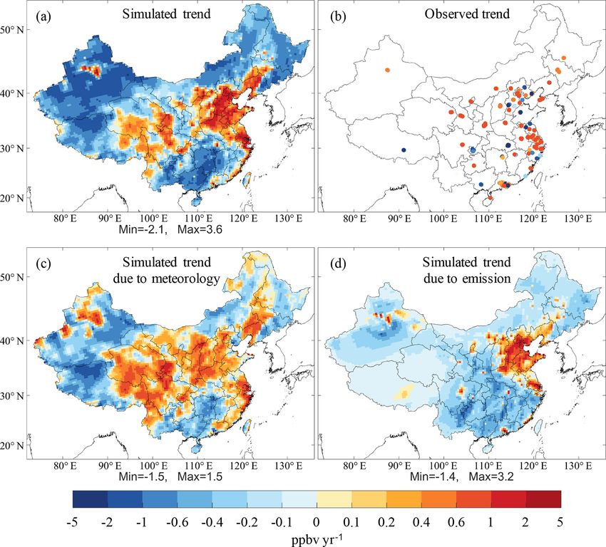
can capture variations in temperature. Like temperature, the We applied the linear regression method to obtain rates of
simulated relative humidity values were also slightly under- change in the simulated and observed interannual MDA8 O3 ,
predicted and had a high correlation coefficient with the ob- which are shown in Fig. 2. In general, the observed MDA8
servations. The simulated wind speeds at the height of 10 m O3 mixing ratios present an increasing trend from 2013 to
were slightly overestimated by about 0.5 m s−1 due to the un- 2017 in many of the 493 monitoring stations (most located in
derestimation of the effects of urban topography in the WRF urban areas of 74 major cities), while the trend result at some
model and were often found in other WRF modeling studies of these sites has relatively low confidence level as indicated
(Fan et al., 2015; Hu et al., 2016). The WRF model faith- by large p values (Fig. S2). The model captured 57 % of the
fully reproduces surface pressures for 5 years with low biases observed rate of increase averaged for the 493 sites (Fig. S3).
and high correlation coefficients. The WRF model could also With the aid of the model simulations, the characteristics of
capture the temporal variations in meteorological parame- the changes in MDA8 O3 levels were revealed for all areas,
ters. For example, the simulated temperature at the height including those with no monitoring stations. Both observa-
Atmos. Chem. Phys., 20, 6305–6321, 2020 https://doi.org/10.5194/acp-20-6305-2020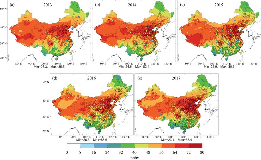
Y. Liu and T. Wang: Worsening urban ozone pollution in China from 2013 to 2017 – Part 1                                                 6309

Table 1. Evaluation results for the meteorological factors (T2 is temperature at a height of 2 m; RH2 is relative humidity at a height of 2 m;
WS10 is wind speed at a height of 10 m; PRS is surface pressure; Num is number of sites with available observation for statistics; OBS is
mean observation; SIM is mean simulation; MB is mean bias; MAGE is mean absolute gross error; RMSE is root mean square error; IOA is
index of agreement; r is correlation coefficient; OBS, SIM, MB, MAGE, and RMSE have the same units as given in the first column, while
IOA and r have no unit).

                          Species    Year    Num       OBS      SIM        MB     MAGE       RMSE      IOA        r
                          T2         2013      692     23.9     23.3     −0.6         2.1       2.3    0.99    0.82
                          (◦ C)      2014      690     23.1     22.8     −0.3         1.9       2.2    0.99    0.82
                                     2015      708     23.0     22.5     −0.5         1.9       2.2    0.99    0.83
                                     2016      694     23.8     23.2     −0.6         2.0       2.3    0.99    0.82
                                     2017      694     23.7     23.2     −0.5         2.0       2.2    0.99    0.86
                          RH2        2013      692     70.5     67.6     −2.9        10.1      11.9    0.99    0.72
                          (%)        2014      690     72.2     67.2     −5.0        10.1      11.9    0.99    0.68
                                     2015      708     71.2     67.6     −3.6         9.2      10.9    0.99    0.72
                                     2016      694     72.0     68.4     −3.6         9.2      10.9    0.99    0.71
                                     2017      694     71.7     67.7     −4.1         9.4      11.1    0.99    0.73
                          WS10       2013      692      2.1       2.8      0.7        1.0       1.2    0.93    0.53
                          (m s−1 )   2014      690      1.9       2.5      0.5        0.9       1.0    0.94    0.47
                                     2015      708      2.1       2.6      0.6        0.9       1.1    0.94    0.54
                                     2016      694      2.1       2.6      0.5        0.9       1.1    0.94    0.50
                                     2017      694      2.1       2.6      0.5        0.9       1.1    0.94    0.49
                          PRS        2013      692    922.4    906.2    −16.2        21.0      21.0    0.99    0.98
                          (hPa)      2014      690    924.0    907.8    −16.3        21.1      21.1    0.99    0.98
                                     2015      708    924.0    907.9    −16.1        21.1      21.1    0.99    0.97
                                     2016      694    923.4    907.5    −15.9        20.7      20.7    0.99    0.98
                                     2017      694    923.4    907.8    −15.6        20.5      20.6    0.99    0.98

tions and model simulations show that NCP, YRD, SCB,                     A recent study reported the observations of surface ozone
northeastern China, and some areas in western China experi-              during 1994–2018 at a coastal site in southern China and re-
enced increasing levels of ozone pollution. Interestingly, the           vealed no significant changes in the ozone levels in the out-
model results revealed that MDA8 O3 levels were decreasing               flow of air masses from mainland China during recent years
in large parts of rural areas that could not be covered by the           (T. Wang et al., 2019). These results suggest that nationwide
current monitoring stations, such as northwestern China and              NOx emission reductions may have decreased ozone produc-
southern China.                                                          tion over large regions despite causing an ozone increase in
   We separated the changing rates of simulated MDA8 O3                  urban areas. The impact of anthropogenic emission changes
into those due to variations in meteorological conditions                on ozone levels in recent years remains a challenging and
and changes in anthropogenic emissions (also see Fig. 2).                momentous topic and will be assessed in the companion pa-
Here, the impact of biogenic emission variation is included              per (Part 2; Liu and Wang, 2020). The present paper focuses
in the effects of meteorological variation, because it is af-            on the effects of meteorological conditions.
fected by meteorology. The result shows that the changing
rates of ozone over China were more affected by meteoro-                 3.3     Impact of meteorological conditions and
logical changes than by emission changes in terms of spa-                        anthropogenic emissions relative to 2013
tial distribution. The regions with an increasing or decreasing
trend of ozone were generally consistent with the contribu-              We next quantified the impact of meteorological conditions
tions from variations in meteorology except for some regions             and anthropogenic emissions on ozone changes from 2013
whose ozone trends were dominated by anthropogenic emis-                 to 2017 relative to 2013 (Fig. 3). The changes in MDA8
sion changes. The changes in anthropogenic emissions have                O3 from the base simulation varied spatially and yearly,
resulted in ozone increases in NCP, YRD, PRD, SCB, and                   mainly as a result of meteorological conditions. The vari-
other scattered megacities but decreases in rural regions. This          ation in the MDA8 O3 mixing ratio due to meteorological
discrepancy can be explained by the different ozone forma-               changes ranged from −12.7 to 15.3 ppbv over China from
tion regimes in urban (VOCs-limited) areas and rural (NOx -              2014 to 2017 relative to 2013. The emission-induced MDA8
limited) areas (K. Li et al., 2019a; N. Wang et al., 2019).              O3 changes in each year exhibited similar spatial patterns,
                                                                         which were consistent with those of the changing rates due to

https://doi.org/10.5194/acp-20-6305-2020                                                    Atmos. Chem. Phys., 20, 6305–6321, 2020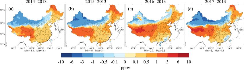
6310                              Y. Liu and T. Wang: Worsening urban ozone pollution in China from 2013 to 2017 – Part 1

Table 2. Evaluation results for the air pollutants in China (Num is number of sites with available observation for statistics; OBS is mean
observation; SIM is mean simulation; MB is mean bias; MAGE is mean absolute gross error; RMSE is root mean square error; IOA is index
of agreement; r is correlation coefficient; OBS, SIM, MB, MAGE, and RMSE have the same units as given in the first column, while IOA
and r have no unit).

                         Species       Year    Num     OBS     SIM       MB     MAGE       RMSE      IOA       r
                         SO2           2013     408     7.1    12.0      4.9        7.6       9.1    0.79   0.28
                         (ppbv)        2014     867     6.4     9.0      2.6        5.9       7.0    0.80   0.26
                                       2015    1410     5.0     5.2      0.2        4.0       4.8    0.77   0.23
                                       2016    1422     4.4     4.1     −0.3        3.4       4.0    0.77   0.24
                                       2017    1474     3.8     3.2     −0.6        2.7       3.1    0.77   0.22
                         NO2           2013     430    15.1    16.6      1.4        7.0       8.3    0.91   0.41
                         (ppbv)        2014     843    13.9    13.8     −0.1        6.6       7.7    0.89   0.37
                                       2015    1411    11.3     9.9     −1.4        5.7       6.7    0.84   0.34
                                       2016    1420    10.9     9.5     −1.4        5.5       6.4    0.85   0.35
                                       2017    1480    11.3     9.5     −1.8        5.9       6.8    0.83   0.32
                         CO            2013     436    0.71    0.34   −0.37        0.39      0.45    0.81   0.33
                         (ppmv)        2014     872    0.75    0.32   −0.42        0.44      0.49    0.79   0.34
                                       2015    1400    0.65    0.28   −0.38        0.39      0.44    0.78   0.32
                                       2016    1419    0.65    0.26   −0.39        0.40      0.44    0.78   0.33
                                       2017    1473    0.62    0.25   −0.37        0.38      0.41    0.78   0.30
                         MDA8 O3       2013     371    50.9    57.7       6.8      17.8      21.3    0.95   0.55
                         (ppbv)        2014     836    52.5    59.2       6.7      17.7      21.1    0.95   0.54
                                       2015    1361    50.4    56.4       5.9      15.3      18.3    0.96   0.55
                                       2016    1373    52.3    57.6       5.3      13.4      16.3    0.97   0.61
                                       2017    1440    56.3    58.3       1.9      13.1      16.1    0.98   0.63
                         PM2.5         2013     437    44.4    42.8     −1.7       19.4      26.0    0.91   0.58
                         (µg m−3 )     2014     869    43.8    43.6     −0.2       19.1      24.5    0.92   0.57
                                       2015    1401    35.3    31.6     −3.7       16.4      20.6    0.89   0.54
                                       2016    1411    29.7    27.0     −2.7       13.5      17.0    0.90   0.54
                                       2017    1462    27.8    24.5     −3.3       12.6      15.8    0.89   0.52

emission changes (Fig. 2d). The impact of emission changes             anthropogenic emissions on ozone levels (Fig. 4) – Beijing,
on the MDA8 O3 concentrations became increasingly signif-              Shanghai, Guangzhou, and Chengdu – which are principal
icant as anthropogenic emissions were further reduced. Our             cities in the Beijing-Tianjin-Hebei (BTH) region in the north,
results differ from those by P. F. Wang et al. (2019), who sug-        the YRD in the east, the PRD in the south, and the SCB in the
gested a less important role of meteorology in the variation           southwestern part of China, respectively (see Fig. S1 for their
of ozone from 2013 to 2015. The discrepancy could be due to            locations). The numbers of monitoring sites used to obtain
the difference in the chemical mechanisms and method used              the average values for these four cities were 12, 9, 11, and 8,
for quantifying the effects of emission changes. They calcu-           respectively. Most of these sites are situated inside the city,
lated the changes in ozone levels due to emission variations           and thus the average results represent the conditions in urban
by subtracting simulated changes due to meteorological con-            areas. As shown in Fig. 4, the changes in observed MDA8
ditions variations from total observed changes, and we cal-            O3 varied in cities and years, which were generally captured
culated by comparing the simulated difference between the              by the model (except for the changes of MDA8 O3 in Beijing
simulations in 2013 driven by anthropogenic emissions from             in 2014 and 2015, which were underestimated, likely due to
different years.                                                       underestimation of anthropogenic emissions in Beijing and
   We further found that in some specific regions and years,           its surrounding regions in those 2 years). The contributions
the changes in MDA8 O3 due to meteorological variation                 of anthropogenic emissions to MDA8 O3 exhibited an almost
could be comparable to or greater than those due to emission           linear increasing trend in the four cities from 2013 to 2017,
changes, which highlights the significant role of meteorolog-          whereas the contribution of meteorology could be positive or
ical conditions in ozone variations. As a result, we selected          negative, depending on the region and year.
four megacities in different regions of China to further exam-            In Beijing (the BTH region), the variations in meteorologi-
ine the impact of changes in meteorological conditions and             cal conditions had little effect on the MDA8 O3 changes from

Atmos. Chem. Phys., 20, 6305–6321, 2020                                                   https://doi.org/10.5194/acp-20-6305-2020
Y. Liu and T. Wang: Worsening urban ozone pollution in China from 2013 to 2017 – Part 1 6311
Figure 1. Spatial distribution of the simulated surface maximum daily 8 h average (MDA8) O3 mixing ratios in summer (June–August) of
2013 (a), 2014 (b), 2015 (c), 2016 (d), and 2017 (e). Circles with color are the available observed values at environmental monitoring stations
in each year.
2014 to 2017 relative to 2013. The increase in ozone was Guangzhou from 2013 to 2015, both indicating meteorolog-
driven primarily by the changes in anthropogenic emissions. ical variations unfavorable for ozone formation in Shanghai
This characteristic can also be identified in the larger BTH and favorable in Guangzhou. On the other hand, our simu-
region, as shown in Fig. 3. In Shanghai (the YRD region), lations differ from theirs that showed a considerable nega-
the effects of meteorology were comparable with those of tive contribution of the meteorology variations to ozone lev-
anthropogenic emissions in terms of the absolute values of els in Beijing and Chengdu. Our study and that of Chen et
the contribution to MDA8 O3 changes. From 2014 to 2016, al. (2019) suggest a weak role of meteorology variation in
the meteorology was unfavorable for ozone formation, which the summer ozone trend in Beijing. In addition to these four
masks the ozone increase due to emission changes. How- regions, we found a significant impact of meteorology on
ever, meteorological conditions became a positive driver in the ozone change in western China, especially the Qinghai–
2017, leading to a drastic increase in the total MDA8 O3 Tibetan Plateau (Fig. 3). The meteorological variations con-
mixing ratio (over 10 ppb). In Guangzhou (the PRD region), tributed to considerable increases in MDA8 O3 in 2014–2017
the role of meteorological conditions was opposite to that in this region relative to 2013.
in Shanghai. The weather changes were conducive to ozone
formation from 2014 to 2016 compared with 2013, contribut- 3.4 Impact of meteorology-driven biogenic emissions
ing to a large increase in MDA8 O3 by over 10 ppbv; in relative to 2013
2017, however, the impact of changes in meteorological con-
ditions on ozone levels decreased substantially, leading to a Temperature is an important meteorological driver of bio-
moderate increase in MDA8 O3 in that year compared with genic emissions. Figure 5 displays the temperature changes
2013. In Chengdu (the SCB region), the impact of meteo- in land areas of China from 2014 to 2017 compared with
rological conditions on ozone variation was limited in these 2013. The changes in the spatial distribution were similar
years, and the ozone level was mainly affected by emission in these 4 years. A decrease in temperature was found in
changes, similar to the situation in Beijing. Our result is sim- midlatitude areas (25 to 40◦ N), and an increase was found
ilar to those by P. F. Wang et al. (2019) for Shanghai and in southern (south of 25◦ N) and northern China (north of
40◦ N). As shown in Fig. S4, in midlatitude areas such as the
https://doi.org/10.5194/acp-20-6305-2020 Atmos. Chem. Phys., 20, 6305–6321, 20206312 Y. Liu and T. Wang: Worsening urban ozone pollution in China from 2013 to 2017 – Part 1 Figure 2. Rates of changes in the simulated (a) and observed (b) surface MDA8 O3 mixing ratios in summer from 2013 to 2017. In panel (b), only environmental monitoring sites (493) with data available in all 5 years are presented. (c) and (d) present the rates of changes in the simulated MDA8 O3 mixing ratios due to variations in meteorological conditions and anthropogenic emissions in summer from 2013 to 2017 (see Methods section). The corresponding p values of regression are presented in Fig. S2. BTH, YRD, and SCB, the temperature decreased from 2013 east China, which have high vegetation covers in summer to 2015 and then increased from 2015 to 2017. In contrast, in (Fig. 5f). The spatial and interannual variations of biogenic southern China, such as the PRD region, the temperature in- isoprene emissions followed the changes in temperatures in creased during 2013–2014 and then slightly decreased during China, leading to similar changes in MDA8 O3 concentra- 2014–2017. The variation in the observed temperature is well tions. captured by the WRF model, which enables the MEGAN In midlatitude areas of China, the variations in biogenic model to calculate the variation of biogenic emissions driven emissions induced a decrease in the MDA8 O3 level af- by the realistic temperature. We present the results of bio- ter 2013. The most significant decrease in the MDA8 O3 genic isoprene emissions, because isoprene is generally the level was found in the YRD and SCB regions, where there most abundant biogenic VOC and has the highest ozone for- were high biogenic emissions and a drastic temperature de- mation potential (Zheng et al., 2009). Large isoprene emis- crease. In 2014 and 2015, the MDA8 O3 mixing ratio de- sions were found in the southern parts of China and north- creased by ∼ 5 ppbv in these two regions compared with Atmos. Chem. Phys., 20, 6305–6321, 2020 https://doi.org/10.5194/acp-20-6305-2020
Y. Liu and T. Wang: Worsening urban ozone pollution in China from 2013 to 2017 – Part 1                                          6313

Figure 3. Changes in the simulated summer surface MDA8 O3 mixing ratios from the base simulation (All, a–d); those due to variations in
meteorological conditions (Met, e–h); and anthropogenic emissions (Emis, i–l) in 2014, 2015, 2016, and 2017 relative to 2013.

2013. The changes in ozone were less affected by biogenic             tions in ozone levels in recent years. Previous studies also
emissions due to the lower biogenic emissions and smaller             demonstrated the significant role of temperature in the ozone
variation of temperature in the BTH region. In southern and           trend in China and other regions (Hsu, 2007; Jing et al.,
northern China, the increase in temperature and then bio-             2014; Lee et al., 2014). However, the role of meteorology is
genic emissions since 2013 led to an enhancement of the               complex and the changes in other meteorological factors can
MDA8 O3 mixing ratio by up to 1 to 2 ppbv (Fig. 5). In                counteract this effect. In Beijing and Chengdu, for example,
Guangzhou, for example, affected by temperature-dependent             the changes in ozone levels due to variations in meteorology
biogenic emissions, the MDA8 O3 increased by 0.8 ppbv                 were insignificant and could not reflect those caused by vari-
from 2013 to 2014 and then decreased slightly from 2014               ations in temperature-dependent biogenic emissions (Fig. 4).
to 2017 (Fig. S5).
   The changes in MDA8 O3 concentrations due to changes               3.5   Impact of individual meteorological parameters in
in biogenic emissions in Shanghai and Guangzhou (Fig. S5)                   2017 relative to 2013
generally matched the total changes in ozone levels due to
variations in meteorological conditions and provided a con-           Figure 6 shows the individual effects of changing tempera-
siderable contribution to them (Fig. 4). The variations in            ture, humidity, wind field, PBL height, clouds, and precip-
biogenic emissions were mostly affected by temperature. In            itation between 2017 and 2013 on the ozone level. Of all
Sect. 3.5, we also found that the changes in ozone levels             the meteorological parameters, the change in wind fields had
caused by temperature variations via altering chemical re-            the most significant impact on MDA8 O3 . It led to an in-
action rates had an even more significant impact than via             crease in MDA8 O3 mixing ratio in nearly all of China,
changing biogenic emissions in 2017 relative to 2013. As a            with a maximum of 9.1 ppbv (Fig. 6i). Notable increases in
result, temperature can play an important role in the varia-          MDA8 O3 in western and eastern China due to the change in
                                                                      wind fields were identified, which contributed significantly

https://doi.org/10.5194/acp-20-6305-2020                                               Atmos. Chem. Phys., 20, 6305–6321, 2020
6314 Y. Liu and T. Wang: Worsening urban ozone pollution in China from 2013 to 2017 – Part 1 Figure 4. Interannual changes in the simulated (SIM) and observed (OBS) summer surface MDA8 O3 mixing ratios and those due to variations in meteorological conditions (MET) and anthropogenic emissions (EMIS) in (a) Beijing, (b) Shanghai, (c) Guangzhou, and (d) Chengdu in 2013–2017 relative to 2013. Figure 5. The simulated daytime averaged temperature at a height of 2 m (Temp., a–e) and total biogenic isoprene emissions (Bio. isop. emis., f–j) in summer of 2013 from the base simulations and their changes in 2014, 2015, 2016, and 2017 relative to 2013. Panels (k)–(o) (MDA8 O3 ) show the simulated summer surface MDA8 O3 mixing ratios in 2013 from the base simulation and their changes due to variations in biogenic emissions in 2014, 2015, 2016, and 2017 relative to 2013. Atmos. Chem. Phys., 20, 6305–6321, 2020 https://doi.org/10.5194/acp-20-6305-2020
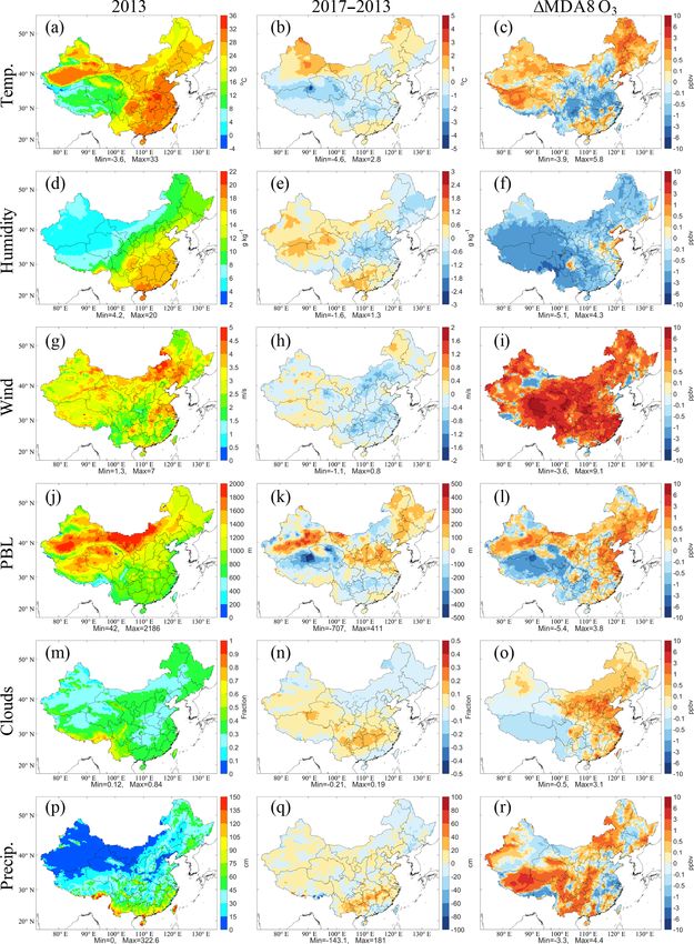
Y. Liu and T. Wang: Worsening urban ozone pollution in China from 2013 to 2017 – Part 1                                              6315

Figure 6. The simulated averaged temperature (Temp.) and specific humidity (Humidity) at a height of 2 m, wind speed at a height of 10 m
(Wind), planetary boundary layer (PBL) height, total clouds fraction (Clouds), and accumulated precipitation (Precip.) in the daytime in
summer of 2013 from the base simulation (the left column) and their changes in 2017 relative to 2013 (the central column). The right column
shows the changes in simulated summer surface MDA8 O3 mixing ratios due to variations in temperature, specific humidity, wind fields,
PBL height, clouds, and precipitation in 2017 relative to 2013.

https://doi.org/10.5194/acp-20-6305-2020                                                  Atmos. Chem. Phys., 20, 6305–6321, 2020
6316                           Y. Liu and T. Wang: Worsening urban ozone pollution in China from 2013 to 2017 – Part 1

to the meteorology-induced increasing ozone (Fig. 3h). In             The cloud fraction increased in southwestern China and
the Qinghai–Tibetan Plateau of western China, where terrain        the Qinghai–Tibetan Plateau but slightly decreased in other
heights are greater than 3 km, the significant increase in the     parts of China from 2013 to 2017 (Fig. 6n). Because clouds
MDA8 O3 mixing ratio (3 to 9 ppbv) due to wind change              can decrease ozone concentrations via aqueous-phase chem-
from 2013 to 2017 can be attributed in part to the enhanced        istry and photochemistry to enhance scavenging of oxi-
downward transport from the upper troposphere as indicated         dants and reduce the oxidative capacity of the troposphere
by the increase in the potential vorticity (PV) (Fig. S6). In      (Lelieveld and Crutzen, 1990), the MDA8 O3 mixing ratio in
eastern China, the increase in O3 level can be explained by        most parts of China increased except for southwestern China
the decrease in the wind speeds (Fig. 6h), which helps the ac-     and the Qinghai–Tibetan Plateau (Fig. 6o).
cumulation of O3 and its precursors and then increases ozone          The change in precipitation was similar to that of the cloud
concentrations. There is no strong evidence for the change in      fraction in terms of spatial distribution (Fig. 6q) but made an
the vertical transport from the free troposphere to the sur-       opposite contribution to ozone levels compared with clouds
face in eastern China and the horizontal transport from other      (Fig. 6r). A positive correlation (p = 0.95) between ozone
regions within the modeling domain between these 2 years,          and precipitation was also reported by the statistical results of
according to the wind data (Fig. S7).                              R. Li et al.(2019). Although precipitation can decrease ozone
   In addition to wind fields, other meteorological parame-        concentrations via the scavenging of ozone precursors (Se-
ters contribute to the ozone change. Because a high temper-        infeld and Pandis, 2006; Shan et al., 2008), an increase in
ature facilitates the formation of ozone via the increase in       precipitation may decrease aerosol concentrations that could
chemical reaction rates, the changes in ozone due to tem-          increase ozone levels by altering photolysis rates and hetero-
perature were consistent with the changes in temperature in        geneous reactions.
terms of spatial distribution (Fig. 6b and c). The MDA8 O3            The meteorological parameters that dominate ozone
decreased in central China and increased in other parts of         changes can differ in the four megacities (Fig. S9). The de-
China. This change in the spatial distribution was similar         crease in cloud cover was the important meteorological cause
to that due to the changes in biogenic emissions, because          that increased MDA8 O3 in Beijing from 2013 to 2017, the
they were both affected by temperature. However, comparing         wind field change was the dominant factor that increased and
Fig. 5o to Fig. 6c, we found that the impact of temperature        decreased the MDA8 O3 level in Shanghai and Guangzhou,
via the change in the chemical reaction rates was generally        respectively, and the decrease in temperature contributed pri-
more significant than that via the change in biogenic emis-        marily to the decline in MDA8 O3 in Chengdu. However,
sions from 2013 to 2017 (also see Fig. S8 for the quantitative     the effect of the dominant meteorological factor on variations
comparisons in different cities).                                  in the ozone level could be counteracted by the influence of
   The specific humidity decreased in central China and            other meteorological factors. For example, in Shanghai, the
northeast China but increased in other parts of China from         significant positive effect of changes in wind fields on ozone
2013 to 2017 (Fig. 6e). A decrease in the specific humidity        formation was offset by the negative effects of changes in
in central China led to an increase in the MDA8 O3 con-            temperature and precipitation, leading to the smaller increase
centration in localized areas, and an increase in other parts      in the ozone level due to the overall meteorological changes
of China resulted in a decrease in the MDA8 O3 concen-             in 2017 compared with 2013 (Fig. 6b). The synergistic or
tration in a large area (Fig. 6f). A negative correlation be-      counteracting effects from individual meteorological factors
tween ozone concentration and humidity in various regions          can give rise to the complex impact of the overall meteorol-
over China was also reported in many previous studies (Ma          ogy on ozone variations.
et al., 2019; R. Li et al., 2019).
   From 2013 to 2017, the PBL height increased in most parts       3.6   Impact of long-range transport relative to 2013
of China, including NCP, northeast China, and northwest
China (Fig. 6k). Our modeling results show that the increase       The chemical boundary conditions for the CMAQ model
in the PBL height enhanced the MDA8 O3 concentration in            were derived from the results of the MOZART global model,
most parts of China (Fig. 6l). A positive correlation between      which can represent the long-range transport of ozone and
the PBL height and the ozone level in China is also revealed       its precursors from outside the CMAQ modeling domain to
in the statistical results of He et al. (2017). Possible reasons   China and surrounding regions (Fig. S1). We changed the
for the ozone increase with the increase in the PBL height         chemical boundary conditions in 2013 to different years to
include lower NO concentration at the urban surface due to         investigate the role of long-range transport in ozone varia-
the deep vertical mixing, which then limits ozone destruc-         tions in China, and the results are shown in Fig. 7. Changes
tion and increases ozone concentrations (He et al., 2017), and     in long-range transport after 2013 increased the MDA8 O3
more downward transport of ozone from the free troposphere         mixing ratio over China except for some areas in northwest-
where the ozone concentration is higher than the near-surface      ern China. Compared with a small increase in MDA8 O3
concentration (Sun et al., 2010).                                  (< 1 ppbv) in eastern China, the Qinghai–Tibetan Plateau en-
                                                                   countered a significant increase in MDA8 O3 by about 1 to

Atmos. Chem. Phys., 20, 6305–6321, 2020                                              https://doi.org/10.5194/acp-20-6305-2020
Y. Liu and T. Wang: Worsening urban ozone pollution in China from 2013 to 2017 – Part 1 6317
Figure 7. Changes in the simulated summer surface MDA8 O3 mixing ratios due to variations in long-range transport in 2014, 2015, 2016,
and 2017 relative to 2013.
4 ppbv due to changes in long-range transport after 2013. In- and the changes in anthropogenic emissions dominated
creases in ozone levels were also found if we compared the the increase in ozone. Decreasing cloud cover was the
changes in MDA8 O3 due to variations in chemical bound- dominant meteorological factor that contributed to the
ary conditions relative to 2014. Ozone and its precursors can increase in MDA8 O3 .
be transported a long distance and then affect surface O3
in remote regions (West et al., 2009; Wild et al., 2004). A 2. In Shanghai (the Yangtze River Delta region), meteoro-
previous MOZART study by Li et al. (2014) found that the logical variation decreased ozone formation from 2014
transport from the emissions of all Eurasian regions except to 2016, which masked a large increase in ozone due to
China contributed 10 to 15 ppbv to the surface O3 mixing changes in emissions. The meteorological conditions in
ratio over western China. An analysis of 10 d back trajecto- 2017 became a positive driver for an increase in ozone,
ries at Mount Waliguan (a remote mountain site in western leading to a drastic increase in the total MDA8 O3 mix-
China) also showed that the air mass from central Asia con- ing ratio (over 10 ppb). Changes in biogenic emissions
tributed to the high O3 levels observed at the site during sum- had a significant impact on the ozone level in this re-
mer via long-range transport in the free troposphere (Wang et gion. The temperature decrease after 2013 resulted in a
al., 2006). Our study indicates a considerable increase (1 to considerable decline in MDA8 O3 , especially in 2014
4 ppbv) in this long-range transport contribution since 2013. and 2015. The wind field change was the dominant fac-
tor that increased MDA8 O3 in 2017 relative to 2013.
3. In Chengdu (the Sichuan Basin region), the impact of
4 Conclusions meteorological conditions on changes in ozone was lim-
ited from 2013 to 2017, and the ozone concentration
This study explored the impact of changes in meteorological was mainly affected by emissions, as in Beijing. How-
conditions and anthropogenic emissions on the recent ozone ever, the biogenic emissions induced by meteorologi-
variations across China. The changes in anthropogenic emis- cal conditions were important and led to a moderate de-
sions since 2013 increased the MDA8 O3 levels in urban ar- crease in the ozone level. The drop in temperature con-
eas but decreased the ozone levels in rural areas. The meteo- tributed to the decrease in MDA8 O3 in 2017 relative to
rological impact on the ozone trend varied by region and by 2013.
year and could be comparable with or even larger than the
impact of changes in anthropogenic emissions. The individ- 4. In Guangzhou (the Pearl River Delta region), the meteo-
ual effects of changes in temperature, specific humidity, wind rological conditions were more conducive to ozone for-
field, planetary boundary layer height, clouds, and precipita- mation from 2014 to 2016 than in 2013, which led to a
tion from 2013 to 2017 on the ozone levels were examined significant increase (> 10 ppbv) in MDA8 O3 . In 2017,
in this study. The results show that the changes in the wind the impact of changes in meteorological conditions on
fields made a significant contribution to the increase in sur- ozone levels decreased substantially, and the increase in
face ozone levels over many parts of China. The main find- MDA8 O3 was small and only due to the changes in
ings for various regions of China are summarized as follows. emissions. The biogenic emissions driven by meteoro-
logical conditions were also important to ozone forma-
1. In Beijing (the Beijing-Tianjin-Hebei region), the con- tion and increased MDA8 O3 after 2013. The wind field
tribution of meteorological changes to the variations in change was the dominant meteorological factor that de-
summer ozone was small in 2014–2017 relative to 2013, creased MDA8 O3 in 2017 compared with 2013.
https://doi.org/10.5194/acp-20-6305-2020 Atmos. Chem. Phys., 20, 6305–6321, 20206318 Y. Liu and T. Wang: Worsening urban ozone pollution in China from 2013 to 2017 – Part 1
5. In western China, the increase in ozone concentra- References
tions was mainly caused by meteorological conditions.
The increase in MDA8 O3 in Qinghai–Tibetan Plateau Akimoto, H., Mori, Y., Sasaki, K., Nakanishi, H., Ohizumi, T., and
from 2013 to 2017 was ascribed to enhanced down- Itano, Y.: Analysis of monitoring data of ground-level ozone in
Japan for long-term trend during 1990–2010: Causes of tem-
ward transport from the upper troposphere. The long-
poral and spatial variation, Atmos. Environ., 102, 302–310,
range transport of ozone and its precursors from outside https://doi.org/10.1016/j.atmosenv.2014.12.001, 2015.
the modeling domain also contributed to the increase Atkinson, R.: Atmospheric chemistry of VOCs and NOx , At-
in MDA8 O3 in most parts of China, especially on the mos. Environ., 34, 2063–2101, https://doi.org/10.1016/S1352-
Qinghai–Tibetan Plateau. 2310(99)00460-4, 2000.
Byun, D. and Schere, K. L.: Review of the governing equations,
In conclusion, our study highlights the complex but varying computational algorithms, and other components of the models-
effects of meteorological conditions on surface ozone levels 3 Community Multiscale Air Quality (CMAQ) modeling system,
across the regions of China and for different years. It is there- Appl. Mech. Rev., 59, 51–77, https://doi.org/10.1115/1.2128636,
2006.
fore necessary to consider meteorological variability when
Carter, W. P. L.: Development of the SAPRC-07 chem-
assessing the effectiveness of emission-control policies on
ical mechanism, Atmos. Environ., 44, 5324–5335,
changes in the levels of ozone (and other air pollutants) in https://doi.org/10.1016/j.atmosenv.2010.01.026, 2010.
different cities and/or regions of China. Such an approach Chen, X. Y., Liu, Y. M., Lai, A. Q., Han, S. S., Fan,
could be useful for the development of future air pollution Q., Wang, X. M., Ling, Z. H., Huang, F. X., and Fan,
mitigation policies. S. J.: Factors dominating 3-dimensional ozone distribution
tropospheric ozone period, Environ. Pollut., 232, 55–64,
https://doi.org/10.1016/j.envpol.2017.09.017, 2018.
Code and data availability. The code or data used in this study are Chen, Z., Zhuang, Y., Xie, X., Chen, D., Cheng, N., Yang,
available upon request from Yiming Liu (yming.liu@polyu.edu.hk) L., and Li, R.: Understanding long-term variations of me-
and Tao Wang (cetwang@polyu.edu.hk). teorological influences on ground ozone concentrations in
Beijing During 2006–2016, Environ. Pollut., 245, 29–37,
https://doi.org/10.1016/j.envpol.2018.10.117, 2019.
Supplement. The supplement related to this article is available on- Cheng, N. L., Li, R. Y., Xu, C. X., Chen, Z. Y., Chen, D. L.,
line at: https://doi.org/10.5194/acp-20-6305-2020-supplement. Meng, F., Cheng, B. F., Ma, Z. Q., Zhuang, Y., He, B., and
Gao, B. B.: Ground ozone variations at an urban and a rural
station in Beijing from 2006 to 2017: Trend, meteorological
influences and formation regimes, J. Clean Prod., 235, 11–20,
Author contributions. TW initiated the research, YL and TW de-
https://doi.org/10.1016/j.jclepro.2019.06.204, 2019.
signed the paper framework. YL ran the model, processed the data,
Emmons, L. K., Walters, S., Hess, P. G., Lamarque, J.-F., Pfis-
and made the plots. YL and TW analyzed the results and wrote the
ter, G. G., Fillmore, D., Granier, C., Guenther, A., Kinnison,
paper.
D., Laepple, T., Orlando, J., Tie, X., Tyndall, G., Wiedinmyer,
C., Baughcum, S. L., and Kloster, S.: Description and eval-
uation of the Model for Ozone and Related chemical Trac-
Competing interests. The authors declare that they have no conflict ers, version 4 (MOZART-4), Geosci. Model Dev., 3, 43–67,
of interest. https://doi.org/10.5194/gmd-3-43-2010, 2010.
Fan, Q., Liu, Y. M., Wang, X. M., Fan, S. J., Chan, P.
W., Lan, J., and Feng, Y. R.: Effect of different meteo-
Acknowledgements. We would like to thank Qiang Zhang from Ts- rological fields on the regional air quality modelling over
inghua University for providing the emission inventory, Qi Fan from Pearl River Delta, China, Int. J. Environ. Pollut., 53, 3–23,
Sun Yat-sen University for helping to access the meteorological https://doi.org/10.1504/ijep.2013.058816, 2013.
data, Xiao Fu from The Hong Kong Polytechnic University for shar- Fan, Q., Lan, J., Liu, Y. M., Wang, X. M., Chan, P. W., Hong, Y.
ing the model codes of HONO sources. Y., Feng, Y. R., Liu, Y. X., Zeng, Y. J., and Liang, G. X.: Pro-
cess analysis of regional aerosol pollution during spring in the
Pearl River Delta region, China, Atmos. Environ., 122, 829–838,
Financial support. This research has been supported by the https://doi.org/10.1016/j.atmosenv.2015.09.013, 2015.
Hong Kong Research Grants Council (grant no. T24-504/17-N) Fleming, Z. L., Doherty, R. M., von Schneidemesser, E., Mal-
and the National Natural Science Foundation of China (grant ley, C. S., Cooper, O. R., Pinto, J. P., Colette, A., Xu, X.
no. 91844301). B., Simpson, D., Schultz, M. G., Lefohn, A. S., Hamad,
S., Moolla, R., Solberg, S., and Feng, Z. Z.: Tropospheric
Ozone Assessment Report: Present-day ozone distribution and
Review statement. This paper was edited by Jianzhong Ma and re- trends relevant to human health, Elementa-Sci. Anthrop., 6, 12,
viewed by two anonymous referees. https://doi.org/10.1525/elementa.273, 2018.
Fu, T. M., Zheng, Y. Q., Paulot, F., Mao, J. Q., and Yantosca, R. M.:
Positive but variable sensitivity of August surface ozone to large-
Atmos. Chem. Phys., 20, 6305–6321, 2020 https://doi.org/10.5194/acp-20-6305-2020Y. Liu and T. Wang: Worsening urban ozone pollution in China from 2013 to 2017 – Part 1 6319 scale warming in the southeast United States, Nat. Clim. Change, port of air pollution, Atmos. Chem. Phys., 15, 11411–11432, 5, 454–458, https://doi.org/10.1038/Nclimate2567, 2015. https://doi.org/10.5194/acp-15-11411-2015, 2015. Fu, X., Wang, T., Zhang, L., Li, Q., Wang, Z., Xia, M., Yun, H., Jing, P., Lu, Z., Xing, J., Streets, D. G., Tan, Q., O’Brien, T., Wang, W., Yu, C., Yue, D., Zhou, Y., Zheng, J., and Han, R.: The and Kamberos, J.: Response of the summertime ground-level significant contribution of HONO to secondary pollutants during ozone trend in the Chicago area to emission controls and tem- a severe winter pollution event in southern China, Atmos. Chem. perature changes, 2005–2013, Atmos. Environ., 99, 630–640, Phys., 19, 1–14, https://doi.org/10.5194/acp-19-1-2019, 2019. https://doi.org/10.1016/j.atmosenv.2014.10.035, 2014. Gaudel, A., Cooper, O. R., Ancellet, G., Barret, B., Boynard, Kalabokas, P. D., Thouret, V., Cammas, J. P., Volz-Thomas, A., A., Burrows, J. P., Clerbaux, C., Coheur, P. F., Cuesta, J., Boulanger, D., and Repapis, C. C.: The geographical distribu- Cuevas, E., Doniki, S., Dufour, G., Ebojie, F., Foret, G., Gar- tion of meteorological parameters associated with high and low cia, O., Granados-Munoz, M. J., Hannigan, J. W., Hase, F., summer ozone levels in the lower troposphere and the boundary Hassler, B., Huang, G., Hurtmans, D., Jaffe, D., Jones, N., layer over the eastern Mediterranean (Cairo case), Tellus B, 67, Kalabokas, P., Kerridge, B., Kulawik, S., Latter, B., Leblanc, 27853, https://doi.org/10.3402/tellusb.v67.27853, 2015. T., Le Flochmoen, E., Lin, W., Liu, J., Liu, X., Mahieu, E., Lee, Y. C., Shindell, D. T., Faluvegi, G., Wenig, M., Lam, McClure-Begley, A., Neu, J. L., Osman, M., Palm, M., Pe- Y. F., Ning, Z., Hao, S., and Lai, C. S.: Increase of tetin, H., Petropavlovskikh, I., Querel, R., Rahpoe, N., Rozanov, ozone concentrations, its temperature sensitivity and the A., Schultz, M. G., Schwab, J., Siddans, R., Smale, D., Stein- precursor factor in South China, Tellus B, 66, 23455, bacher, M., Tanimoto, H., Tarasick, D. W., Thouret, V., Thomp- https://doi.org/10.3402/tellusb.v66.23455, 2014. son, A. M., Trickl, T., Weatherhead, E., Wespes, C., Worden, H. Lefohn, A. S., Malley, C. S., Smith, L., Wells, B., Hazucha, M., Vigouroux, C., Xu, X., Zeng, G., and Ziemke, J.: Tropo- M., Simon, H., Naik, V., Mills, G., Schultz, M. G., Pao- spheric Ozone Assessment Report: Present-day distribution and letti, E., De Marco, A., Xu, X. B., Zhang, L., Wang, T., trends of tropospheric ozone relevant to climate and global atmo- Neufeld, H. S., Musselman, R. C., Tarasick, D., Brauer, M., spheric chemistry model evaluation, Elementa-Sci. Anthrop., 6, Feng, Z. Z., Tang, H. Y., Kobayashi, K., Sicard, P., Sol- 39, https://doi.org/10.1525/elementa.291, 2018. berg, S., and Gerosa, G.: Tropospheric ozone assessment re- Guenther, A., Karl, T., Harley, P., Wiedinmyer, C., Palmer, P. port: Global ozone metrics for climate change, human health, I., and Geron, C.: Estimates of global terrestrial isoprene and crop/ecosystem research, Elementa-Sci. Anthrop., 6, 28, emissions using MEGAN (Model of Emissions of Gases and https://doi.org/10.1525/elementa.279, 2018. Aerosols from Nature), Atmos. Chem. Phys., 6, 3181–3210, Lelieveld, J. and Crutzen, P. J.: Influences of cloud photochem- https://doi.org/10.5194/acp-6-3181-2006, 2006. ical processes on tropospheric ozone, Nature, 343, 227–233, He, J., Gong, S., Yu, Y., Yu, L., Wu, L., Mao, H., Song, C., https://doi.org/10.1038/343227a0, 1990. Zhao, S., Liu, H., Li, X., and Li, R.: Air pollution characteris- Lelieveld, J., Evans, J. S., Fnais, M., Giannadaki, D., and Pozzer, tics and their relation to meteorological conditions during 2014– A.: The contribution of outdoor air pollution sources to pre- 2015 in major Chinese cities, Environ. Pollut., 223, 484–496, mature mortality on a global scale, Nature, 525, 367–371, https://doi.org/10.1016/j.envpol.2017.01.050, 2017. https://doi.org/10.1038/nature15371, 2015. Hsu, K.-J.: Relationships between ten-year trends of tropospheric Li, K., Jacob, D. J., Liao, H., Shen, L., Zhang, Q., and Bates, K. H.: ozone and temperature over Taiwan, Sci. Total Environ., 374, Anthropogenic drivers of 2013–2017 trends in summer surface 135–142, https://doi.org/10.1016/j.scitotenv.2007.01.003, 2007. ozone in China, P. Natl. Acad. Sci. USA, 116, 422–427, 2019a. Hu, J., Chen, J., Ying, Q., and Zhang, H.: One-year simulation Li, K., Jacob, D. J., Liao, H., Zhu, J., Shah, V., Shen, L., Bates, K. of ozone and particulate matter in China using WRF/CMAQ H., Zhang, Q., and Zhai, S.: A two-pollutant strategy for improv- modeling system, Atmos. Chem. Phys., 16, 10333–10350, ing ozone and particulate air quality in China, Nat. Geosci., 12, https://doi.org/10.5194/acp-16-10333-2016, 2016. 906–910, https://doi.org/10.1038/s41561-019-0464-x, 2019b. Hutzell, W. T., Luecken, D. J., Appel, K. W., and Carter, W. P. L.: Li, R., Wang, Z., Cui, L., Fu, H., Zhang, L., Kong, L., Interpreting predictions from the SAPRC07 mechanism based on Chen, W., and Chen, J.: Air pollution characteristics in regional and continental simulations, Atmos. Environ., 46, 417– China during 2015–2016: Spatiotemporal variations and key 429, 2012. meteorological factors, Sci. Total Environ., 648, 902–915, Im, U., Markakis, K., Poupkou, A., Melas, D., Unal, A., Gerasopou- https://doi.org/10.1016/j.scitotenv.2018.08.181, 2019. los, E., Daskalakis, N., Kindap, T., and Kanakidou, M.: The im- Li, X., Liu, J., Mauzerall, D. L., Emmons, L. K., Walters, S., pact of temperature changes on summer time ozone and its pre- Horowitz, L. W., and Tao, S.: Effects of trans-Eurasian trans- cursors in the Eastern Mediterranean, Atmos. Chem. Phys., 11, port of air pollutants on surface ozone concentrations over 3847–3864, https://doi.org/10.5194/acp-11-3847-2011, 2011. Western China, J. Geophys. Res.-Atmos., 119, 12338–12354, Jacob, D. J.: Heterogeneous chemistry and tropospheric ozone, At- https://doi.org/10.1002/2014jd021936, 2014. mos. Environ., 34, 2131–2159, 2000. Liao, H., Seinfeld, J. H., Adams, P. J., and Mickley, L. J.: Global Janssens-Maenhout, G., Crippa, M., Guizzardi, D., Dentener, F., radiative forcing of coupled tropospheric ozone and aerosols in a Muntean, M., Pouliot, G., Keating, T., Zhang, Q., Kurokawa, unified general circulation model, J. Geophys. Res.-Atmos., 109, J., Wankmüller, R., Denier van der Gon, H., Kuenen, J. J. D16207, 2004. P., Klimont, Z., Frost, G., Darras, S., Koffi, B., and Li, Lin, J. T., Patten, K. O., Hayhoe, K., Liang, X. Z., and M.: HTAP_v2.2: a mosaic of regional and global emission Wuebbles, D. J.: Effects of future climate and biogenic grid maps for 2008 and 2010 to study hemispheric trans- emissions changes on surface ozone over the United States https://doi.org/10.5194/acp-20-6305-2020 Atmos. Chem. Phys., 20, 6305–6321, 2020
You can also read


