The relationship between low-level cloud amount and its proxies over the globe by cloud type - Atmos. Chem. Phys
←
→
Page content transcription
If your browser does not render page correctly, please read the page content below
Atmos. Chem. Phys., 20, 3041–3060, 2020
https://doi.org/10.5194/acp-20-3041-2020
© Author(s) 2020. This work is distributed under
the Creative Commons Attribution 4.0 License.

The relationship between low-level cloud amount and its proxies
over the globe by cloud type
Jihoon Shin and Sungsu Park
School of Earth and Environmental Sciences, Seoul National University, Seoul, South Korea

Correspondence: Sungsu Park (sungsup@snu.ac.kr)

Received: 12 June 2019 – Discussion started: 4 September 2019
Revised: 10 February 2020 – Accepted: 13 February 2020 – Published: 13 March 2020

Abstract. We extend upon previous work to examine the re-        1   Introduction
lationship between low-level cloud amount (LCA) and var-
ious proxies for LCA – estimated low-level cloud fraction        During the past few decades, there have been extensive ef-
(ELF), lower tropospheric stability (LTS), and estimated in-     forts to quantify the impact of low-level clouds on the Earth’s
version strength (EIS) – by low-level cloud type (CL) over       climate. However, despite its important role in the global ra-
the globe using individual surface and upper-air observa-        diation budget and hydrological cycle, various cloud-related
tions. Individual CL has its own distinct environmental struc-   feedback processes are not well represented in most general
ture, and therefore our extended analysis by CL can provide      circulation models (GCMs). Because the climate sensitivi-
insights into the strengths and weaknesses of various proxies    ties of GCMs are strongly dependent on the representation
and help to improve them.                                        of cloud processes (e.g., Cess et al., 1990; Stephens, 2005;
   Overall, ELF performs better than LTS and EIS in diag-        Bony and Dufresne, 2005; Andrews et al., 2012; Nam et al.,
nosing the variations in LCA among various CLs, indicat-         2012, and Brient and Bony, 2012), the correct understanding
ing that a previously identified superior performance of ELF     and accurate parameterizations of cloud processes are critical
compared to LTS and EIS as a global proxy for LCA comes          for the successful simulation of the Earth’s future climate.
from its realistic correlations with various CLs rather than        Numerous studies have attempted to understand the com-
with a specific CL. However, ELF, LTS, and EIS have a prob-      plex physics and dynamic processes controlling the forma-
lem in diagnosing the changes in LCA when noCL (no low-          tion and dissipation of marine stratocumulus clouds (MSCs)
level cloud) is reported and also when Cu (cumulus) is re-       through observational analysis and modeling (see Wood,
ported over deserts where background stratus does not exist.     2012). Using large-scale environmental variables, several
This incorrect diagnosis of noCL as a cloudy condition is        studies have endeavored to find a simple proxy that can di-
more clearly seen in the analysis of individual CL frequen-      agnose spatial and temporal variations in MSC. Klein and
cies binned by proxy values. If noCL is excluded, ELF, LTS,      Hartmann (1993) (KH93 hereafter) showed that a lower tro-
and EIS have good inter-CL correlations with the amount          pospheric stability, LTS ≡ θ700 − θ1000 , where θ700 and θ1000
when present (AWP) of individual CLs. In the future, an ad-      are the potential temperatures at the 700 and 1000 hPa levels,
vanced ELF needs to be formulated to deal with the decrease      respectively, correlates well with the seasonal variations in
in LCA when the inversion base height is lower than the lift-    LCA in the subtropical marine stratocumulus deck. The ob-
ing condensation level to diagnose cumulus updraft fraction,     served empirical relationship between LTS and subtropical
as well as the amount of stratiform clouds and detrained cu-     LCA was used to parameterize LCA in some GCMs (Slingo,
mulus, and to parameterize the scale height as a function of     1987; Collins et al., 2004) or evaluate GCMs (Park et al.,
appropriate environmental variables.                             2014). Based on the decoupling hypothesis (e.g., Augstein
                                                                 et al., 1974; Albrecht et al., 1979; Betts and Ridgway, 1988;
                                                                 Bretherton, 1992, and Park et al., 2004), Wood and Brether-
                                                                 ton (2006) (WB06 hereafter) suggested an estimated inver-
                                                                 sion strength (EIS) as an alternative proxy for LCA in the

Published by Copernicus Publications on behalf of the European Geosciences Union.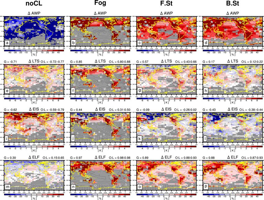
3042                                                     J. Shin and S. Park: The relationship between LCA and its proxies

subtropical and midlatitude marine stratocumulus decks. Al-       formed (CL0) if the inversion height is lower than zLCL . In
though uncertainty exists regarding whether the observed re-      general, the fractional area covered by stratiform clouds is
lationship between EIS and LCA is still maintained in the         larger than that of convective clouds. It is expected that a de-
future climate, EIS has been used to predict the variations in    tailed analysis of the relationship between LCA and various
LCA in response to climate changes (Caldwell et al., 2013;        proxies by individual CLs will provide insights regarding the
Qu et al., 2014, 2015). More recently, Kawai et al. (2017)        sources of the strengths and weaknesses of various proxies,
proposed an estimated cloud-top entrainment index (ECTEI)         which may help to develop a better proxy for LCA.
as a proxy for MSC, which is a modified EIS that takes into          The structure of this paper is as follows. Section 2 briefly
account cloud-top entrainment criteria.                           explains the conceptual framework of ELF including the data
   Although the aforementioned proxies (i.e., LTS, EIS, and       and analysis methods. Section 3 shows the results of the anal-
ECTEI) have been shown to be extremely useful in di-              ysis of the climatology and seasonal cycle of various CLs and
agnosing the variations in MSC over the subtropical and           the relationship between the amount when present (AWP),
midlatitude oceans, their applicability in the other regions      frequency (FQ), and amount (AMT) of individual CL and
(e.g., land, tropics, and high-latitude regions) has been in      various proxies. Several ways to develop an advanced ELF
question (in this regard, it may be more reasonable to            in the future are also discussed. A summary and conclusion
interpret LTS and EIS as cloud-controlling factors rather         are provided in Sect. 4.
than proxies for LCA). Park and Shin (2019) (PS19 here-
after) found that these proxies are not strongly correlated
with the observed LCA when the analysis domain is ex-             2     Method
tended over the entire globe and suggested an estimated
                                                                  2.1     Conceptual framework
low-level cloud fraction (ELF) as a new proxy for the anal-
ysis of the spatiotemporal variations in the global LCA.          PS19 provided a detailed description of the definition and
                                    √
ELF is defined as ELF = f · (1 − zLCL · zinv /1zs ), where        physical meaning of various proxies for LCA, which are
f = max[0.15, min(1, qv,ML /0.003)] is a freeze-dry factor        briefly summarized here. The lower tropospheric stability
with the water vapor specific humidity in the surfaced-based      (LTS) and estimated inversion strength (EIS) are defined as
mixed layer, qv,ML (kg kg−1 ); zLCL is the lifting condensation
level (LCL) of near-surface air; zinv is the inversion height     LTS ≡ θ700 − θsfc ,                                          (1)
estimated from the decoupling hypothesis suggested by Park                     m
                                                                  EIS = LTS + 0LCL           m
                                                                                   · zLCL − 0700 · z700 ,                      (2)
et al. (2004); and 1zs = 2750 m is a constant scale height.
PS19 showed that ELF is superior to LTS, EIS, and ECTEI           where θ700 and θsfc are the potential temperatures at 700 hPa
in diagnosing the spatial and temporal variations in the sea-                                          m and 0 m are the moist
                                                                  and the surface, respectively, and 0LCL         700
sonal LCA over both the ocean and land, including the ma-         adiabatic lapse rates of θ (units: K m−1 ) at the lifting conden-
rine stratocumulus deck, and explains approximately 60 %          sation level of near-surface air (zLCL ) and the 700 hPa height
of the spatial–seasonal–interannual variance of the seasonal      (z700 ), respectively. The estimated cloud-top entrainment in-
LCA over the globe, which is a much larger percentage than        dex (ECTEI; Kawai et al., 2017) is defined as
those explained by LTS (2 %) and EIS (4 %). PS19 also noted
several weaknesses of ELF, such as its tendency to underes-       ECTEI = EIS − β(Lv /cp )(qv,sfc − qv,700 ),                  (3)
timate LCA over deserts and the North Pacific and Atlantic
                                                                  where β = 0.23, Lv is the latent heat of vaporization, cp is
oceans and overestimate LCA in other regions.
                                                                  the specific heat at constant pressure, and qv,700 is the water
   In this study, we extend PS19 and examine the relationship
                                                                  vapor specific humidity at 700 hPa.
between LCA and its proxies by individual low-level cloud
                                                                     The estimated low-level cloud fraction (ELF) is defined as
type. Individual low-level cloud has its own distinct structure
of the planetary boundary layer (PBL) and synoptic environ-
                                                                                   √
                                                                                      zinv · zLCL
mental conditions (Norris, 1998; Norris and Klein, 2000). As      ELF ≡ f · 1 −                      = f · [1 − β2 ] ,        (4)
                                                                                        1zs
the PBL transitions from the well-mixed to a decoupled state,
                                                                                 √
surface-observed low-level clouds change from stratocumu-         where β2 = zinv · zLCL /1zs is a low-level cloud suppres-
lus (CL5, for which CL is a low-level cloud code used by sur-     sion parameter with a constant scale height 1zs = 2750 m,
face observers defined from WMO, 1975a; see also Park and         zinv is the inversion height,
Leovy, 2004) to cumulus under stratocumulus (CL8), stra-                                                  m
                                                                                                          0LCL
                                                                   zinv = −(LTS/0700 m )+z
tocumulus formed by the spreading out of cumulus (CL4),                                       700 + 1zs · 0 m
                                                                                                    m  700       m
and eventually to shallow (CL1), moderate (CL2), and pre-                = −(EIS/0 m ) + z
                                                                                                    0
                                                                                                  · LCL   + 1z · LCL
                                                                                                                     0
                                                                                                                         ,    (5)
                                                                                     700     LCL      m
                                                                                                   0700        s   0700m
cipitating deep cumulus (CL3) with an anvil (CL9). In the             zLCL ≤ zinv ≤ zLCL + 1zs ,
stable PBL, sky-obscuring fog (CL11) or fair weather stra-
tus (CL6) is likely to be observed when the inversion height      and f is the freeze-dry factor (Vavrus and Waliser, 2008)
is slightly higher than zLCL , but low-level cloud cannot be      defined as a function of water vapor specific humidity at the

Atmos. Chem. Phys., 20, 3041–3060, 2020                                              www.atmos-chem-phys.net/20/3041/2020/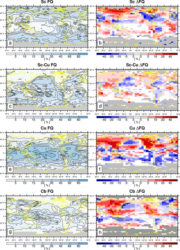
J. Shin and S. Park: The relationship between LCA and its proxies                                                              3043

surface (qv,sfc , unit: kg kg−1 ),                                   1975b. Table 1). In addition to the 10 CLs defined by the
          h               q        i                               WMO, EECRA defines two more CLs (CL10, sky-obscuring
                              v,sfc
f = max 0.15, min 1,                   .                      (6)    thunderstorm and shower, and CL11, sky-obscuring fog) by
                             0.003
                                                                     combining the present weather code with the observation
   Using the decoupling hypothesis of PLR04, PS19 esti-              of missing CL. Consequently, an individual EECRA obser-
mated zinv by assuming that the decoupling parameter α can           vation contains 12 CLs (from CL0 to CL11) and associ-
be parameterized as a linear function of the decoupled layer         ated LCA (from 0 to 8 octas) such that a set of 12 CLs
thickness, 1zDL ≡ zinv − zLCL ,                                      forms a complete basis function for the entire EECRA data.
      −
     θinv − θsfc

                     1zDL
                                                                    Based on similarities in morphology and physical property,
α≡ +             ≈          , 0 ≤ α ≤ 1,                 (7)         we grouped individual CLs into eight groups: noCL (no low-
     θinv − θsfc     1zs
                                                                     level cloud), fog (sky-obscuring fog), F.St (fair weather stra-
where θinv+              m ·(z                  −            m       tus), B.St (bad weather stratus), Sc (stratocumulus), Sc–Cu
             = θ700 −0700      700 −zinv ) and θinv = θsfc +0LCL ·
(zinv − zLCL ) are the potential temperatures just above and         (stratocumulus and cumulus), Cu (cumulus), and Cb (cumu-
below the inversion height (see Fig. 1 of PS19). In deriv-           lonimbus), in approximately the increasing order of vertical
ing ELF, it was assumed that the top of the surface-based            instability (see Table 2). Since ELF is based on the decou-
mixed layer is identical to zLCL . The freeze-dry factor is de-      pling hypothesis that can be applied in various regimes from
signed to reduce the parameterized cloud fraction in the ex-         the well-mixed to fully decoupled states, we included all CLs
tremely cold and dry atmospheric conditions typical of po-           in our analysis. For individual CLs or combinations of CLs,
lar and high-latitude winters.                                       we computed cloud frequency (FQ), amount when present
                              √ ELF can be also written as           (AWP), and amount (AMT), following the procedures de-
ELF = f ·[1−(zLCL /1zs ) 1 + (zinv − zLCL )/zLCL ], where
f is an increasing function of the amount of water vapor in          scribed in Hahn and Warren (1999) and Park and Leovy
the surface air, zLCL represents the degree of subsaturation of      (2004). Cloud FQ for a specific CL is defined by the fraction
near-surface air, and (zinv −zLCL )/zLCL quantifies the degree       of observations reporting the specific CL among the total set
of thermodynamic decoupling of the inversion base air from           of observations reporting any CL information. Cloud AWP
the surface air. ELF predicts that LCA increases as the near-        is the average LCA when a specific CL is observed. Cloud
surface air becomes more saturated with enough water vapor           AMT is the product of FQ and AWP.
and as the PBL becomes more vertically coupled, which is                Similar to PS19, individual EECRA cloud observations, as
consistent with what is expected to happen in nature. To en-         well as surface and upper-level meteorologies are averaged
sure 0 ≤ α ≤ 1 (i.e., thermodynamic scalars at the inversion         into 5◦ latitude × 10◦ longitude seasonal data for each year.
         −
base (θinv ) are bounded by the surface (θsfc ) and inversion top    To reduce the impact of random noise, a minimum of 10 ob-
   +
(θinv ) properties), the inversion height computed from Eq. (5)      servations were required to form effective seasonal grid data
was forced to satisfy zLCL ≤ zinv ≤ zLCL + 1zs .                     in each year. These seasonal grid data are used for computing
                                                                     annual climatologies and seasonal differences of various CLs
2.2   Data and analysis                                              (Figs. 1–2) and analyzing correlations between the LCA and
                                                                     various proxies by cloud type (Tables 1–2 and Figs. 3–6). In
The data used in our study are identical to those used in            addition, individual EECRA cloud observations are grouped
PS19. The surface observation data are from the Extended             into bins of individual proxies to better understand the con-
Edited Cloud Report Archive (EECRA; Hahn and Warren,                 tribution of individual CLs to the overall correlation relation-
1999), which compiles individual ship and land observations          ship between the proxies and LCA (Figs. 7–8). ECTEI pro-
of clouds, present weather, and other coincident surface me-         duced results very similar to those of EIS such that only the
teorologies every 3 or 6 h. The upper-level meteorologies            analysis for EIS is shown in this study.
(e.g., p and θ ) are from the ERA-Interim reanalysis prod-
ucts (ERAI; Simmons et al., 2007) at 6-hourly time intervals.
Spatial and temporal interpolations are performed to com-            3     Results
pute the upper-level meteorologies at the exact time and lo-
cation at which the EECRA surface observers reported the             3.1    Climatology and seasonal cycle
LCA. Our analysis uses the data from January 1979 to De-
cember 2008 (30 years) over the ocean and January 1979               Figures 1 and 2 show the annual climatology and the dif-
to December 1996 over land (18 years). Using the 6-hourly            ferences in the seasonal FQ of various CLs during JJA and
ERAI vertical profile of θ and water vapor interpolated to           DJF. As shown, noCL is frequently observed over the con-
individual EECRA surface observations, we computed LTS,              tinents but is rarely reported over the open ocean, implying
EIS, ECTEI, ELF, α, zLCL , and zinv .                                that one of the important factors controlling the formation of
   The surface observer reports cloud type (CL) and frac-            low-level clouds is the moisture source at the surface. One of
tional area (LCA) of low-level clouds following a strict hier-       the rare open-ocean areas with annual noCL FQ larger than
archy from the World Meteorological Organization (WMO,               10 % is the sea surface temperature (SST) cold tongue region

www.atmos-chem-phys.net/20/3041/2020/                                                 Atmos. Chem. Phys., 20, 3041–3060, 2020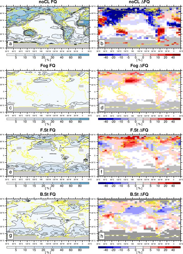
3044                                                          J. Shin and S. Park: The relationship between LCA and its proxies

Table 1. Low-level cloud (CL) specified by the WMO (CL0-CL9). EECRA defined two additional CLs – CL10 and CL11. When multiple
CLs exist, the observer is allowed to report only one CL as a representative CL following the coding priority. Among four cloud types (CL1,
CL5, CL6, and CL7), the cloud type that has the largest sky fraction has the highest priority. “Bad weather” denotes the conditions that
generally exist during precipitation and a short time before and after.

   CL      Nontechnical description                                                         Coding     Short name
   code                                                                                     priority
   0       No stratocumulus, stratus, cumulus, or cumulonimbus                              10         No low cloud
   1       Cumulus with little vertical extent and seemingly flattened                      By cover   Shallow cumulus
           or ragged cumulus other than of bad weather (or both)
   2       Cumulus of moderate or strong vertical extent,                                   5          Moderate cumulus
           generally with protuberances in the form of domes or towers,
           either accompanied (or not) by other cumulus or by stratocumulus
   3       Cumulonimbus, the summits of which at least partially lack sharp outlines        2          Cumulonimbus
           but are neither clearly fibrous (cirriform) nor in the form of an anvil;
           cumulus, stratocumulus, or stratus may also be present
   4       Stratocumulus formed by the spreading out of cumulus;                            3          Stratocumulus from cumulus
           cumulus may also be present
   5       Stratocumulus not resulting from the spreading out of cumulus                    By cover   Stratocumulus
   6       Stratus in a more or less continuous sheet or layer,                             By cover   Fair weather stratus
           in ragged shreds, or both, but no stratus fractus of bad weather
   7       Stratus fractus of bad weather, cumulus fractus of bad weather,                  by cover   Bad weather fractus
           or both (pannus), usually below altostratus or nimbostratus
   8       Cumulus and stratocumulus                                                        4          Cumulus under stratocumulus
           other than that formed from the spreading out of cumulus;
           the base of the cumulus is at a different level from that of the stratocumulus
   9       Cumulonimbus, the upper part of which is clearly fibrous (cirriform)             1          Cumulonimbus with anvil
           often in the form of an anvil, either accompanied (or not)
           by cumulonimbus without an anvil or fibrous upper part,
           by cumulus, stratocumulus, stratus, or pannus
   10      Sky is obscured (CL: missing with total cloud fraction N = 9)                    –          Sky-obscuring TS
           by thunderstorm shower (ww = 80–99)                                                         (thunderstorm shower)
   11      Sky is obscured (CL: missing with total cloud fraction N = 9)                    –          Sky-obscuring fog
           by fog (ww = 10–12, 40–49)

                                                                          in the eastern equatorial Pacific Ocean, where SST is lower
                                                                          than the overlying air temperature, net upward buoyancy flux
Table 2. Author-defined short names of low-level cloud (CL) types
used in our study.
                                                                          from the sea surface is very weak, and the atmospheric PBL
                                                                          is stable (Deser and Wallace, 1990). As a result, turbulent
  Abbreviation     CL code          Description
                                                                          vertical moisture transport from the sea surface to zLCL is
                                                                          strongly suppressed (i.e., zinv < zLCL ), resulting in the max-
  noCL             CL0              No low-level cloud                    imum FQ of noCL (Park and Leovy, 2004). This indicates
  Fog              CL11             Sky-obscuring fog                     that not only the moisture source at the surface, but also ver-
  F.St             CL6              Fair weather stratus                  tical stability in the atmospheric PBL controls the formation
  B.St             CL7              Bad weather stratus
                                                                          of low-level clouds. Over the continents and the Arctic area,
  Sc               CL5              Stratocumulus
  Sc–Cu            CL8 and CL4      Stratocumulus and cumulus
                                                                          noCL is more frequently observed during boreal winters than
  Cu               CL1 and CL2      Cumulus                               summers, presumably because strong daytime insolation dur-
  Cb               CL3 and CL9      Cumulonimbus                          ing summer destabilizes the lower troposphere, promoting
                                                                          the onset of convective clouds (i.e., Sc–Cu, Cu, and Cb).
                                                                          Strong nocturnal LW radiative cooling during winter stabi-

Atmos. Chem. Phys., 20, 3041–3060, 2020                                                     www.atmos-chem-phys.net/20/3041/2020/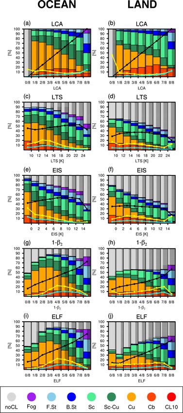
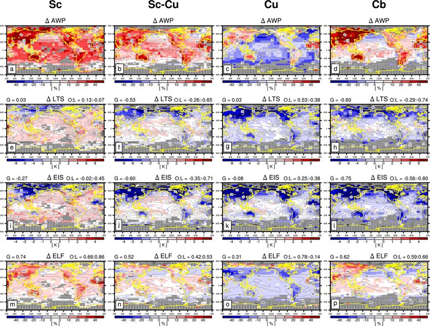
J. Shin and S. Park: The relationship between LCA and its proxies                                                           3045

lizes the lower troposphere, which forces zinv < zLCL . In ad-    3.2   Proxy vs. the AWP of individual low-level clouds
dition, the amount of moisture at the near surface is very
small during winter. Similar to the case over the SST cold        Figures 3 and 4 show the composite anomalies of LCA
tongue, strong vertical stability over the winter continents      and various proxies with respect to the seasonal climatol-
and Arctic area appears to increase the probability of the oc-    ogy when a specific CL was reported (see Figs. S1 and S2
currence of noCL, which appears to be somewhat opposite to        in the Supplement for the composite anomalies of zLCL , zinv ,
the embedded decoupling processes into ELF that increases         α, and 1 − β2 ). The anomalous LCA in the top row (1AWP)
as zinv decreases. However, with the freeze-dry factor, ELF       is the difference between the amount when present (AWP)
may be able to capture enhanced noCL frequency over the           when a specific CL was reported and climatological LCA.
continents during winter due to a small amount of moisture        To examine the coherency between 1AWP and the anoma-
near the surface. PS19 showed that the freeze-dry factor sub-     lies of individual proxies in each grid box, we computed the
stantially reduces ELF in this region during winter.              non-centered geographical correlation coefficients between
   Fog is frequently observed over the western North Pacific      1AWP and 1proxy over the entire globe (G), ocean (O),
and Atlantic oceans, including the Arctic area, during JJA        and land (L), respectively, which are shown at the top of the
when the Arctic sea ice melts and moist warm air is advected      individual plots. Here, we used the non-centered correlations
into the cold SST region across the midlatitude SST front.        rather than centered correlations to assess whether the spatial
This indicates the saturation of advected air parcels by the      means of 1AWP and 1proxy, as well as the spatial variabil-
contact cooling with the underlying cold SST or more up-          ities of those, are similar.
ward moisture transport from the open ocean over the Arctic,         When noCL is reported, AWP is zero, that is, 1AWP =
which can be captured by ELF through the decrease in zLCL .       −LCA in Fig. 3a. However, both LTS and EIS increase
F.St has a similar climatology and seasonal cycles as fog, im-    (G = −0.714 and −0.62 for LTS and EIS, respectively), par-
plying that the physical processes controlling the formation      ticularly over the far northern continents and Arctic area.
of fog are similar to those of F.St. B.St has an annual clima-    This is because noCL can occur when inversion is strong
tology similar to that of F.St, but its seasonal cycle over the   near the surface under dry conditions (Norris, 1998; Koshiro
North Pacific and Atlantic oceans is opposite to that of F.St,    and Shiotani, 2014). Conversely, ELF decreases in a desir-
with more frequency during boreal winters. Similar to B.St,       able way due to the freeze-dry factor (compare Fig. 3m with
Cb is more frequently observed during winter in this region,      Fig. S1m). Over the eastern subtropical marine stratocumu-
which is presumably due to the frequent passage of midlati-       lus deck, LTS, EIS, and ELF show a hint of negative anomaly
tude synoptic storms in winter. A composite analysis showed       which, however, is too weak to explain the substantial de-
that Cb is frequently observed on the rear side of the midlat-    crease in LCA when noCL is reported. Over the midlati-
itude synoptic cold front with a reduced lower tropospheric       tude oceans, the situation is worse and none of the factors
stability, while B.St is observed on the front or near center     comprising ELF (i.e., zLCL , zinv , and α) can explain the de-
of the synoptic storm with an enhanced lower tropospheric         crease in LCA (Fig. S1a, e, i). Although slightly better than
stability (Houze, 2014; Park and Shin, 2020). When the mid-       LTS and EIS, ELF has an apparent problem in diagnosing
latitude storm track passes, anomalous mean vertical motion       the decrease in LCA when noCL was reported, particularly
in the mid-troposphere drives the changes in the mid-level        over the ocean (O = 0.15). This problem worsens without the
clouds, but the variations in the lower tropospheric stability    freeze-dry factor (Fig. S1m). When fog, F.St, or B.St are re-
also drive the changes in LCA, which can be captured by           ported, LCA increases over the entire globe, which is very
ELF through the variations in zinv .                              well captured by ELF (G = 0.97, 0.89, and 0.88 for fog, F.St,
   In the Northern Hemisphere, Sc is frequently observed          and B.St, respectively), due to the simultaneous decreases in
over the eastern subtropical and midlatitude oceans during        zLCL , zinv , and α. Although slightly worse than ELF, LTS and
JJA, when the subtropical and midlatitude high is strong and      EIS also capture the increase in LCA when fog was reported
the PBL is relatively well coupled. In the Namibian and Peru-     (G = 0.85 and 0.44 for LTS and EIS, respectively). However,
vian stratocumulus decks west of South America and south-         undesirable negative anomalies of LTS and EIS over the far
ern Africa, Sc is most frequently reported during SON when        northern continents, including the Arctic area, worsen from
SST is at a minimum (Klein and Hartmann, 1993). Over most         fog to F.St and B.St, resulting in very weak (G = 0.17 for
ocean areas, seasonal variations in Sc tend to be opposite to     LTS) or even negative (G = −0.43 for EIS) correlations be-
those of Cu and Cb. ELF is designed to capture these con-         tween 1LTS–1EIS and 1AWP when B.St was reported. We
versions between Sc and Cu in association with the PBL de-        speculate that in these dry regions, the formation of fog, F.St,
coupling. Over northern Asia and Canada, including a por-         and B.St needs upward moisture transports from the surface,
tion of the Arctic area, both convective and stratiform clouds    which is likely to be accompanied by the reduction of verti-
are more frequently observed during boreal summers than           cal stability in the lower troposphere (e.g., breakup of sea ice
winters, presumably due to the destabilization of the lower       over the Arctic). As a result, 1LTS and 1EIS are negatively
troposphere by strong insolation heating and more surface         correlated with 1AWP over the far northern continents and
moisture.                                                         Arctic area. Overall, ELF is better than LTS and EIS in diag-

www.atmos-chem-phys.net/20/3041/2020/                                              Atmos. Chem. Phys., 20, 3041–3060, 2020
3046                                                         J. Shin and S. Park: The relationship between LCA and its proxies

Figure 1. (a, c, e, g) The annual mean climatological CL frequency (FQ) and (b, d, f, h) the differences in climatological CL FQ between JJA
and DJF (1FQ = FQ(JJA) − FQ(DJF)) for (a, b) noCL, (c, d) fog, (e, f) F.St, and (g, h) B.St. In the first column, the grid boxes with a total
observation number less than 100 are shaded with gray. In the second column, statistically insignificant 1FQ values at the 99.9 % confidence
level from the two-sided Student’s t test assuming independent samples are denoted by white, and the grid boxes with the observation number
less than 100 during either JJA or DJF are shaded with gray.

Atmos. Chem. Phys., 20, 3041–3060, 2020                                                    www.atmos-chem-phys.net/20/3041/2020/
J. Shin and S. Park: The relationship between LCA and its proxies                                     3047

Figure 2. Same as Fig. 1 but for Sc, Sc–Cu, Cu, and Cb.

www.atmos-chem-phys.net/20/3041/2020/                               Atmos. Chem. Phys., 20, 3041–3060, 2020
3048                                                         J. Shin and S. Park: The relationship between LCA and its proxies

Figure 3. Composite anomalies of (a–d) AWP (amount when present), (e–h) LTS, (i–l) EIS, and (m–p) ELF with respect to the annual
climatology when (a, e, i, m) noCL, (b, f, j, n) fog, (c, g, k, o) F.St, and (d, h, l, p) B.St were reported. 1AWP is the difference between
the AWP of a specific CL and climatological LCA. The contour line is the annual climatology of LCA and individual proxies. At the top of
individual plots, non-centered correlation coefficients between 1AWP and 1proxy over the globe (G), ocean (O), and land (L) are shown.
In each plot, statistically insignificant anomalies at the 99.9 % confidence level from the two-sided Student’s t test assuming independent
samples are denoted by white, and grid boxes with the observation number of a specific CL less than 100 are shaded by gray. Grid boxes
with a total observation number less than 100 are marked with a dot.

nosing the variations of fog and stratus over both the ocean            1LCA over land for Sc–Cu (L = −0.65/ − 0.71 for LTS and
and land. It should be noted that LTS, EIS, and ECTEI are               EIS), Cu (L = −0.38/ − 0.38), and Cb (L = −0.74/ − 0.80).
mainly designed to be used over the ocean without sea ice,              The negative correlation for Sc can be explained by the same
and they are not intended to be used over land and sea ice.             physical processes applied to the cases of fog, F.St, and B.St
   In addition to the fog and stratus, ELF captures the vari-           as explained above (i.e., enhanced moisture transport from
ations in LCA in association with Sc (G = 0.74), Sc–Cu                  the surface and associated decrease in vertical static stabil-
(G = 0.52), Cu (G = 0.31), and Cb (G = 0.62) reasonably                 ity). In the very dry regions where background LCA is very
better than LTS and EIS. When Sc was reported and LCA                   small, the onset of Cu and Cb in unstable situations (e.g., de-
increases, both LTS and EIS increase over the subtropical               creases in LTS and EIS) will result in the increase in LCA.
and midlatitude oceans. However, over the Arctic, Asia, and             Although generally better than LTS and EIS, ELF also has
deserts areas, LTS and EIS show negative anomalies opposite             a problem in capturing the increase in LCA over Asia and
to the increased LCA, which worsens and extends to other                most desert areas when Cu was reported (L = −0.14). In
continents from Sc and Sc–Cu to Cu and Cb, resulting in                 summary, an advanced ELF in the future should be designed
substantial negative correlations between 1LTS–1EIS and                 to capture the decrease in maritime LCA associated with

Atmos. Chem. Phys., 20, 3041–3060, 2020                                                    www.atmos-chem-phys.net/20/3041/2020/
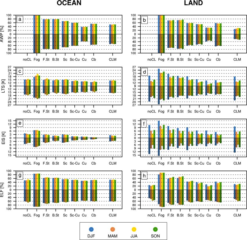
J. Shin and S. Park: The relationship between LCA and its proxies                                                          3049

Figure 4. Same as Fig. 3 but for Sc, Sc–Cu, Cu, and Cb.

noCL and the increase in continental LCA associated with          of the strongest deep convective system over the continents
Cu.                                                               in association with the gradual buildup of the mesoscale con-
   Figure 5 shows the area-averaged seasonal climatol-            vective organization forced by the evaporation of convective
ogy of the AWP and various proxies when a specific CL             precipitation (Park, 2014a, b). As a global proxy for the AWP
was reported over the ocean and land during the day-              of individual CLs, ELF shows more desirable inter-CL vari-
time (09:00–21:00) and nighttime (21:00–09:00), respec-           ations than LTS and EIS, which have strong ocean–land con-
tively (see Fig. S3 for zLCL , zinv , α, and 1 − β2 ). By defi-   trasts (in particular, EIS) and a seasonal cycle over land. The
nition, fog is always overcast, and stratiform clouds tend to     weaker seasonal cycle and ocean–land contrasts of ELF may
have larger AWP than convective clouds. Cb has larger AWP         imply opposite variations in zinv and zLCL . Due to the freeze-
than Cu, presumably due to larger cross-sectional and lat-        dry factor, ELF is slightly smaller than 1 − β2 during DJF
eral areas of deep convective updraft plumes or the contri-       over land, and the freeze-dry factor also contributes to re-
bution of detrained convective condensates. With the excep-       ducing the excessive seasonal cycle (compare Figs. 5h and
tion of Cb, AWP over the ocean is slightly larger than that       S3h). ELF has a somewhat stronger diurnal cycle than AWP
over land. The diurnal cycle of the AWP in most CLs is very       over land with a larger ELF during the night, which is pre-
weak. However, continental Cb during the night tends to have      sumably due in part to diagnosing the noCL condition as
a slightly larger AWP than during the day, which seems to be      a nonzero ELF, as will be explained later. The factors com-
contradictory to the intuition that deep cumulonimbus over        prising ELF (zLCL , zinv , and α) have fairly similar inter-CL
land is forced by strong insolation heating during the day.       variations, with larger values for convective than stratiform
This may reflect the late evening or nocturnal development        clouds (Fig. S3). Interestingly, zLCL for Cb is smaller than

www.atmos-chem-phys.net/20/3041/2020/                                              Atmos. Chem. Phys., 20, 3041–3060, 2020
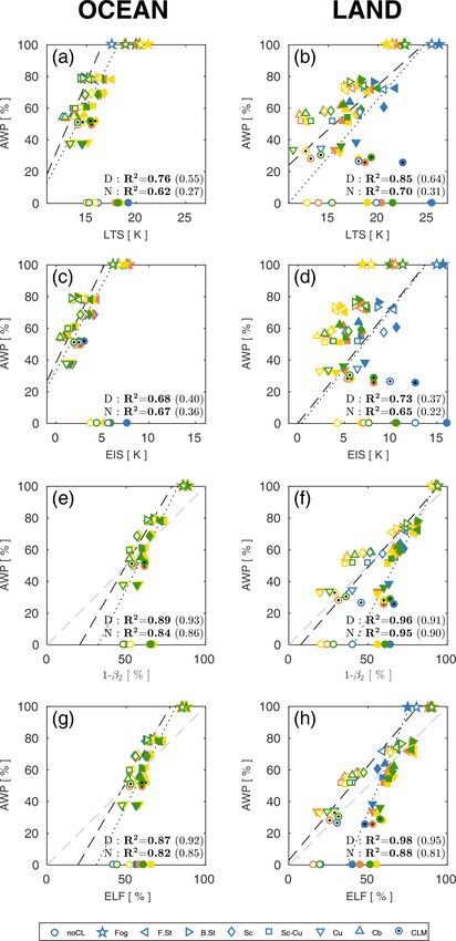
3050                                                          J. Shin and S. Park: The relationship between LCA and its proxies

Figure 5. Seasonal climatologies of the (a, b) AWP, (c, d) LTS, (e, f) EIS, and (g, h) ELF averaged over the (left) ocean and (right) land for
each season (DJF, MAM, JJA, and SON, denoted by different colors) during the daytime (09:00–21:00, upward bars with bright colors) and
nighttime (21:00–09:00, downward bars with dark colors) when a specific CL was reported. In each plot, CLM denotes the climatology for
all CLs.

that of Cu, presumably due in part to the evaporation of con-            types, ELF during the night tends to be larger than during the
vective precipitation and the associated moistening and latent           day, particularly over land, indicating that the product of zinv
cooling of near-surface air when Cb was reported.                        and zLCL during the day is larger than during the night. This
   Figure 6 shows the scatter plots of individual CL AWP as              is an anticipated result since shortwave radiative heating of
a function of LTS, EIS, 1-β2 , and ELF obtained from Fig. 5.             the surface during the day destabilizes the lower troposphere
If noCL is excluded, all proxies have very good correlations             (i.e., increases zinv ) and decreases the relative humidity of the
with the AWP of individual CLs, although ELF and 1 − β2                  near-surface air (i.e., increases zLCL ). Over land, however,
perform slightly better than LTS and EIS. If fog is also ex-             both ELF and 1 − β2 tend to have steeper regression slopes
cluded, the correlations between LTS–EIS and AWP are sub-                during the night than during the day. This is due in part to the
stantially degraded, whereas the performances of ELF and                 diagnosis of the noCL condition as a nonzero ELF, particu-
1 − β2 do not change much (see R 2 in parenthesis in Fig. 6).            larly during the night, when noCL conditions are frequently
Similar to the regression analysis of PS19, the slope of inter-          reported (see Fig. 1a). To be a better proxy for LCA (i.e.,
CL AWP regressed on ELF during the day over the ocean                    LCA = ELF denoted by the dashed gray line), ELF of noCL
is steeper than that over land. Over the ocean, the regression           (and Cu except over land during the day) should be much
slopes during the night are roughly similar to those during the          lower than the current values, while the ELFs of Sc, Sc–Cu,
day but with systematically higher proxy values. For all cloud           Cb, and Cu over land during the day as well as fog, F.St, and

Atmos. Chem. Phys., 20, 3041–3060, 2020                                                     www.atmos-chem-phys.net/20/3041/2020/
J. Shin and S. Park: The relationship between LCA and its proxies                                                                        3051

Figure 6. Scatter plots of Fig. 5 over the (a, c, e, g) ocean and (b, d, f, h) land during the daytime (open symbols) and nighttime (filled
symbols). Also plotted are the linear regression lines and squared correlation coefficients (R 2 ) during the daytime (D, dashed) and nighttime
(N, dotted). The bold R 2 values are when CLM and noCL are excluded in the regression analysis, and the R 2 values in parenthesis are when
fog is additionally excluded. The seasons are marked with the same colors as Fig. 5. The dashed gray lines in the last four plots denote
AWP = ELF.

www.atmos-chem-phys.net/20/3041/2020/                                                       Atmos. Chem. Phys., 20, 3041–3060, 2020
3052                                                      J. Shin and S. Park: The relationship between LCA and its proxies

B.St over the ocean should be higher than the current values.
These required behaviors are fairly consistent with the con-
clusion drawn from the analysis of Figs. 3 and 4. In contrast
to previous studies reporting a superior performance of EIS
compared to LTS, our analysis does not show a clear differ-
ence in their performances. This is presumably because our
study compared their performances over the entire globe in-
stead of marine stratocumulus decks, the main target areas of
EIS and LTS.

3.3    Proxy vs. the FQ of individual low-level clouds

Figure 7 shows stacked percentage plots of the frequencies
of individual CLs in the bins of various proxies, defined as
the number of observations reporting a specific CL divided
by the total observation number in each bin. Figure 7a, a plot
with a perfect proxy for LCA, shows that noCL exists en-
tirely in the 0 octa bin, fog only exists in the 8 octa bin, and
the bin AWP (black line) increases in a perfect linear way
as LCA increases, as expected. As LCA increases, the fre-
quency of Cu decreases but that of stratiform clouds (F.St,
B.St, Sc, and Sc–Cu) tends to increase. In contrast to Cu,
the frequency of Cb in the low octa bins gradually increases
with LCA. The observation number is relatively large in the
0 and 8 octa bins (yellow line). The low-level cloud AMT
contributed by individual bins (the cyan line that is a simple
product of the black and yellow lines) increases with LCA
but not in a perfectly linear way. The overall patterns over
land are approximately similar to those over the ocean. Over
land, the observation number is the largest in the 0 octa bin,
and convective clouds (Cu and Cb) are mostly observed dur-
ing the day. Any good proxy for LCA, if there is one, should
have similar patterns as Fig. 7a and b.
   The frequency of noCL increases as LTS and EIS increase,
which is mainly responsible for the undesirable decreases in
the AWP and AMT in the high bins of LTS and EIS. De-
signed as a proxy for marine stratocumulus, however, LTS
and EIS reasonably simulate the increase (decrease) in Sc
(Cu) frequency with LTS and EIS over the ocean. The in-
crease in noCL frequency with LTS and EIS seems to be
contradictory to our simple intuition that LTS and EIS are
positively correlated with LCA. However, we note that the
noCL condition is frequently reported with a strong inver-
sion near the surface when LTS and EIS are large (Norris,
1998; Koshiro and Shiotani, 2014). Note that the implied cor-      Figure 7. Stacked percentage plots for the FQs of individual CLs
                                                                   in the bins of various proxies: (a, b) LCA (i.e., a perfect proxy for
relation between LCA and EIS in Fig. 7e is weaker than in
                                                                   LCA), (c, d) LTS, (e, f) EIS, (g, h) 1-β2 , and (i, j) ELF over the (left)
previous studies (Wood and Bretherton, 2006), since LCA
                                                                   ocean and (right) land. AWP of all CLs in each bin is denoted by
in Fig. 7 is defined by including all low-level cloud types        the black line. The observation number FQ of individual bins (the
over the globe. In contrast to the case of LCA, fog exists in      ratio of the observation number in each bin to the total observation
several bins, and the frequency of Cb decreases monotoni-          number of entire bins) is denoted by the yellow line. LCA in each
cally with LTS and EIS. Similar to the case of LTS and EIS,        bin is denoted by the cyan line, which is the product of the black and
noCL exists ubiquitously in the entire ELF bins, indicating        yellow lines. The sum of the yellow line integrated over the entire
that the observed noCL conditions are frequently misinter-         bins is 100 %. The sum of the cyan line integrated over the entire
preted as cloudy conditions with LTS, EIS, and ELF. How-           bins is the global annual mean LCA. The bright and dark colors
ever, the frequency of noCL tends to decrease with ELF such        in each bar denote the fractions during the daytime and nighttime,
                                                                   respectively.

Atmos. Chem. Phys., 20, 3041–3060, 2020                                                www.atmos-chem-phys.net/20/3041/2020/
J. Shin and S. Park: The relationship between LCA and its proxies 3053
that the bin AWP increases in a desirable way as ELF in- Table 3. Spatial–seasonal correlation coefficients between various
creases, although the slope is smaller than the case of LCA. proxies and the frequency (FQ) of individual CLs. In contrast to
The frequency of noCL in the nonzero ELF bins over land Figs. 3 and 4 where non-centered correlation coefficients were com-
is substantially higher than that over the ocean. The obser- puted, the values in this table are the conventional centered correla-
vation number FQs in the 0 and 8 octa ELF bins are sub- tion coefficients computed from the climatological seasonal proxies
obtained by using all observations in each seasonal grid box instead
stantially lower than those in the LCA bins but higher in the
of the observations reporting a specific CL. In this table, LCA is
intermediate bins, implying that an advanced ELF needs to a perfect proxy for LCA. Statistically significant correlations at the
transfer the observation number FQ in the intermediate ELF 99.9 % confidence level from the Student’s t test assuming indepen-
bins into the 0 octa bin (e.g., by correctly diagnosing a noCL dent samples are denoted by bold.
condition) and 8 octa bin (e.g., by correctly diagnosing a fog
condition). CL Domain LTS EIS 1 − β2 ELF LCA
Table 3 shows spatial–seasonal correlation coefficients be-
noCL O 0.69 0.79 0.42 −0.46 −0.62
tween the frequency of individual CLs and various prox- L 0.28 0.47 −0.33 −0.69 −0.87
ies. In contrast to Figs. 3 and 4, Table 3 (also Table 4) G 0.46 0.64 −0.19 −0.67 −0.82
shows a conventional centered correlation between the sea-
Fog O 0.45 0.23 0.55 0.63 0.49
sonal climatologies (i.e., averaged over all observations) of
L 0.22 0.15 0.41 0.41 0.37
various proxies and individual CL frequency. LCA increases G 0.20 0.07 0.47 0.55 0.53
as the frequencies of sky-obscuring fog (fog), stratus (F.St,
F.St O 0.32 0.52 0.75 0.70 0.56
B.St), stratocumulus (Sc, Sc–Cu), and continental convec-
L 0.27 0.14 0.46 0.47 0.45
tive clouds (Cu, Cb) increase, and it decreases as the fre- G 0.22 0.27 0.61 0.60 0.54
quencies of noCL and marine convective clouds increase. Ex-
cept for marine Sc–Cu and continental Cu, ELF reproduces B.St O −0.15 0.15 0.36 0.47 0.70
L 0.01 −0.00 0.43 0.52 0.56
these correlation characteristics of LCA with individual CLs
G −0.16 −0.06 0.38 0.52 0.69
well, at least qualitatively. The freeze-dry factor substantially
contributes to the improved correlations of noCL with ELF Sc O 0.40 0.59 0.66 0.39 0.31
L 0.17 0.15 0.57 0.54 0.68
from β2 . As explained in PS19, the freeze-dry factor (f =
G 0.30 0.40 0.56 0.36 0.31
max[0.15, min(1, qv,sfc /0.003) ]) is designed to reduce a di-
agnosed LCA in a very dry region such that it is most effec- Sc–Cu O 0.01 −0.12 −0.08 0.03 0.28
tive over the far northern continents and Arctic area, particu- L −0.29 −0.50 −0.07 0.18 0.33
G −0.22 −0.43 0.05 0.27 0.50
larly during winter. Over the globe, noCL is negatively cor-
related with zinv and α (not shown), presumably due in part Cu O −0.36 −0.79 −0.78 −0.67 −0.53
to the frequent occurrence of noCL on the west coast of the L −0.49 −0.68 −0.30 0.01 0.19
G −0.45 −0.75 −0.30 −0.03 0.10
major continents and the equatorial SST cold tongue regions
where zinv is low due to cold SST (see Fig. 1a). The frequent Cb O −0.46 −0.38 −0.20 −0.21 −0.08
occurrence of noCL on the west coast is due to the advec- L −0.17 −0.17 0.14 0.21 0.35
tion of dry air from nearby continents (Mansbach and Norris, G −0.32 −0.31 0.03 0.08 0.17
2007). The frequent occurrence of noCL over the SST cold CLM O – – – – –
tongue is due to warm air advection from the south, the asso- L – – – – –
ciated stabilization of the lower PBL, and the suppression of G – – – – –
vertical moisture transport from the sea surface to zLCL (Park
and Leovy, 2004). Designed as proxies for marine stratocu-
mulus, LTS and EIS show a strong correlation with Sc FQ 3.4 Proxy vs. the AMT of individual low-level clouds
over the ocean. However, the correlation characteristics of
LTS and EIS with other CLs are less desirable than that of Figure 8 shows stacked plots of the AMT of individual CLs
ELF. For example, the correlations of LTS and EIS with fog, in the bins of various proxies. The LCA is the AMT of all
F.St, and B.St over the globe and continental Sc are signifi- CLs. The bin cloud AMT (the cyan line) increases monoton-
cantly weaker than those of LCA, and the correlation signs ically with LCA, with the largest increase from the 7 to 8
with noCL, Sc–Cu, and continental Cu and Cb are opposite octa bin (Fig. 8a, b). In the low bins, convective clouds con-
to those of ELF and LCA. One of the most unexpected as- tribute to the cloud AMT more than stratiform clouds, but in
pects of LTS and EIS is a strong positive correlation with the high bins, stratiform clouds contribute more. Total cloud
noCL FQ, as shown in Fig. 7. This may indicate a nonlinear AMT (i.e., the integration of the cyan line across the entire
response of clouds to the inversion strength or the existence bins) over the ocean is larger than that over land. In the 8
of other factors controlling the onset of noCL condition. octa bin over land, Cb contributes more than 20 % to the
cloud AMT. In contrast to LCA, none of the proxies show
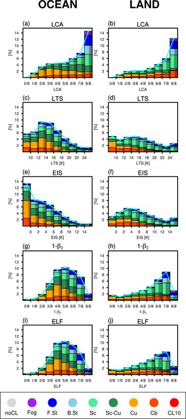
a required monotonic increase in the bin cloud AMT. Over
www.atmos-chem-phys.net/20/3041/2020/ Atmos. Chem. Phys., 20, 3041–3060, 20203054 J. Shin and S. Park: The relationship between LCA and its proxies
Table 4. Same as Table 3 but for the amount (AMT) of individual
CLs.
CL Domain LTS EIS 1 − β2 ELF LCA
noCL O – – – – –
L – – – – –
G – – – – –
Fog O 0.45 0.23 0.55 0.63 0.49
L 0.22 0.15 0.41 0.41 0.37
G 0.20 0.07 0.47 0.55 0.53
F.St O 0.32 0.51 0.76 0.72 0.60
L 0.29 0.18 0.48 0.49 0.48
G 0.22 0.27 0.62 0.62 0.58
B.St O −0.14 0.17 0.39 0.49 0.73
L 0.02 0.02 0.44 0.52 0.57
G −0.14 −0.03 0.40 0.53 0.71
Sc O 0.43 0.58 0.70 0.47 0.45
L 0.23 0.19 0.61 0.58 0.72
G 0.33 0.39 0.62 0.46 0.46
Sc–Cu O 0.09 −0.00 0.07 0.18 0.47
L −0.24 −0.46 0.00 0.24 0.41
G −0.17 −0.37 0.14 0.35 0.61
Cu O −0.34 −0.74 −0.70 −0.59 −0.36
L −0.44 −0.63 −0.21 0.07 0.28
G −0.43 −0.73 −0.23 0.03 0.22
Cb O −0.37 −0.16 −0.00 −0.06 0.08
L −0.08 −0.04 0.26 0.28 0.40
G −0.22 −0.13 0.17 0.15 0.23
CLM O −0.20 0.01 0.48 0.81 1.00
L −0.06 −0.21 0.58 0.82 1.00
G −0.23 −0.23 0.54 0.84 1.00
the ocean, EIS shows an undesirable monotonic decrease in
the bin cloud AMT, LTS is slightly better than EIS, and ELF
shows a further improvement, with the maximum bin cloud
AMT shifting to the higher bin. The improvement from EIS
and LTS to ELF is more pronounced over land, but the rapid
decrease in bin cloud AMT from the 7 to 8 octa ELF bins
is problematic. These variations in the bin cloud AMT are
largely controlled by the variations in the bin cloud FQ (see
the yellow line in Fig. 7). All proxies show the increase in
the relative contribution of stratiform clouds to the bin cloud
AMT as the bin value increases, but the contribution of Cb
AMT in the 8 octa bin over land is smaller than that of LCA.
Table 4 shows spatial–seasonal correlation coefficients be-
tween the AMT of individual CLs and various proxies. The
overall correlation characteristics of the cloud AMT are very
similar to those of the cloud FQ shown in Table 3. LCA tends Figure 8. Same as Fig. 7 but for the AMT of individual CLs in each
to increase as the cloud AMT of individual CLs increases. bin. The cyan lines are identical to those shown in Fig. 7. The sum
The only exception is marine Cu AMT that decreases as of all CL AMTs integrated over the entire bins is the global annual
LCA increases. ELF reproduces these correlation character- mean LCA, which is identical regardless of the proxies used for the
istics of the AMT of individual CLs with LCA well. As composite.
a global proxy for LCA, the correlation characteristics of
LTS and EIS with individual cloud AMT are less desirable
Atmos. Chem. Phys., 20, 3041–3060, 2020 www.atmos-chem-phys.net/20/3041/2020/J. Shin and S. Park: The relationship between LCA and its proxies 3055
than those of ELF: the correlations with continental Cu and a positive constant. This approach is likely to relocate the
Sc–Cu are unrealistically negative, and the correlations with observation frequency of noCL in the high ELF bins into the
sky-obscuring fog and stratus are much weaker than those of low ELF bins (Fig. 7i and j), reduce the large ELF values for
ELF and LCA. We note that LTS, EIS, and ECTEI are de- noCL (Fig. 6g and h), and improve the non-centered correla-
signed to be used over the ocean without sea ice, and they tions between 1ELF and 1LCA for various CLs including
are not intended to be used over land and sea ice. Table 4 noCL (Figs. 3 and 4).
indicates that a superior performance of ELF compared to Another apparent problem of the current ELF is the de-
LTS and EIS as a global proxy for LCA discovered by PS19 crease in ELF over desert areas (e.g., Sahara, Australia, and
(see the bottom row of Table 4) is derived from its realistic Saudi Arabia) when Cu was reported (see Fig. 4c and o).
correlations with various CLs rather than with a specific CL. In contrast to the ocean where the onset of Cu is often as-
sociated with the decoupling of the PBL and decreases in
3.5 What is necessary to further improve ELF as overlying marine stratocumulus and LCA (e.g., Bretherton,
a global proxy for LCA? 1992; Park et al., 2004), the onset of Cu over deserts with-
out the background stratocumulus seems to directly increase
We have shown that, generally, ELF diagnoses the inter-CL LCA. In this case, ELF tries to mimic the observed increase
variations in LCA better than LTS and EIS. However, we also in LCA by decreasing LCL (see Fig. S2c), but the larger in-
identified several weaknesses in ELF, such as the increase in creases in zinv and associated PBL decoupling seem to offset
ELF over the ocean when noCL was reported and the de- the impact of the reduced LCL, resulting in the decrease in
crease in ELF over deserts and Asian continents when Cu ELF. Conceptually, the current ELF is designed to mainly di-
was reported and LCA increases. In this section, we examine agnose the variations in stratiform clouds and detrained cu-
in more detail why ELF shows undesirable correlations with mulus at the inversion base, not the cumulus updraft plume
LCA for some cases and then provide a potential pathway to itself (see Fig. 1 of PS19), which is reflected in part by the
further improve ELF in the future. higher non-centered correlations between 1ELF and 1AWP
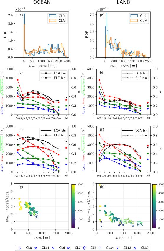
When noCL is reported, ELF increases over the North Pa- for stratiform clouds than for convective clouds as shown in
cific and North Atlantic oceans, which results in a very weak Figs. 3 and 4. To further improve the performance of ELF, it
non-centered correlation over the ocean (O = 0.15) between seems to be necessary to additionally diagnose the fraction
1LCA (Fig. 3a) and 1ELF (Fig. 3m). Although the correla- of cumulus updraft plume, particularly in regions without
tion over land (L = 0.65) is higher than over the ocean, the background stratiform clouds, such as deserts. Because the
magnitude of 1ELF is much smaller than 1LCA. As shown onset of Cu is closely associated with the PBL decoupling,
in Fig. 6g and h, noCL is the most distinct outlier from the de- one plausible approach is to incorporate a process to increase
sirable AWP = ELF line (dashed lines) in the inter-CL scatter ELF as δ∗ increases such that it can offset the decreases in
plots. This misdiagnosis of the noCL condition with nonzero stratocumulus and ELF with increasing δ∗ . If the aforemen-
p
ELF is also shown in Fig. 7i and j, and it worsens over land tioned ELF = f · [ 1 − (zLCL /1zs ) 1 + a · δ∗2 ] is adopted as
during the night. To understand this problem, we plotted the an advanced ELF, the contribution of the cumulus updraft
probability density function (PDF) of zDL ≡ zinv − zLCL us- plume can be incorporated by setting a to be smaller (or even
ing individual observations reporting noCL and compared it negative) than the default case, excluding the contribution of
with the PDF of entire observations (CLM) over the ocean the cumulus updraft plume. Potentially, a could be parame-
(Fig. 9a) and land (Fig. 9b). As shown, the PDF of near-zero terized as a decreasing function of zLCL .
zDL when noCL was reported is higher than that of CLM, √
Figure 9c–f show the variations in zLCL , zinv , zLCL · zinv ,
and the difference over land is larger than that over the ocean. and α as a function of ELF and LCA when Sc and Cu were
Conceptually, if zDL < 0 and so zinv < zLCL , low-level cloud reported over the ocean and land, respectively. When av-
cannot be formed such that LCA is likely to be small. This eraged over the entire bins (the “all” bin in the right col-
can happen when dry air at the surface is capped by a strong umn in each plot), Cu has higher zLCL , zinv , and α than
inversion such that vertical moisture transport from the sur- Sc, which is consistent with our conceptual understanding.
face to zLCL is inhibited. However, since √ our ELF = f · (1 − The increase in Cu AWP from the 0 to 1 octa bin over land
√
zinv · zLCL /1zs ) = f · [1 − (zLCL /1zs ) 1 + zDL /zLCL ] is is accompanied by the rapid increase in α (black solid line
formulated as a function of zinv = max(zinv ∗ ,z
LCL ) instead in Fig. 9f), presumably reflecting the onset of the cumu-
∗ ∗
of zinv (where zinv is the inversion height directly obtained lus updraft plume as the PBL is decoupled, which, as men-
from Eq. (5) without any clipping such that zinv∗ can be lower
tioned before, is not correctly captured by the current ELF
∗
than zLCL ), this case of zinv < zLCL is diagnosed as a highly (black dotted line in Fig. 9f). For both Sc and Cu (and also
cloudy condition in the current ELF. It seems that an ad- other CLs; not shown), zLCL tends to decrease monotoni-
vanced ELF needs to be able to simulate the decrease in LCA cally with LCA and ELF; however, zLCL and zinv decrease
with the increase in the absolute value of zDL∗ ≡ z∗ − z
inv LCL , more rapidly with ELF than with LCA. As a result, the de-
p √
such as ELF = f · [1 − (zLCL /1zs ) 1 + a · δ∗2 ], where δ∗ ≡ creasing rate of zinv · zLCL with ELF is much larger than
∗ /z
zDL LCL is a generalized decoupling parameter and a is that with AWP (green lines in Fig. 9c–f). One simple way
www.atmos-chem-phys.net/20/3041/2020/ Atmos. Chem. Phys., 20, 3041–3060, 20203056 J. Shin and S. Park: The relationship between LCA and its proxies
Figure 9. (a, b) Probability density functions (PDFs) of zDL = zinv − zLCL when noCL was reported (blue) and any CL was reported (red);
√
(c–f) zLCL (blue), zinv (red), α (black), and zLCL · zinv (green) in each octa bin of LCA (solid lines) and ELF (dashed lines) when (c, d) Sc
was reported and (e, f) Cu was reported, with the values averaged over the entire bins denoted by “all” in the right column. (g, h) The
√
distribution of 1zs,i = ( zinv · zLCL )/(1 − AWP/f ) (shaded; in meters) as a function of zLCL and δ ≡ zDL /zLCL for individual data points
shown in Fig. 6g and h. The plots in the left and right columns are over the ocean and land, respectively.
Atmos. Chem. Phys., 20, 3041–3060, 2020 www.atmos-chem-phys.net/20/3041/2020/J. Shin and S. Park: The relationship between LCA and its proxies 3057
to remedy this problem is to parameterize the scale height Over the North Pacific and Atlantic oceans, B.St and Cb are
√
1zs in ELF = f · (1 − zinv · zLCL /1zs ) as a function of ap- more frequently observed during DJF in association with the
propriate environmental variables, such as zinv , zLCL , and frequent passage of synoptic storms and the formation of
qv,sfc . To check whether this is a possible approach, we com- B.St (Cb) on the front (rear) side of the warm (cold) front
puted an ideal scale height 1zs,i in an ad hoc manner such where lower tropospheric stability is higher (smaller) than
that it exactly reproduces the observed LCA. More specifi- the climatology, which can be captured by ELF through the
cally, for individual data points shown in Fig. 6g and h, we changes in zinv . Sc is frequently observed over the eastern
√
computed 1zs,i = ( zinv · zLCL )/(1 − AWP/f ) by inverting subtropical and midlatitude oceans during JJA, and inter-
Eq. (4) (here, we implicitly assumed that 1zs used in Eq. (4) seasonal variations in Cu and Cb over most ocean areas tend
for deriving ELF differs from 1zs = 2750 m used in Eq. (5) to be opposite to those of Sc. ELF is designed to capture these
for deriving zinv , which is a completely reasonable assump- conversions between stratocumulus and cumulus in associa-
tion because there is no physical reason for 1zs in both equa- tion with the PBL decoupling.
tions to be identical). Figure 9g and h show the distribution We then examined the relationship between the anomalies
of 1zs,i in the phase space of zLCL and δ ≡ zDL /zLCL over of various proxies and AWP with respect to the climatology
the ocean and land, respectively. As shown, 1zs,i has a large when a specific CL was reported in each grid box (Figs. 3 and
inter-CL spread (and also relatively smaller seasonal and di- 4). When noCL was reported, LTS and EIS do not capture the
urnal spreads) instead of being a constant 2750 m. There is decrease in LCA and ELF has a similar problem except over
a tendency for fog and stratus to have larger 1zs,i than noCL the northern continents during winter when the freeze-dry
and convective clouds, and to the first order, 1zs,i seems factor operates. When stratiform clouds are reported, ELF
to increase as δ increases and zLCL decreases. Various CLs, captures the increase in LCA very well due to the simulta-
each of which have their own distinct PBL structure and neous decreases in zLCL , zinv , and α. With the exception of
AWP, seem to be reasonably separated from each other in this over the far northern continent and Arctic area, LTS and EIS
phase diagram, implying a possibility to parameterize 1zs as also work well, but their performance for F.St and B.St is de-
a function of zLCL and δ. Because an advanced ELF needs graded, mainly due to undesirable anomalies over Asia and
to incorporate other aspects discussed in the above two para- the Arctic area. As well as fog and stratus, ELF captures the
graphs, which will presumably involve some changes in the variations in LCA reasonably well when stratocumulus and
functional form of ELF, we leave a detailed parameterization cumulus are reported and significantly better than LTS and
of 1zs for future research. EIS. However, when Cu was reported over Asia and most
desert areas, ELF, as well as LTS and EIS, had a problem in
capturing the increase in LCA. ELF shows more consistent
4 Summary and conclusion inter-CL variations with the AWP of individual CLs than LTS
and EIS, which have ocean–land contrasts and a seasonal cy-
We extended the previous work of Park and Shin (2019) cle over land that are too strong (Fig. 5). The scatter plots be-
to examine the relationship between various proxies (i.e., tween various proxies and individual CL AWP showed that
LTS, EIS, ECTEI, and ELF) and LCA of individual low-level if noCL is excluded, LTS, EIS, and ELF have very good cor-
cloud types (CLs). An individual CL has its own distinct PBL relations with the AWP of individual CLs, although ELF per-
structure such that a detailed analysis of the relationship be- forms slightly better than LTS and EIS (Fig. 6). To be a bet-
tween various proxies and LCAs of individual CLs can pro- ter proxy for LCA, the ELF for noCL and Cu over ocean and
vide insights into the strengths and weaknesses of individual nocturnal land should be reduced, while the ELF for fog and
proxies, which may help to develop a better proxy in the fu- Cu over land during the daytime should be enhanced.
ture. We also analyzed individual CL frequency in the bins of
Firstly, we compared the annual climatology and seasonal various proxies. In the case of the perfect proxy for LCA
cycle of individual CL frequency (Figs. 1 and 2). The noCL (i.e., LCA itself), the frequency of Cu (stratiform clouds) de-
condition is frequently reported over the winter continents creases (increases) with LCA; convective clouds are mostly
and Arctic area but is seldom reported over the open ocean observed during the day, particularly over land; noCL exists
except in the eastern equatorial SST cold tongue region entirely in the 0 octa bin; the bin AWP increases in a perfect
where the PBL is stable in association with negative surface linear way as LCA increases; and the observation number
buoyancy flux. By construction, ELF has a limitation in cor- FQ is the largest in the 0 (particularly over land) and 8 octa
rectly diagnosing reduced cloudiness with enhanced stability bins. Similar to the perfect proxy, LTS, EIS, and ELF simu-
in this region. Fog and F.St are frequently observed over the late the decrease in Cu FQ (increase in stratiform cloud FQ)
summer western North Pacific–Atlantic oceans and Arctic from the low to high bins reasonably. However, all proxies
area, presumably due in part to the cooling of northward- incorrectly diagnose the observed no low-level cloud con-
advected air parcels and enhanced upward moisture flux ditions (noCL) as cloudy conditions (more severely for LTS
through the ice-free Arctic Ocean during summer. These pro- and EIS), resulting in unrealistic distributions of the bin AWP
cesses can be captured by ELF through the decrease in zLCL . and observation number FQ across the bins. The analysis of
www.atmos-chem-phys.net/20/3041/2020/ Atmos. Chem. Phys., 20, 3041–3060, 2020You can also read