Light Scattering from Filaments
←
→
Page content transcription
If your browser does not render page correctly, please read the page content below
1

                           Light Scattering from Filaments
                                       Arno Zinke and Andreas Weber, Member IEEE
                   Institut für Informatik II, Universität Bonn, Römerstr. 164, 53117 Bonn, Germany

   Abstract— Photo realistic visualization of a huge number of         similar to Bidirectional Scattering-Surface Reflectance Dis-
individual filaments like in the case of hair, fur or knitwear, is     tribution Functions (BSSRDF) and Bidirectional Scattering
a challenging task: Explicit rendering approaches for simulating       Distribution Functions (named BSDF) for surfaces in order
radiance transfer at a filament get totally impracticable with
respect to rendering performance, and it is also not obvious           to describe the radiance transfer at a fiber. The basic idea is
how to derive efficient scattering functions for different levels      to locally approximate this radiance transfer by a scattering
of (geometric) abstraction or how to deal with very complex            function on the minimum enclosing cylinder of a straight
scattering mechanisms. We present a novel uniform formalism for        infinite fiber, which is a first order approximation with respect
light scattering from filaments in terms of radiance, which we call    to the curvature of the filament. We call this approximation a
Bidirectional Fiber Scattering Distribution Function (BFSDF).
We show that previous specialized approaches, which have been          Bidirectional Fiber Scattering Distribution Function (BFSDF),
developed in the context of hair rendering, can be seen as             which can be seen as a special BSSRDF that is not defined
instances of the BFSDF. Similar to the role of the BSSRDF for          on the surface, but on the fiber’s local minimum enclosing
surface scattering functions, the BFSDF can be seen as a general       cylinder. (See section IV).
approach for light scattering from filaments which is suitable            2) Systematic derivation of less complex scattering func-
for deriving approximations in a canonic and systematic way.
For the frequent cases of distant light sources and observers we       tions: Based on the BFSDF we then derive further less
deduce an efficient far field approximation (Bidirectional Curve       complex scattering functions for different levels of (geometric)
Scattering Distribution Function, BCSDF). We show that on the          abstraction and for special lighting conditions, cf. Fig. 1. With
basis of the BFSDF parameters for common rendering techniques          the help of such scattering functions efficient physically based
can be estimated in a non ad-hoc, but physically based way.            visualizations—adapted to a desired rendering technique or
  Index Terms— Three-Dimensional Graphics and Realism –                quality—are possible. Furthermore the BFSDF allows for sys-
Shading, Light Scattering, Hair Modeling, Cloth Modeling               tematic comparisons and classifications of fibers with respect
                                                                       to their scattering distributions, since it provides a uniform
                       I. I NTRODUCTION                                and shape independent radiance parameterization for filaments.
   Physically based visualization of filaments like hair, fur,         (See sections V, VI and VII.)
yarns, or grass can drastically improve the quality of a render-          3) General framework for existing models for hair render-
ing in terms of photo realism. As long as the light transport          ing: Moreover, we show that the existing models developed
mechanisms for light scattering are understood, rendering a            for hair rendering [1], [2] can be integrated in our framework,
single filament is usually not very challenging. In this case the      which also gives a basis to discuss their physical plausibility.
filament could be basically modeled by long and thin volumes           (See section VIII.)
having specific optical properties like index of refraction               4) Derivation of analytical solutions and approximations
or absorption coefficient. However, for the frequent case of           for special cases: We furthermore address some special cases
a scene consisting of a huge number of individual fibers               where analytical solutions or approximations are available, e.g.
(like hair, fur or knitwear) this explicit approach becomes            a general BCSDF for opaque fibers (mapped with a BRDF) is
impracticable with respect to rendering performance. It is also        derived. In this context we also derive a flexible and efficient
not clear a priori, how to deal with very complex or unknown           near field shading model for dielectric fibers that accurately
scattering mechanisms or how efficient visualizations of fibers        reproduces the scattering pattern for close ups but can be
based on measurement data could be implemented.                        computed much more efficiently than particle tracing (or an
   Although progress has been made in rendering particular             equivalent) that was typically used to capture the scattering
fibers with particular lighting settings no general formulation        pattern correctly. (See section IX.)
has been found. As a result some more or less accurate models             5) Integration into existing rendering systems: We are able
for specific fibers and illumination conditions were developed,        to propose approximations of the BFSDF, which translate it to
especially in the realm of hair rendering [1], [2], [3], [4], [5].     some position dependent BSDF and preserves subtle scattering
If the viewing or lighting conditions change such models may           details thus allowing an integration into existing rendering
fail or have to be adopted.                                            kernels that can cope with BSDF and polygons only. (See
                                                                       section X.)
Our Contribution                                                                            II. P REVIOUS W ORK
   1) Introduction of novel general concept for radiance trans-           Bidirectional Scattering Distribution Functions (BSDF) re-
fer at a fiber: In this paper we introduce a novel concept             late the incoming irradiance at an infinitesimal surface patch to
  Accepted for publication by IEEE Transactions on Visualization and   the outgoing radiance from this patch [6]. It is an abstract op-
Computer Graphics; c IEEE.                                             tical material property which implies a constant wave length, a
2

                                                                       Fig. 2. Left: Incoming and outgoing radiance at a filament. Right: An
                                                                       ”intuitive” variable set for parameterizing incoming and outgoing radiance at
                                                                       the minimum enclosing cylinder. In this example the local cross section shape
                                                                       of the filament is pentagonal. The vector ~u denotes the local tangent (axis), s
                                                                       the position along this axis. The angles α and β span a hemisphere over the
                                                                       the surface patch at s, with α being measured with respect to ~    u within the
                                                                       tangent plane and β with respect to the local surface normal ~  n. Note that D~
                                                                       represents both incoming and outgoing directions.

Fig. 1.   Overview of the BFSDF and its special cases. The effective   cross section of a single yarn with respect to the arrangement
dimensions of the scattering functions are indicated on the left.
                                                                       of individual yarn fibers and then translate it along a three
                                                                       dimensional curve to form the entire filament. The results
                                                                       are looking quite impressive, but the question how to deal
light transport taking zero time and being temporally invariant
                                                                       with yarns with more complex scattering properties is not
as well. Having the BSDF of a certain material, the local
                                                                       addressed. A similar idea was presented by [12]. Here all
surface geometry and the incoming radiance, the outgoing
                                                                       computations base on a structure called lumislice, a light
radiance can be reconstructed. This BSDF concept works well
                                                                       field for a yarn-cross-section. However, the authors do not
for a wide range of materials but has one major drawback:
                                                                       address the problem of computing a physically based light
Incoming irradiance contributes only to the outgoing radiance
                                                                       field according to the properties of a single fiber of the yarn.
from a patch, if it directly illuminates this patch. Therefore it
                                                                          Adabala et al. [13] describe another method for visualizing
has to be generalized to take into account light transport inside
                                                                       woven cloth. Due to the limitations of the underlying BRDF
the material. This generalization is called a Bidirectional Sur-
                                                                       (Cook-Torance microfacet BRDF) realistic renderings of yarns
face Scattering Distribution Function—BSSRDF [6]. Several
                                                                       with more complex scattering properties remain a problem.
papers have addressed some special cases mainly in the context
                                                                       In the realm of applied optics light scattering from straight
of subsurface scattering [7], [8].
                                                                       smooth dielectric fibers with constant and mainly circular
   Further scattering models like BTF or even more gener-
                                                                       or elliptical cross sections were analyzed in a number of
alized radiance transfer functions have been introduced to
                                                                       publications [14], [15], [16], [17], [18]. Schuh et al. [19]
account for self-shadowing and other mesoscopic and macro-
                                                                       introduced an approximation which is capable of predicting
scopic effects [9].
                                                                       scattering of electro magnetic waves from curved fibers, too.
   Marschner et al. [2] presented an approach specialized for          All these approaches are of very high quality, but are either
rendering hair fibers. They very briefly introduce a novel curve       more specialized in predicting the maxima positions of the
scattering function defined with respect to curve intensity            scattering distribution or rather impractical for rendering pur-
(intensity scattered per unit length of the curve) and curve           poses because of their high numerical complexity.
irradiance (incoming power per unit length). Unfortunately no
hint about how it can be derived for other types of fibers
                                                                                           III. BASICS AND N OTATIONS
than hair is given. One major restriction of the scattering
model is that both viewer and light sources have to be distant         A. Motivation and General Assumptions
to the hair fiber. Therefore it is not suitable for rendering             We want to apply the basics of the radiometric concepts for
complex illumination like for example indirect illumination            surfaces in the realm of fiber optics. The general problem is
and hair-hair scattering, which is especially important for light      very similar: How much radiance dLo scattered from a single
colored hair [3]. Close-ups remain a problem, too. To fix those        fiber one would observe from an infinitesimal surface patch
problems the scattering model was extended to a specialized            dAo in direction (αo , βo ), if a surface patch dAi is illuminated
near field approach [3].                                               by an irradiance Ei from direction (αi , βi ) (cf. Fig. 2, Left).
   Another application of fiber rendering is the visualization of         This interrelationship could be basically described by a
woven cloth, where optical properties of a single yarn have to         BSSRDF at the surface of the fiber. Such a BSSRDF would
be taken into account. A method for predicting a corresponding         in general depend on macroscopic deformations of the fiber,
BSDF based on a certain weaving pattern and on dielectric              how the fiber is oriented and warped. As a consequence local
fibers was developed by Volevich et al. [10]. Gröller et al.          (microscopic) fiber properties could not be separated from
proposed a volumetric approach for modeling knitwear [11].             its global macroscopic geometry. Furthermore, all radiometric
They first measure the statistical density distribution of the         quantities must be parameterized with respect to the actual
3
surface of the filament, which may be not well defined—as
e.g. in the case of a fluffy wool yarn.
Therefore we define a BSSRDF on the local infinite min-
imum enclosing cylinder rather than on the actual surface of
the fiber in order to make the parameterization independent of
the fiber’s geometry. Thus the radiance transfer at the fiber is
locally approximated by a scattering function on the minimum
enclosing cylinder of a straight infinite fiber, which means a
first order approximation with respect to the curvature. We
Fig. 3. Left: Parameterization with respect to the normal plane and filament
call this function a Bidirectional Fiber Scattering Distribution axis (tangent) ~ ~ 0 denotes the projection of a direction D
u. The vector D ~ onto
Function (BFSDF). This approximation is accurate, if the the normal plane. The angle θ ranges from −π/2 to π/2, with θ = π/2 if ~ u
influence of curvature to the scattering distribution can be and D~ are pointing in the same direction. Right: Azimuthal variables within
neglected. This is the case e.g. if the normal plane. The parameter h is an offset position at the perimeter. Note
that parallel rays have same ϕ (measured counterclockwise with respect to
• the filament’s curvature is small compared to the radius ~
u) but different h.
of its local minimum enclosing cylinder or
• most of the incoming radiance only locally contributes to
outgoing radiance. of a direction with respect to the normal plane, ϕ its azimuthal
The latter condition is satisfied for instance by opaque wires, angle with respect to a fixed axis ~v and h an offset position of
since only reflection occurs and therefore no internal light the surface patch at the minimum enclosing cylinder, measured
transport inside the filament takes place. Hence the scattering within the normal plane. The variable s is the same as
is a purely local phenomenon and the curvature of the fiber introduced before and always means the position along the
plays no role at all. The former condition for instance holds axis of the minimum enclosing cylinder (Fig. 3).
for hair and fur. In this case substantial internal light transport We will now derive some useful transformation formulae
takes place, but since the curvature is small compared to the for variables of both sets.
radius and since the light gets attenuated inside the fiber, The projection of the angle of incidence at the enclosing
the differences compared to a straight infinite fiber may be cylinder onto the normal plane γ 0 is given by the following
neglected. The higher the curvature and the more internal two equations:
light transport takes place, the bigger the potential error that
cos β
is introduced by the BFSDF. cos γ 0 = (1)
cos θ
0
γ = |arcsin h| (2)
B. Notations
Before technically defining the BFSDF we will give an Thus for the spherical angle β we have
overview of our notations, which follow [2] in general. √
The local filament axis is denoted ~u and we refer to the β = arccos cos θ 1 − h2 (3)
planes perpendicular to ~u as normal planes. All local surface
The following relation holds between ξ, ϕ and h, cf. Fig. 3:
normals lie within the local normal plane. All incoming and
outgoing radiance is parameterized with respect to the local
ϕ + arcsin h 0 ≤ ϕ + arcsin h < 2π
minimum enclosing cylinder with radius r oriented along ξ= 2π + ϕ + arcsin h ϕ + arcsin h < 0 (4)
~u and is therefore independent of the actual cross section
ϕ + arcsin h − 2π ϕ + arcsin h ≥ 2π
geometry of the filament (Fig. 3 Left).
We introduce two sets of variables, which are suitable for The spherical coordinate α equals the angle between the
certain measurement or lighting settings. The first parameter ~ onto the local tangent plane and ~v . Since the
projection of D
set describes every infinitesimal surface patch dA at the angle between D~ and ~v is given by π/2−θ and the inclination
enclosing cylinder by its tangential position s and its azimuthal ~ with respect to the tangent plane is π/2 − β one obtains:
of D
position ξ within the normal plane (cylindrical coordinates).
The directions of both incoming and outgoing radiance are cos α = cos (π/2 − θ) / cos (π/2 − β)
then given by two spherical angles α and β which span a = sin θ/ sin β (5)
hemisphere at dA oriented along the local surface normal of sin θ
the enclosing cylinder (Fig. 2 Right, Fig. 3 Right). = p
1 − (1 − h2 ) cos2 θ
Typically this very intuitive way to parameterize both
directions and positions is not very well suited to actual Furthermore, the actual angle depends on the sign of h:
problems. In particular, this is the case for data acquisition and
many “real world” lighting conditions. Hence, we introduce
a second set of variables according to [2]. This set can be arccos √
sin θ
, h ≤ 0,
1−(1−h2 ) cos2 θ
split into two groups, one parameterizing all azimuthal features α= (6)
within the normal plane (h, ϕ) and another parameterizing all 2π − arccos
√ sin θ
, h > 0.
1−(1−h2 ) cos2 θ
longitudinal features (s, θ). The angle θ denotes the inclination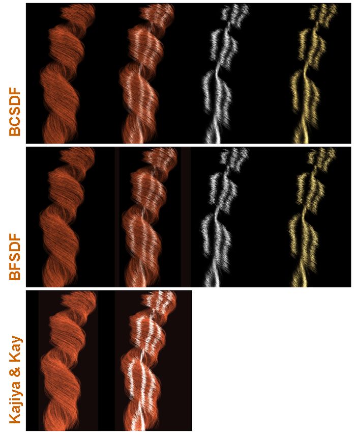
4

 IV. B IDIRECTIONAL F IBER S CATTERING D ISTRIBUTION
                F UNCTION — BFSDF

   We now technically define the Bidirectional Fiber Scattering
Distribution Function (BFSDF) of a fiber. The BFSDF relates
incident flux Φi at an infinitesimal surface patch dAi to the
outgoing radiance Lo at another position on the minimum
enclosing cylinder:
                                                                                     Fig. 4.    Left: Cross section of three very densely packed fibers. The
                fBFSDF (si , ξi , αi , βi , so , ξo , αo , βo ) :=                   problematic intersection of two enclosing cylinders is marked by an ellipse.

                    dLo (si , ξi , αi , βi , so , ξo , αo , βo )                     Fig. 5. Right: A slice at the minimum enclosing cylinder illuminated by
                                                                 .             (7)   parallel light and viewed by a distant observer.
                             dΦi (si , ξi , αi , βi )
Using the BFSDF the local orientation of a fiber and the in-
coming radiance Li , the total outgoing radiance of a particular                     Reparameterizing the scattering integral yields:
position can be calculated by integrating the irradiance over                        Lo (so , ho , ϕo , θo ) =
all surface patches and all incoming directions as follows:                                              π/2
                                                                                          +∞Z1 Z2π Z
                                                                                          Z
                                                                                                                 ∂ (ξi , αi , βi )
      Lo (so , ξo , αo , βo ) =
                                                                                                                 ∂ (hi , ϕi , θi )
           +∞Z2π Z2π Z
           Z             π/2                                                              −∞ −1 0 −π/2

                             fBFSDF (si , ξi , αi , βi , so , ξo , αo , βo )                  fBFSDF (∆s, hi , ϕi , θi , ho , ϕo , θo ) Li (si , hi , ϕi , θi )
                                                                                              q                        q
           −∞ 0      0   0                                                                      1 − cos2 θi (1 − h2i ) 1 − h2i cos θi dθi dϕi dhi d∆s.
               Li (si , ξi , αi , βi ) sin βi cos βi dβi dαi dξi dsi . (8)
                                                                                                                                                              (11)
For physically based BFSDF the energy is conserved, thus                             The above equation can be finally simplified to the following
all light entering the enclosing cylinder is either absorbed or                      equation:
scattered. In case of perfectly circular symmetric filaments the
BFSDF in addition satisfies the Helmholtz Reciprocity:                                   Lo (so , ho , ϕo , θo ) =
                                                                                              +∞Z1 Z2π Z
                                                                                              Z              π/2
              fBFSDF (si , ξi , αi , βi , so , ξo , αo , βo ) =
                                                                                                                  fBFSDF (∆s, hi , ϕi , θi , ho , ϕo , θo )
                  fBFSDF (so , ξo , αo , βo , si , ξi , αi , βi ) .            (9)
                                                                                               −∞ −1 0 −π/2

If the optical properties of a fiber are constant along s, then                                  cos2 θi Li (si , hi , ϕi , θi )     dθi dϕi dhi d∆s.         (12)
the BFSDF does not depend on si and so but on the difference
∆s := so − si . Thus the dimension of the BFSDF function                             This form of the scattering integral is especially suitable
decreases by one and the scattering integral reduces to the                          when having distant lights, i.e. parallel illumination, since
following equation:                                                                  parallel rays of light have same ϕi and θi but different
                                                                                     hi . Consider for example directional lighting, which can be
                                                                                     expressed by the radiance distribution L(ϕ0i , θi0 , ϕi , θi ) =
      Lo (so , ξo , αo , βo ) =                                                      E⊥ (ϕ0i , θi0 )δ(ϕi − ϕ0i )δ(θi − θi0 )/ cos θi with normal irradiance
           +∞Z2π Z2π Z   π/2
                                                                                     E⊥ (ϕ0i , θi0 ). Substituting the radiance in the scattering integral
                                                                                     by this distribution yields:
           Z
                             fBFSDF (∆s, ξi , αi , βi , ξo , αo , βo )
           −∞ 0      0   0                                                               Lo (ho , ϕo , θo ) = E⊥ (ϕ0i , θi0 ) cos θi0
                                                                                              +∞Z1
               Li (si , ξi , αi , βi ) sin βi cos βi dβi dαi dξi d∆s.(10)                     Z
                                                                                                       fBFSDF (∆s, hi , ϕ0i , θi0 , ho , ϕo , θo ) dhi d∆s.(13)
  This special case is an appropriate approximation for the                                   −∞ −1
general case if the following condition is satisfied:
                                                                                     All formulae derived in this section hold for a single filament
  •    The cross section shape and material properties vary                          only. But a typical scene consists of a huge number of
       slowly or at a very high frequency with respect to s.                         densely packed fiber assemblies. Since incoming and outgoing
Good examples for high frequency detail are cuticula tiles of                        radiance was parameterized with respect to the minimum en-
hair fibers or surface roughness due to the microstructure of                        closing cylinder, those cylinders must not intersect. Otherwise
a filament. Since the latter assumption is at least locally valid                    it can not be guaranteed that the results are still valid (Fig. 4).
for a wide range of different fibers we will restrict ourselves                      If a cross section shape closely matches the enclosing cylinder
to this case in the following.                                                       the maximum overlap is very small. Hence, computing the
   The BFSDF and its corresponding rendering integral was                            light transport at a projection of the overlapping regions onto
introduced with respect to the “intuitive variable set” first.                       the enclosing cylinder can be seen as a good approximation
We now derive a formulation for the second variable set.                             of the actual scattering.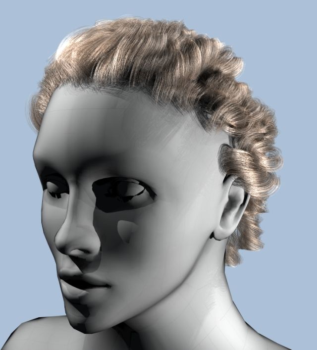
5

                      V. D IELECTRIC F IBERS                               Note that the factor (cos θi )−2 in front of the equation
                                                                        compensates for
   Since most filaments consist of dielectric material it is
very instructive to discuss the scattering at dielectric fibers.           • the integration measure with respect to θi ,hi and ϕi which

For perfectly smooth dielectric filaments with arbitrary but                  contributes a factor of (cos θi )−1 and
constant cross section the dimension of the BFSDF reduces                  • the cosine of the angle of incidence which gives another

from seven to six. This is a direct consequence of the fact that              (cos θi )−1 .
light entering at a certain inclination will always exit at the            Even though this kind of BFSDF is for smooth dielectric
same inclination (according to absolute value), regardless of           materials with absorption and locally constant cross section
the sequence of refractions and reflections it undergoes.               only, its basic structure is very instructive for a lot of other
   The incident light is reflected or refracted several times           types of fibers, too. For example internal volumetric scat-
before it leaves the fiber. The amount of light being reflected         tering or surface scattering—due to surface roughness—do
resp. refracted is given by Fresnel’s Law. At each surface              not change this basic structure in most cases but result in
interaction step the scattered intensity of a ray decreases—            spatial and angular blurring, cf. Fig. 7. By replacing the δ-
except in case of total reflection. If absorption inside the fiber      distributions in the BFSDF for smooth dielectric cylinders—
takes place, then loss of energy is even more prominent. Since          cf. eqn. (15)—with normalized lobes (like Gaussians) centered
an incoming ray of light does not exhibit spatial or angu-              over the peak similar effects can be simulated easily.
lar blurring, the BFSDF is characterized by discrete peaks.                The presence of sharp peaks in the scattering distribution is
Therefore, it makes sense to analyze only those scattering              not only a characteristic of dielectric fibers with constant cross
components with respect to their geometry and attenuation               section, but of most other types of (even not dielectric) fibers
which                                                                   with locally varying cross section shape, too. If the variation is
   • can be measured outside the fiber and
                                                                        periodic and of a very high frequency these peaks are typically
   • have an intensity bigger than a certain given threshold.
                                                                        shifted or blurred in longitudinal directions, compared to a
                                                                        fiber without this high frequency detail. Nevertheless Bravais
   As a result the BFSDF can be approximated very well                  Law only holds for constant cross sections. Hence eqn. (14)
by the distribution of the strongest peaks. Then the effective          has to be adopted to other cases. At least it can be seen as
complexity further reduces to three dimensions, since all               a basis for efficient compression schemes and a starting point
scattering paths and thereby all scattering components are fully        for analytical BFSDFs.
determined by hi , ϕi and θi which are needed to compute the
attenuation.
   Having n such components the BFSDF may be factorized:                A. Dielectric Cylinders
                                                                           As an interesting analytical example—which was already
       fBFSDF (∆s, hi , ϕi , θi , ho , ϕo , θo )                        partially discussed in [14], [19] and [2]—we now analyze
               n
             X     j                                                    the scattering of a cylindric fiber made of colored dielectric
           ≈     fBFSDF     (∆s, hi , ϕi , θi , ho , ϕo , θo )
                                                                        material with radius r. We restrict ourselves to the first
                j=1
                                 n                                      three scattering components (Fig. 6), dominating the visual
               δθ (θi + θo ) X j                                        appearance and denote them according to [2]:
             =                δ (∆s − λjs (ho , ϕo , θo ))
                  cos2 θi j=1 s                                            • The first backward scattering component, a direct (white)

                δϕj (ϕi − λjϕ (ho , ϕo , θo ))                               surface reflection (R-component)
                                                                           • The first forward scattering component, light that is two
                δhj (hi − λjh (ho , ϕo , θo ))                               times transmitted through the cylinder (TT-component)
                aj (ho , ϕo , θo ).                              (14)      • The second backward scattering component, light which
                                                                             enters the cylinder and gets internally reflected (TRT-
   The first factor δθ says that intensity can only be measured,             component)
if θo = −θi . Since no blurring of the scattered ray of light
                                                                        Hence, the resulting BFSDF is a superposition of three inde-
occurs, all other factors describing the scattering geometry
                                                                        pendent scattering functions, each accounting for one of the
are formalized by Dirac delta distributions, too. Because rays
                                                                        three modes:
entering the enclosing cylinder at si propagate into longi-
tudinal direction, they usually exit the enclosing cylinder at                    cylinder
                                                                                 fBFSDF    ≈
another longitudinal position s. The functions λjs account for                           δθ
this relationship between si and s. The two functions λjϕ and                                 (δ R δ R δ R aR + δsTT δϕTT δhTT aTT
                                                                                       cos2 θi s ϕ h
λjh characterize the actual scattering geometry (the paths of the                        +δsTRT δϕTRT δhTRT aTRT ).                  (15)
projection of the ray paths onto the normal plane. The factor
aj is the attenuation for the j-th component. These attenuation            Neglecting the attenuation factors aR , aTT , and aTRT this
factors include Fresnel factors as well as absorption. Due to           BFSDF can be derived by tracing the projections of rays within
Bravais Law [2] all λj and aj can be directly derived from              the normal plane (Fig. 6 Left). Rays entering the cylinder at
the 2D analysis of the optics of cross section of a fiber within        an offset hi always exit at −hi . Furthermore intensity can
the normal plane together with a modified index of refraction           only be measured, if the relative azimuth ϕ = M [ϕo − ϕi ]
(depending on the incoming inclination θi , see next section).          equals ϕR for the R-component, ϕTT for the TT-component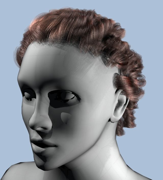
6
Fig. 6. Left: Azimuthal scattering geometry of the first three scattering modes (R,TT,TRT) within the normal plane for a fiber with circular cross section. The
relative azimuths ar denoted ϕR , ϕT T and ϕT RT . Here the projection of the angle of incidence onto the normal plane is γi0 and the angle of refraction γr0
respectively. Note that the outgoing ray leaves the fiber always at −hi . Right: Longitudinal scattering geometry of the first three scattering modes (R,TT,TRT)
at a dielectric fiber. Note that the outgoing inclinations θR ,θT T and θT RT always equal −θi . The difference of the longitudinal outgoing positions with
respect to incoming position si are denoted sR , sTT and sTRT .
or ϕTRT for the TRT-component. Here, the operator M maps Putting all geometric analysis together the geometry terms λ
the difference angle ϕo − ϕi to an interval (−π, π]: introduced in the previous section are:
α, −π < α ≤ π λR TT
s = 0; λs = sTT ; λTRT
s = sTRT
M [α] = α − 2π, π < α ≤ 2π (16) R TT
λh = λh = λh TRT
= −ho
α + 2π, −2π ≤ α ≤ −π
λR
ϕ = ϕ o + 2 arcsin ho
For the relative azimuths the following equations hold, cf. 0
λTT
ϕ = ϕo + M [π + 2 arcsin(ho ) − 2 arcsin(ho /n )]
Fig. 6 Left:
λTRT
ϕ = ϕo + 4 arcsin(ho /n0 ) − 2 arcsin ho (23)
ϕR = 2γi0 (17)
For smooth dielectric cylinders the R component gets attenu-
ϕTT = M [π + 2γi0 − 2γt0 ] (18)
ated by Fresnel reflectance only:
ϕTRT = 4γt0 − 2γi0 (19)
aR = Fresnel(n0 , ñ0 , γi0 ). (24)
Due to Bravais Law all azimuths are calculated from 2D-
0
scattering within the normal plane with help of a modified According to [2] the index n is used to calculate the re-
index of refraction flectance for perpendicular polarized light, whereas another
p index of refraction ñ0 = n2 /n0 is used for parallel polarized
0 n2 − sin2 θi light.
n =
cos θi For the two other modes (TT, TRT) a ray gets attenuated at
(instead of the relative refractive index n) and Snell’s Law each reflection rsp. refraction event. Hence for the correspond-
[2]. The projected (signed) angle of incidence light is denoted ing Fresnel factors FresnelTT and FresnelTRT the following
γi0 and equals arcsin hi . Its corresponding (signed) angle of equations hold:
refraction is γt0 = arcsin(hi /n0 ).
FresnelTT = (1 − aR )(1 − Fresnel(1/n0 , 1/ñ0 , γt0 )) (25)
Because rays entering the cylinder at a position si propagate
into longitudinal s-direction, they leave the fiber at another FresnelTRT = FresnelTT Fresnel(1/n0 , 1/ñ00 , γt0 ) (26)
positions sTT and sTRT respectively. In case of direct surface If a ray enters the cylinder, as is the case for both the TT
reflection (R-mode) the light is reflected at incoming position and TRT modes, absorption takes places. For homogenous
si . The two positions sTT and sTRT are directly related materials the attenuation only depends on the length of the
to the length covered by the ray inside the cylinder. For internal path—i.e. the absorption length—and the absorption
the TT component this length l can be calculated from its coefficient σ, which is a wave length dependent material
projection onto the normal plane ls , and the longitudinal angle parameter. For the TT component the absorption length equals
of refraction θt (see Fig. 6): l and a ray of the TRT mode covers twice this distance inside
ls 2r cos γt0 the cylinder. Note that the absorption length given in [2]
l= = (20) (which was l = (2 + 2 cos γt0 )/ cos θt ) is wrong.
cos θt cos θt
Hence the total attenuation factors with absorption are
with θt = − sgn(θi ) arccos((n0 /n) cos θi ). This length dou-
bles for rays of the TRT-mode. aTT = FresnelTT e−σ l , (27)
Therefore for the positions sTT and sTRT the following aTRT = FresnelTRT e−2σ l . (28)
holds:
p Note that higher order scattering can be analyzed in a
sTT = − sgn θi l2 − ls2 = ls tan θt (21) straight forward way, since analytical solutions for the cor-
sTRT = 2ls tan θt (22) responding geometry terms λ are available.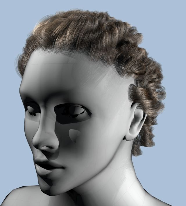
7

                                                                                    Notice that for the integration with respect to ξo one has to
                                                                                    take into account its transition of from zero to 2π properly.
                                                                                    Alternatively one gets the following equation by integration
                                                                                    with respect to h:
                                                                                                                     Z1
                                                                                                                D
                                                                                    dL̄o (ϕi , θi , ϕo , θo ) =           dLo (ho , ϕi , θi , ϕo , θo ) dho . (30)
                                                                                                                2
                                                                                                                     −1

                                                                                    The factor D amounts for the fact that the projected area to
Fig. 7. The left diagram shows the distribution of scattered light at a perfect     screen space is proportional to the width of a fiber.
smooth dielectric circular cylinder obtained with particle tracing. The intensity      Since we assume constant incident radiance Li (ϕi , θi ), dLo
of the scattered light is computed with respect to ξ and ∆s at the cylindric
shell: the darker the grey, the higher the outgoing flow through the surface. A     may be substituted by:
single light source is illuminating a small rectangular surface patch at s = 0
from direction ϕ = π and θ = 0.2. The direct surface reflection component             dLo (ϕi , θi , ho , ϕo , θo ) = cos2 θi Li (ϕi , θi )dϕi dθi dho
(R), the forward scattered component (TT) and the first order caustic (TRT)                 Z1 Z∞
are clearly and sharply visible. The right image shows the same scene but
a dielectric cylinder with volumetric scattering. As a consequence both TT                             fBFSDF (∆s, hi , ϕi , θi , ho , ϕo , θo ) d∆s dhi
and TRT components are blurred. Note that the structure of the scattering                      −1 −∞
distribution (i.e. the position of the peaks and their relative intensities) does
not change.                                                                                                                                                  (31)
                                                                                    which yields:
                                                                                                                  D
        VI. FAR F IELD A PPROXIMATION AND BCSDF                                     dL̄o (ϕo , θo , ϕi , θi ) =     Li (ϕi , θi ) cos2 θi dϕi dθi
                                                                                                                  2
   “Real world” filaments are typically very thin and long                                Z1 Z1 Z∞
structures. Hence, compared to its effective diameter both                                            fBFSDF (∆s, hi , ϕi , θi , ho , ϕo , θo ) d∆s dhi dho
viewing and lighting distances are typically very large. There-                          −1 −1 −∞
fore all surface patches along the normal plane have equal                                                                                                   (32)
(ϕo , θo ) and the fibers cross section is locally illuminated by
parallel light (of constant radiance) from a fixed direction                          This scattered radiance dL̄o is proportional to the incoming
(ϕi , θi ). Furthermore adjacent surface patches of the local                       curve irradiance dĒi :
minimum enclosing cylinder have nearly the same distance                                    dĒi (ϕi , θi ) := DLi (ϕi , θi ) cos2 θi dϕi dθi .              (33)
to both light source and observer.
   When rendering such a scene the screen space width of a                             Thus, a new bidirectional far-field scattering distribution
filament is less or in the order of magnitude of a single pixel.                    function for curves that assumes distant observer and distant
In this case fibers can be well approximated by curves having                       light sources can be defined. It relates the incoming curve
a cross section proportional to the diameter of the minimum                         irradiance to the averaged outgoing radiance along the the
enclosing cylinder D.                                                               width (curve radiance). We will call it fBCSDF (Bidirectional
   That allows us to introduce a simpler scattering formalism                       Curve Scattering Distribution Function):
to further reduce rendering complexity which we call far field                                                             dL̄o (ϕo , θo , L (ϕi , θi ))
approximation, cf. [3].                                                                fBCSDF (ϕi , θi , ϕo , θo ) :=                                    .   (34)
                                                                                                                                 dĒi (ϕi , θi )
   Using similar quantities as Marschner et al. [2] (curve
radiance and curve irradiance) we show how an appropriate                              By comparing the two equations (32) and (33) we obtain:
scattering function can be derived right from the BFSDF. The                                                                  Z1 Z1 Z∞
curve radiance dL̄o is the averaged outgoing radiance along                                                            1
                                                                                         fBCSDF (ϕi , θi , ϕo , θo ) =
the width of the fibers minimum enclosing cylinder times its                                                           2
                                                                                                                              −1 −1 −∞
effective diameter (Fig. 5).
                                                                                               fBFSDF (∆s, hi , ϕi , θi , ho , ϕo , θo ) d∆s dhi dho . (35)
   Assuming parallel light from direction (ϕi , θi ) being con-
stant over the width of a fiber this curve radiance can be                             Finally, in order to compute the total outgoing curve radi-
computed by averaging the outgoing radiance of all visible                          ance one has to integrate all incoming light over a sphere with
patches at so (over the width of the fiber) and weighting them                      respect to ϕi and θi :
with respect to their relative screen space coverage (projected
                                                                                                              Z2π Zπ/2
area to screen space) by a factor of cos (ξo − ϕo ):
                                                                                         L̄o (ϕo , θo ) = D
                                   ϕoZ+π/2                                                                    0 −π/2
                               D
dL̄o (ϕi , θi , ϕo , θo ) :=               cos (ξo − ϕo )                                      fBCSDF (ϕi , θi , ϕo , θo )Li (ϕi , θi ) cos2 θi dθi dϕi .(36)
                               π
                                ϕo −π/2
                                                                                   This equation matches the rendering integral given in [2,
      dLo (ϕi , θi , ξo , αo (θo , ho (ξo , ϕo )), βo (θo , ho (ξo , ϕo )))dξo . equation 1] in the specific context of hair rendering. Thus the
                                                                           (29) BCSDF is identical to the fiber scattering function very briefly
8

introduced in [2]. In contrast to [2] our derivation shows the               B. Curve Scattering with Locally Varying Incident Lighting
close connection between the BFSDF and the BCSDF. In our                        Although locally constant incident lighting may be assumed
formalism the BCSDF is just one specific approximation of                    in most cases of direct illumination, this situation may change
the BFSDF and can be computed directly from eqn. (35).                       in case of indirect illumination. For the sake of completeness
   Besides of the advantage of being less complex than the                   we give the result for curve scattering with varying lighting,
BFSDF the BCSDF can help to drastically reduce sampling                      too. For the rendering integral one obtains:
artifacts which would be introduced by subtle BFSDF detail
like very narrow scattering lobes. Nevertheless there are some               L̄o (ϕo , θo ) =
drawbacks. First of all local scattering effects are neglected                         Z∞ Z1 Z2π Zπ/2
which restricts the possible fields of application of the BCSDF                   D                   fvaryingCSDF Li cos2 θi dθi dϕi dhi d∆s
in case of close ups or indirect illumination. Furthermore, since                    −∞ −1 0 −π/2
the fiber properties are averaged over the width, the entire
                                                                                                                                              (39)
width (at least in the statistical average) has to be visible.
Otherwise undesired artifacts may occur. Finally the BCSDF                   with
is not adequate for computing indirect illumination due to
                                                                                    fvaryingCSDF (∆s, hi , ϕi , θi , ϕo , θo ) =
multiple fiber scattering in dense fiber clusters, since the far
field assumption is violated in this case.                                                  Z1
                                                                                          1
                                                                                               fBFSDF (∆s, hi , ϕi , θi , ho , ϕo , θo ) dho . (40)
                                                                                          2
                                                                                           −1
                VII. F URTHER S PECIAL C ASES
                                                                                        VIII. P REVIOUS SCATTERING MODELS
   Although a distant observer and distant light sources are
commonly assumed for rendering, there may be cases where                        Especially in the context of hair rendering several scattering
these two assumptions may be not valid. For those situations                 models for light scattering from fibers have been proposed. We
further approximations of the BFSDF are straight forward and                 now show, how they can be expressed in our notation which
can be derived similarly to the BCSDF. In particular we now                  for instance allows systematic derivations of further scattering
discuss the following two special cases:                                     functions basing on the corresponding BFSDF and BCSDF.
                                                                             Furthermore we discuss their physical plausibility.
  •    a close observer and locally constant incident lighting:
       near field scattering with constant incident lighting
  •    a distant observer with locally varying incident lighting:            A. Kajiya & Kay’s model
       curve scattering with locally varying incident lighting                  One of the first simple approaches to render hair, which is
                                                                             still very commonly used, was presented by Kajiya & Kay [1].
                                                                             It assumes a distant observer, since the outgoing radiance is
A. Near Field Scattering with Constant Incident Lighting                     constant over the width of a fiber and basically accounts for
                                                                             two scattering components: a scaled specular ad hoc Phong
   Although a BCSDF may be a good approximation for
                                                                             reflection at the surface of the fiber, centered over the specular
distant observers, it fails when it comes to close ups. Since
                                                                             cone and an additional colored diffuse component. The diffuse
the outgoing radiance is averaged with respect to the width
                                                                             coefficient Kdiffuse is obtained from averaging the outgoing
of a filament the intensity does not vary and local scattering
                                                                             radiance of a diffuse BRDF over the illuminated width of the
details can not be resolved. Now, if incident illumination can
                                                                             fiber, which produces significantly different results compared
be assumed locally constant (like in the case of distant light
                                                                             to the actual solution derived in section IX-A.1 (see Fig. 11).
sources) the outgoing radiance dL(ϕi , θi , ho , ϕo , θo ) can be
                                                                             The phenomenological Phong reflection fails to predict the
computed from eqn. 31. Integration with respect to incident
                                                                             correct intensities due to Fresnel reflectance (cf. section IX-
direction (ϕi ,θi ) yields:
                                                                             A.2).
                         Z2π Zπ/2                                               Kajiya & Kay’s model can be represented by a BCSDF as
  Lo (ho , ϕo , θo ) =              fnearfield Li cos2 θi dθi dϕi .   (37)   follows:
                                                                                    Kajiya & Kay           cosn (θo + θi )
                         0 −π/2                                                   fBCSDF         = KPhong                  + Kdiffuse .    (41)
                                                                                                                cos θi
with
                                                                             B. The model of Marschner et al. (2003)
  fnearfield (ϕi , θi , ho , ϕo , θo ) =                                        A much more sophisticated far field model for light scat-
           Z1 Z∞                                                             tering from hair fibers was proposed by Marschner et al. [2].
                   fBFSDF (∆s, hi , ϕi , θi , ho , ϕo , θo ) d∆sdhi .        It bases on significant measurements of light scattering from
           −1 −∞                                                             single hair filaments and implies again a distant observer and
                                                                      (38)   distant light sources. In [2] it is shown that all important fea-
                                                                             tures of light scattering from hairs can be basically explained
   A practical example of a near field scattering function for               by scattering from cylindrical dielectric fibers made of colored
dielectric fibers is given in section IX-B.                                  glass accounting for the first three scattering components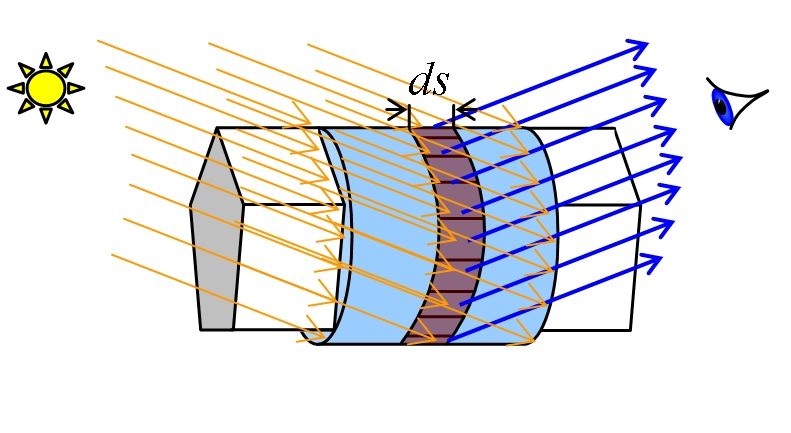
9

(R, TT, TRT) introduced in section V already. The BCSDF               one has:
representing the basic model of Marschner et al. (without                         aR (θd , hi )
                                                                        R
smoothing the caustic in the TRT component) can be directly            fBFSDF =
                                                                                    cos2 θd
derived from its underlying BFSDF, which is given by:                                                        θ
                                                                               δ(ho + hi )g(θo + θi − ∆θR , wR )δ(∆s)δ(ϕi − λϕ R )
       generatorMarschner
      fBFSDF              =
                                                                       Inserting this BFSDF into eqn. (35) for the corresponding
           δ(ho + hi )                      θ
                       (g(θo + θi − ∆θR , wR  )aR (θd , hi )          BCSDF yields:
             cos2 θd
             δ(∆s)δ(ϕi − λϕ R )                                          R           aR (θd , φ2 ) cos( φ2 )g(θo + θi − ∆θR , wR
                                                                                                                               θ
                                                                                                                                 )
                                                                        fBCSDF =                               2
                                                                                                                                   . (43)
             +g(θo + θi − ∆θTT , wTT θ
                                        )aTT (θd , hi )                                                   4 cos θd
                                                                      This equation matches the formula given in [2, equation 8]
             δ ∆s − λTT      δ(ϕi − λϕ TT )

                        s
                                     θ
                                                                      (for p = 0, inserting the ray density and attenuation factors).
              +g(θo + θi − ∆θTRT , wTRT )aTRT (θd , hi )                 Moreover, in [2] this basic BCSDF is extended to account
              δ(∆s − λTRT
                      s   )δ(ϕi − λTRT
                                    ϕ  )).               (42)         for elliptic fibers and to smooth singularities in a post pro-
                                                                      cessing step. Since the BCSDF is computed for a perfect
   This BFSDF can be seen as a generator for the basic
                                                                      smooth cylinder, there are azimuthal angles φc , for which
model proposed in [2]. Note that it matches the BFSDF for a
                                                                      the intensities of the TRT-components go to infinity. These
cylindric
     √     dielectric fiber with normalized Gaussians g(x, w) :=
                                                                      singularities (caustics) are unrealistic and have to be smoothed
1/( 2πw) exp(−x/(2w2 )) replacing the delta distributions
                                                                      out for real world fibers. The method used in [2] is to first
δθ . This accounts for the fact that no fiber is perfectly smooth,
                                                                      remove the caustics from the scattering distribution and to
and the light is scattered to a finite lobe around the perfect
                                                                      replace them by Gaussians (with roughly the same portion
specular cone. Additional shifts ∆θR,TT,TRT account for the
                                                                      of energy) centered over the caustics positions. Four different
tiled surface structure of hair fibers, which lead to shifted
                                                                      parameters are needed to control this caustic removal process.
specular cones compared to a perfect dielectric fiber. For
                                                                         Note that this rather awkward caustic handling for the
a better phenomenological match in [2] it is furthermore
                                                                      TRT component performed in [2] as well as a problematic
proposed to replace θi with θd = (θo − θi )/2. Hence this
                                                                      singularity in the ray density factor of the TT-component for
BFSDF is just a variation of eqn. (15) and the complex
                                                                      an index of refraction approaching the limit of one can be
derivation of the basic model (for a smooth fiber) given in
                                                                      avoided, if another BFSDF for non-smooth dielectric fibers is
[2] can be reduced to the following general recipe:
                                                                      used, cf. section IX-B.
   • Build a BFSDF by writing the scattering geometry in
                                                                         Usually hair has not a circular but has an elliptic cross
      terms of products of delta functions with geometry terms        section geometry. Since even mild eccentricities e especially
      λϕ and adding an additional attenuation factor.                 influence the azimuthal appearance of the TRT component,
   • Derive the corresponding BCSDF according to eqn. (35).
                                                                      this fact must not be neglected. In [2] the following simple
      All ray density factors given in [2] as well as multiple        approximation is proposed: Substitute an index n∗ for the
      scattering paths for the TRT-component are a direct             original refractive index n depending on ϕh = (ϕi + ϕo )/2
      consequence of the λϕ -terms within the δ-functions.            for the TRT-component as follows:
                                                 generatorMarschner
Note that for performing the integration of fBFSDF                                         1
in (35) symbolically, all delta functions of the form δ(ϕi −                  n∗ (ϕh ) =     ((n1 + n2 ) + cos(2ϕh )(n1 − n2 ))
                                                                                           2
λGϕ (ho )) have to be transformed to make them directly de-
pendent on the integration variable ho . This is achieved by          where
                                                                                      n1    = 2(n − 1)e2 − n + 2
applying the following rule:                                                          n2    = 2(n − 1)e−2 − n + 2.
    Z1                                    n−1
                                          X     f G (hio )
         f G (ho )δ(ϕi − λG
                          ϕ (ho ))dho =         dλG
                                                                       IX. E XAMPLES OF FURTHER A NALYTIC S OLUTIONS AND
                                                  ϕ     i
    −1                                    i=0 | dho (ho )|                              A PPROXIMATIONS
                                                                         In general it cannot be expected that for complex
with G ∈ {R, TT, TRT}. Here the expression f G (ho ) sub-
                                                                      BFSDF/BCSDF there are analytical solutions—a situation that
sumes all factors depending on ho (except the δ-function itself)
                                                                      is similar to the one for BSSRDF/BSDF. Nevertheless, in the
and hio denotes the i-th root of the expression ϕi − λG    ϕ (ho ).   following we derive analytical solutions or at least analytical
For both the R and the TT component there exists always
                                                                      approximations for some interesting special cases.
exactly one root. For the TRT component one needs a case
differentiation, since it exhibits either one or three roots. This
exactly matches the observation of [2] that one or three differ-      A. Opaque Circular Symmetric Fibers
ent paths for rays of the TRT component occur. Although it is            Perfectly opaque fibers with a circular cross section (like
basically possible to compute the roots hio for all components        wires) can be modeled by a generalized cylinder together
directly, it is—for the sake of efficiency—useful to apply the        with a BRDF characterizing its surface reflectance. For this
approximation given by [2, equation 10].                              common case we now show, how both BFSDF and BCSDF
   As an example we now have a look at the direct surface             can be derived. Since no internal light transport takes place,
reflection component (R-component). According to eqn. (42)            light is only reflected from a surface patch, if it is directly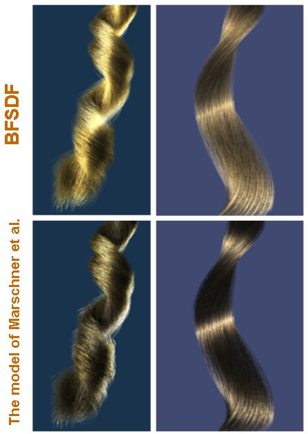
10

illuminated. Thus the BFSDF simply writes as a product of                      2) Fresnel Reflectance: A second very important feature of
the BRDF of the surface and two additional delta distributions              opaque fibers like metal wires or coated plastics is Fresnel
limiting the reflectance to a single surface patch:                         reflectance. We analyzed such a surface reflectance in the
                                                                            context of scattering from dielectric fibers in section V-A
               fBFSDF = fBRDF δ(ξo − ξi )δ(∆s)                       (44)   (R-component) and the corresponding BCSDF was already
or with respect to the other set of variables:                              derived in section VIII-B, cf. eqn. (43). In fact the BRDF
                                                                            is averaged over the width of a fiber, the BCSDF of a fiber
  fBFSDF = fBRDF δ(φ + arcsin ho − arcsin hi )δ(∆s) (45)                    with a narrow normalized reflection lobe BRDF (instead of a
with φ = M [ϕo −ϕi ] being the relative azimuth. To derive the              dirac delta distribution) can be very well approximated by this
BCSDF the complex (first) delta term has to be transformed                  BCSDF for smooth fibers. Some exemplary scenes rendered
into a form suitable for integration with respect to hi first.              with a combination of a Lambertian and a Fresnel BRDF
Applying the properties of Dirac distributions one obtains                  can be seen in Fig. 11. The BCSDF approximation produces
                                                                            very similar results compared to the precise BRDF (BFSDF)
           fBFSDF = fBRDF | cos(φ + arcsin ho )|                            solution, but required much less computation time.
               δ(hi − sin (φ + arcsin ho ))δ(∆s).                    (46)
   According to equation (35) for the BCSDF of a circular                   B. A Practical Parametric near field Shading Model for Di-
fiber mapped with an arbitrary BRDF the following holds:                    electric Fibers with Elliptical Cross Section

                            Z1 Z1 Z∞                                           In the following we derive a flexible and efficient near field
                        1                                                   shading model for dielectric fibers according to section VII-
           fBCSDF     =
                        2                                                   A. This model accurately reproduces the scattering pattern for
                            −1 −1 −∞                                        close ups but can be computed much more efficiently than
                fBRDF | cos (φ + arcsin ho )|                               particle tracing (or an equivalent) that was typically used to
                  δ(hi − sin (φ + arcsin ho ))                              capture the scattering pattern correctly.
                  δ(∆s)d∆sdhi dho                                    (47)      As a basis, we take the three component BFSDF given in
                  cos
                   Z φ                                                      eqn. (42) that was also used to derive the BCSDF correspond-
                1                                                           ing to the basic model proposed in [2], cf. section VIII-B.
              =       fBRDF |hi =sin (φ+arcsin ho )
                2                                                           Due to surface roughness and inhomogeneities inside the fiber
                      −1                                                    the scattering distribution gets blurred (spatial and angular
                      | cos (φ + arcsin ho )|dho                     (48)   blurring), cf. Fig. 7. In order to account for this effect we
Some exemplary results are shown in figure 11.                              replace all δ-distributions with special normalized Gaussians
   1) Lambertian Reflectance: Many analytical BRDFs in-                     g(I, x, w) := N (I, w) exp(−x/(2w2 )) with a normalization
                                                                                                      RI
clude a diffuse term accounting for Lambertian reflectance.                 factor of N (I, w) := 1/ exp(−x/(2w2 ))dx. The widths w
The BCSDF approximation for such a Lambertian BRDF                                                     −I
  Lambertian
(fBRDF       = kd ) component can be directly calculated from               of these Gaussians control the “strength of blurriness”. Fur-
eqn. (48):                                                                  thermore, we add a diffuse component approximating higher
                                                                            order scattering.
                            cos
                            Z φ
                       kd                                                      With these modifications we obtain the following more
      Lambertian
     fBCSDF          =           cos (φ + arcsin ho )dho             (49)   general BFSDF for non-smooth dielectric fibers:
                       2
                            −1                                                dielectric
                                                                             fBFSDF      =
with kd denoting the diffuse reflectance coefficient. To solve                     g(1, ho + hi , wh )     π                       θ
this integral we replace the integrand by the absolute value of                             2
                                                                                                       (g( , θo + θi − ∆θR , wR      )aR (θd , hi )
                                                                                         cos θd            2
its Taylor series expansion about ho = 0 up to an order of
                                                                                       g(∞, ∆s, ws )g(π, ϕi − λϕ R , wϕR )
two:
                                                                                          π                        θ
                     cos
                     Z φ                                                             +g( , θo + θi − ∆θTT , wTT        )aTT (θd , hi )
                kd                                h2o cos φ                               2
 Lambertian
fBCSDF        ≈            | cos φ − ho sin φ −             |dho .                   g ∞, ∆s − λTT                           TT
                                                                                                                                 , wϕTT )

                2                                     2                                             s , ws g(π, ϕi − λϕ
                     −1                                                                   π                          θ
                                                                                     +g( , θo + θi − ∆θTRT , wTRT        )aTRT (θd , hi )
                                                                     (50)                 2
                                                                                     g(∞, ∆s − λTRTs     , ws )g(π, ϕi − λTRT
                                                                                                                           ϕ     , wϕTRT ))
   For the resulting approximative BCSDF, which has a relative
error of less than five percent compared to the original, the                        +kd δ(∆s)                                                 (52)
following equations holds:                                                    Note that the awkward caustic handling done in [2] can
 Lambertian     kd                                                          be avoided by calculating the corresponding BCSDF out of
fBCSDF        ≈                                                              dielectric
                2                                                           fBFSDF      , cf. section VIII-B. Here, the appearance of the
      5                1        1       1                                   caustics is fully determined by the azimuthal blurring width
     | cos φ + cos2 φ − cos4 φ + sin φ − sin φ cos2 φ|.                       ϕ
      6                6        2       2                                   wTRT   . The more narrow this width is, the closer the caustic
                                                  (51)                      pattern matches the one of a smooth fiber. All azimuthal
11
TABLE I
S UMMARY OF ALL PARAMETERS OF THE NEAR FIELD SHADING MODEL .
notation meaning
∆θR,TT,TRT longitudinal shifts of the specular cones
θ
wR,TT,TRT widths for longitudinal blurring
ϕ
wR,TT,TRT widths for azimuthal blurring
n index of refraction
σ index of absorption Fig. 8. A simple example of a position dependent BSDF approximation for
kd diffuse coefficient the BFSDF. Left: BFSDF snapshot of a perfect dielectric cylinder (R,TT,TRT)
e eccentricity Right: Concentrating this BFSDF to the incident position gives a BSDF
depending on the incident offset hi on a flat ribbon.
scattering of such a BCSDF can be derived efficiently by
numerical integration in a preprocessing pass. The result is a BFSDF, which translate it to some position dependent BSDF
two dimensional lookup table with respect to θd and ϕ which and preserve subtle scattering details.
is then used for rendering and which replaces the complex
computations proposed in VIII-B. Some exemplary compar- A. BSDF Approximation of the BFSDF
isons between BFSDF and BCSDF-renderings are presented
in the appendix (Fig. 10). In most cases internal light transport is limited to a very
Assuming locally constant illumination a near field scatter- small region around the incident position. Furthermore, the
dielectric
ing function fnearfield can be derived from the BFSDF by diameter of a typical fiber is very small compared to other
dielectric
solving eqn. 38 in section VII-A for fBFSDF . Assuming a dimensions of a scene. Hence, concentrating the BFSDF to the
narrow width wh , i.e. a small spatial blurring, this approxi- infinitesimal surface patch in which incident light penetrates
mately yields: the fiber, introduces only very little inaccuracies (see Fig. 8).
This approach may be formalized by integrating an BFSDF
dielectric
fnearfield = 2kd with respect ∆s and ξo :
1 π θ
+ 2 (g( , θo + θi − ∆θR , wR )aR (θd , ho ) Z∞ Z2π
cos θd 2
fBSDF [hi ](ϕi , θi , ϕo , θo ) := fBFSDF dξo d∆s (54)
g(π, φ + 2 arcsin ho , wϕR )
π −∞ 0
θ
+g( , θo + θi − ∆θTT , wTT )aTT (θd , ho )
2 The result is some position dependent BSDF
g(π, φ + M [π + 2 arcsin ho − 2 arcsin (ho /n0 )], wϕTT ) fBSDF [hi ](ϕi , θi , ϕo , θo ) varying over the width of the
π θ fiber. With this approximation a fiber can be modeled very
+g( , θo + θi − ∆θTRT , wTRT )aTRT (θd , ho )
2 well by a primitive having the same effective cross section
g(π, φ + 4 arcsin (ho /n0 ) − 2 arcsin ho , wϕTRT )). (53) like the minimum enclosing cylinder, e.g. flat ribbons or half
cylinders always facing the light and camera.
This result can be directly used for shading of fibers with
a circular cross section. Although elliptic fibers could be
modeled by calculating the corresponding λ terms, we propose B. BCSDF as BSDF
to use the following more efficient approximation instead: If the BCSDF is used for rendering, its transformation to
Change the diameter of the primitive used for rendering (a half a BSDF is trivial: in fact nothing has to be changed. Only
cylinder or a flat polygon) according to the projected diameter diameter D has to be neglected in the rendering integral, if
and apply the first order approximation for mild eccentricities the fibers are modeled by primitives geometrically accounting
proposed in [2] (cf. section VIII-B). for their effective cross sections.
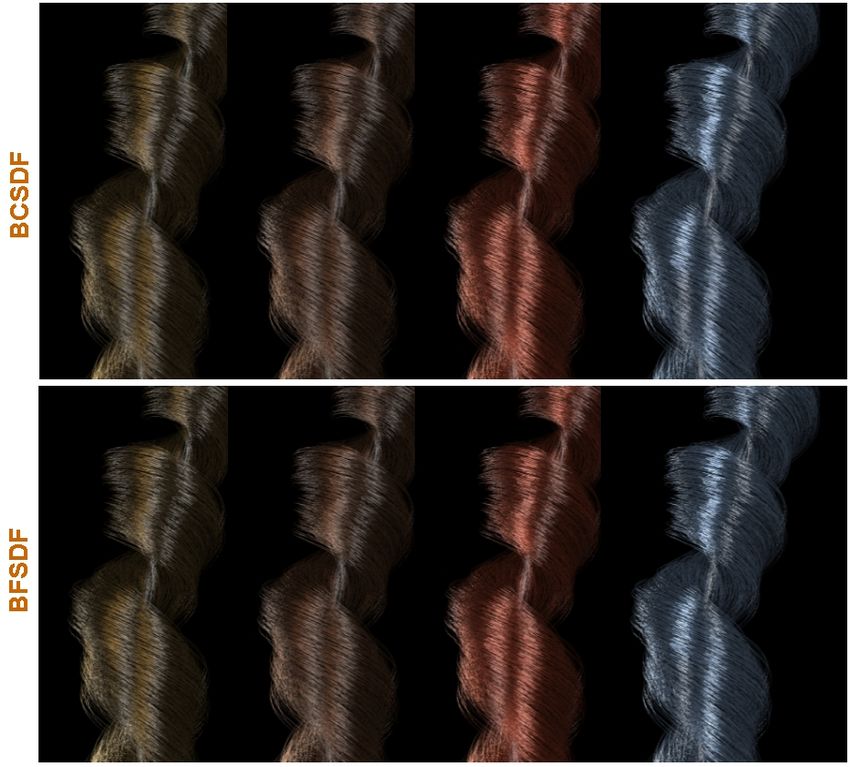
Results obtained with this model are given in the appendix
(Fig. 13, 14, 15, 11, 10). Notice especially the results shown
in Fig. 14, in which comparisons to photographs are given XI. I NDIRECT I LLUMINATION AND M ULTIPLE
showing how well the scattering patterns of the renderings are S CATTERING
matching the originals. For light colored fibers indirect illumination—mostly due
Interestingly, this near field shading model is computa- to multiple fiber scattering—significantly contributes to the
tionally less expensive than the far field model of [2]. It overall scattering distribution and must not be neglected. For
can be evaluated more than twice as fast (per call) com- an example we refer to [3], which addresses the importance
pared to an efficient reimplementation of this far field model. of global illumination in case of blond hair. A Monte Carlo
Furthermore an extension of the model to all higher order rendering of light blond hair is presented in Fig. 9.
scattering components is possible, since analytical expressions Because a BFSDF already comprises all internal light
for corresponding geometry terms λ are available. transport of a single filament, no further simulation of internal
scattering has to be performed. Therefore sampling a BFSDF
X. I NTEGRATION INTO E XISTING R ENDERING S YSTEMS for multiple filament scattering is more efficient than simu-
Existing rendering kernels can cope with BSDF and poly- lating the entire filament scattering—including internal light
gons only. Therefore we propose approximations of the transport–during rendering.12
However, although global illumination due to multiple Linear Basis Decomposition [26], clustering and factorization
fiber scattering can be basically accelerated by sampling the [27], [28], [29]) developed in the realm of BRDF and BTF
BFSDF—cf. section X— this direct approach may still be rendering.
impracticable with respect to rendering time. Another important challenge is the reconstruction of the
Especially in the field of interactive hair rendering several BFSDF or BCSDF from macroscopic image data, which
very efficient rendering techniques—such as deep or opacity frequently are more easily obtainable than systematic mea-
shadow maps and pixel blending—have been proposed to surements at the fiber level. We presume that using special
approximate effects of multiple fiber scattering [20], [21], modeling knowledge which is coded by the usage of a lower
[22], [23]. In a forthcoming publication we will show how dimensional scattering functions such as the BCSDF might
our theoretical framework can be applied to obtain physically be crucial for the practical solvability of inverse problems
based results using these techniques. involving the BFSDF.
Acknowledgements. We are grateful to the anonymous ref-
XII. C ONCLUSION AND F UTURE W ORK erees for many detailed suggestions. We would like to thank
R. Klein for the possibility to use a robot camera system for the
In this paper we derived a novel theoretical frame work
photographs given in Fig. 14, and to R. Sarlette and A. Hennes
for efficiently computing light scattering from filaments. In
for their technical support. The presented work is partially
contrast to previous approaches developed in the realm of hair
supported by Deutsche Forschungsgemeinschaft under grant
rendering it is much more flexible and can handle many types
We 1945/3-2.
of filaments and fibers like hair, fur, ropes and wires. Approxi-
mations for different levels of (geometrical) abstraction can be
derived in a straight forward way. Furthermore, our approach R EFERENCES
provides a firm basis for comparisons and classifications of
[1] J. T. Kajiya and T. L. Kay, “Rendering fur with three dimensional
filaments with respect to their scattering properties. The basic textures,” in Proceedings of the 16th annual conference on Computer
idea was to adopt basic radiometric concepts like BSSRDF graphics and interactive techniques. ACM Press, 1989, pp. 271–280.
and BSDF to the realm of fiber rendering. Although the [Online]. Available: http://doi.acm.org/10.1145/74333.74361
[2] S. R. Marschner, H. W. Jensen, M. Cammarano, S. Worley, and P. Han-
resulting radiance transfer functions are strictly speaking valid rahan, “Light scattering from human hair fibers,” ACM Transactions
for infinite fibers only, they can be seen as suitable local on Graphics, vol. 22, no. 3, pp. 780–791, 2003, SIGGRAPH 2003.
approximations. [Online]. Available: http://doi.acm.org/10.1145/882262.882345
[3] A. Zinke, G. Sobottka, and A. Weber, “Photo-realistic rendering of blond
Different types of scattering functions for filaments were de- hair,” in Vision, Modeling, and Visualization (VMV) 2004, B. Girod,
rived and parameterized with respect to the minimum enclos- M. Magnor, and H.-P. Seidel, Eds. Stanford, U.S.A.: IOS Press, Nov.
ing cylinder. The Bidirectional Fiber Scattering Distribution 2004, pp. 191–198.
[4] D. B. Goldman, “Fake fur rendering,” in SIGGRAPH ’97: Proceedings
Function (BFSDF) basically describes the radiance transfer at of the 24th annual conference on Computer graphics and interactive
this enclosing cylinder. It is an abstract optical property of a fil- techniques. New York, NY, USA: ACM Press, 1997, pp. 127–134.
ament which can be estimated by measurement, simulation or [Online]. Available: http://doi.acm.org/10.1145/258734.258807
[5] T.-Y. Kim, “Modeling, rendering and animating human hair,” PhD-
analysis of the scattering distribution of a single filament. The Thesis in Computer Science, University of Southern California, Decem-
BFSDF can be seen as the basis for all further approximations, ber 2002.
cf. Fig. 1. We believe that we have derived scattering functions [6] F. E. Nicodemus, J. C. Richmond, J. J. Hsia, I. W. Ginsberg, and
T. Limperis, Geometric considerations and nomenclature for reflectance,
for most of the special cases that will occur in practice. For ser. Monograph. National Bureau of Standards (US), 1977, vol. 161.
examples of rendering results based on various of the derived [7] H. W. Jensen, S. R. Marschner, M. Levoy, and P. Hanrahan, “A practical
scattering functions we refer to the appendix. model for subsurface light transport,” in SIGGRAPH ’01: Proceedings
of the 28th annual conference on Computer graphics and interactive
However, the theoretical analysis given in this paper should techniques. New York, NY, USA: ACM Press, 2001, pp. 511–518.
be seen as a starting point and further work is required [Online]. Available: http://doi.acm.org/10.1145/383259.383319
to investigate many important problems which arise in the [8] T. Mertens, J. Kautz, P. Bekaert, F. V. Reeth, and T. H.-P. Seidel,
“Efficient rendering of local subsurface scattering,” in Proceedings of
case of very complex “real world filaments” such as global the 11th Pacific Conference on Computer Graphics and Applications
illumination for fiber based geometries. As an example we 2003, 2003.
refer to [3] were the importance of multiple fiber scattering [9] K. J. Dana, B. van Ginneken, S. K. Nayar, and J. J. Koenderink,
“Reflectance and texture of real-world surfaces,” in IEEE Conference
for light colored hair was addressed. It plays an important on Computer Vision and Pattern Recognition, 1997, pp. 151–157.
role for the right perception of the hair color and must not be [10] V. L. Volevich, E. A. Kopylov, A. B. Khodulev, and O. A. Karpenko,
neglected (see also Fig. 9). Efficient compression strategies “The 7-th international conference on computer graphics and visualiza-
are needed, since the BFSDF is an eight dimensional function tion,” in Eurographics Symposium on Rendering, 1997.
[11] E. Groller, R. T. Rau, and W. Strasser, “Modeling and visualization of
such as the general BSSRDF. Moreover, if the BFSDF is given knitwear,” IEEE Transaction on Visualization and Computer Graphics,
in a purely numerical form, the four dimensional rendering vol. 1, no. 4, pp. 302–310, 1995.
integral itself is very costly to evaluate. Therefore, the BFSDF [12] Y.-Q. Xu, Y. Chen, S. Lin, H. Zhong, E. Wu, B. Guo, and H.-
Y. Shum, “Photorealistic rendering of knitwear using the lumislice,”
should be approximated by series of analytical functions which in SIGGRAPH ’01: Proceedings of the 28th annual conference on
can be efficiently integrated. Fortunately, many scattering Computer graphics and interactive techniques. New York, NY, USA:
distributions have very few intensity peaks which can be ACM Press/Addison-Wesley Publishing Co., 2001, pp. 391–398.
[13] N. Adabala, N. Magnenat-Thalmann, and G. Fei, “Real-time visualiza-
well approximated with existing compression schemes (e.g. tion of woven textiles,” in Publication of EUROSIS, J. C. Guerri, P. A,
Lafortune Lobes [24], Reflectance Field Polynomials [25], and C. A. Palau, Eds., 2003, pp. 502–508.You can also read