A Scalable and Production Ready Sky and Atmosphere Rendering Technique - Sébastien Hillaire
←
→
Page content transcription
If your browser does not render page correctly, please read the page content below

Eurographics Symposium on Rendering 2020                                                                                        Volume 39 (2020), Number 4
C. Dachsbacher and M. Pharr
(Guest Editors)

                                       A Scalable and Production Ready
                                   Sky and Atmosphere Rendering Technique

                                                                       Sébastien Hillaire 1
                                                                          1 Epic   Games, Inc

Figure 1: Rendered images of different atmospheric conditions and view points using the method presented in this article. Left to right:
ground views of an Earth-like daytime and Mars-like blue sunset, and space views of an Earth-like planet and an artistic vision of a tiny
planet.

         Abstract

         We present a physically based method to render the atmosphere of a planet from ground to space views. Our method is cheap to
         compute and, as compared to previous successful methods, does not require any high dimensional Lookup Tables (LUTs) and
         thus does not suffer from visual artifacts associated with them. We also propose a new approximation to evaluate light multiple
         scattering within the atmosphere in real time. We take a new look at what it means to render natural atmospheric effects,
         and propose a set of simple look up tables and parameterizations to render a sky and its aerial perspective. The atmosphere
         composition can change dynamically to match artistic visions and weather changes without requiring heavy LUT update. The
         complete technique can be used in real-time applications such as games, simulators or architecture pre-visualizations. The
         technique also scales from power-efficient mobile platforms up to PCs with high-end GPUs, and is also useful for accelerating
         path tracing.
         CCS Concepts
         • Computing methodologies → Rasterization; Ray tracing;

1. Introduction                                                                        tive from a physically based representation of the atmosphere’s par-
                                                                                       ticipating medium in real time. Our contributions in this paper are
Rendering natural phenomena is important for the visual simula-
                                                                                       the following:
tion of believable worlds. Atmosphere simulation and rendering
is important for applications requiring large open worlds with dy-
                                                                                       • We propose a sky and aerial perspective rendering technique re-
namic time of day, or viewing planets from space. Such applica-
                                                                                         lying on LUTs to evaluate expensive parts of the lighting integral
tions include games, architectural visualization and flight or space
                                                                                         at lower resolution while maintaining important visual features.
simulators. However, current methods have limitations: they are ei-
                                                                                       • We propose a novel way to evaluate the contribution of light mul-
ther restricted to views from the ground, can only represent a sin-
                                                                                         tiple scattering in the atmosphere. It can approximate an infinite
gle atmosphere type, require computationally expensive updates of
                                                                                         number of scattering orders and can also be used to accelerate
lookup tables (LUTs) when atmospheric properties are changed, or
                                                                                         path tracing.
can even exhibit visual artifacts.
                                                                                       • The technique supports dynamic time of day along with dynamic
   We present a method to render a planet’s sky and aerial perspec-                      updates of the atmospheric properties, all while rendering effi-

© 2020 The Author(s)
Computer Graphics Forum © 2020 The Eurographics Association and John
Wiley & Sons Ltd. Published by John Wiley & Sons Ltd.
S. Hillaire / Production Ready Atmosphere Rendering

  ciently on a wide range of devices, from a low-end Apple iPhone          of two values sampled form a LUT, visual artifacts can appear at
  6s to consoles and high-end gaming PCs.                                  the horizon due to resolution and parameterization precision is-
                                                                           sues. Yusov [Yus13] improved the situation through a better pa-
This method is used in Epic Games’ Unreal Engine† . In this pa-
                                                                           rameterization, which works well for Earth-like atmospheres. How-
per, we will be using photometric units (luminance/illuminance)
                                                                           ever, artifacts can still be visible in cases where the atmosphere is
instead of radiometric units (radiance/irradiance). This due to the
                                                                           denser. For each of these LUT models, multiscattering is achieved
prevalence of these terms in modern game engines [LdR14].
                                                                           by evaluating the in-scattering LUT iteratively: sampling the scat-
   After reviewing previous work in Section 2, we briefly describe         tered luminance from the previous scattering order LUT to evalu-
participating media rendering (with a focus on the atmospheric             ate the new one. When all are added together, this forms the final
case) in Section 3. The atmospheric material model used in this            in-scattering LUT with multiple scattering orders up to the itera-
paper is presented in Section 4, and our atmosphere rendering tech-        tion count. However, such LUTs are cumbersome to update when
nique is detailed in Section 5. Results and comparisons to a path-         a game needs to update its atmospheric properties, e.g. due to a
traced ground truth and to a previous model are discussed in Sec-          change in weather conditions or to match the art direction. It is
tion 6. Finally, we report on performance in Section 7 and conclude.       possible to time slice updates, but this will result in a visual delay
                                                                           between sun movement and sky color [Hil16]. LUT-based models
                                                                           have source code available online [Bru17b; Yus13] and have been
2. Previous work                                                           used successfully in several games [Hil16; dCK17; Bau19]. Go-
The first wave of sky rendering techniques were focused on ray             ing further, Bruneton [Bru17a] discussed all of those models ex-
marching the atmosphere from the view point. This is what Nishita          tensively, and compared their advantages and limitations.
et al. [NSTN93] first proposed as a method to render an atmosphere            One of the challenges when rendering an atmosphere is to repre-
from ground and space views. O’Neil [ONe07] proposed integrat-             sent volumetric shadowing due to hills and mountains. It is possi-
ing the in-scattered luminance per vertex for the sake of perfor-          ble to rely on epipolar lines [Yus13], shadow volumes [Bru17b],
mance, and to render the final sky color with the phase function           or a variant of shadow volumes extruding meshes from shadow
applied per pixel. Wenzel [Wen07] proposes the same idea but with          maps [Hoo16]. These techniques are fast but can only represent
in-scattered luminance stored in a texture that is updated over sev-       sharp shadows from opaque meshes. They will fail to render the
eral frames to amortize the cost. The major drawback of these mod-         soft shadows resulting from cloud participating media or sun disk
els is that they ignore the impact that light multiple scattering can      area light shadow penumbrae. This is an area where ray marching
have on the look of the sky.                                               still has a definite advantage in capturing such soft details.
   In order to reduce the cost of ray marching and include multiple
scattering, analytical models fitted on real measurements [PSS99]          3. Participating media rendering
or on reference generated using path tracing with spectral informa-
tion [HW12] have been proposed. These models are very fast to              Rendering participating media can be achieved using ray marching
evaluate and benefit from a simple parameterization: for example,          or path tracing. In both cases it involves using a material parameter-
a single turbidity value is used to represent the amount of aerosols       ization representing participating media as described by the radia-
in the air, resulting in a denser looking atmosphere. However, they        tive transfer equations [FWKH17]. In this framework, for a given
are limited to views from the ground and to the single atmosphere          position and considering a beam of light traveling in a direction,
type the parameters have been fitted to. For example, it is not pos-       per-wavelength absorption σa and scattering σs coefficients (m−1 )
sible to render the Mars sky when the model is fitted to the Earth         respectively represent the proportion of radiance absorbed, or scat-
sky.                                                                       tered, along a direction. The extinction coefficient σt = σa + σs
                                                                           represents the total amount of energy lost due to absorption and out-
   More advanced models have been proposed for rendering atmo-             scattering. Furthermore, when a scattering event occurs, the scatter
spheric effects with multiple scattering, for views ranging from the       direction needs to be decided based on a distribution represented
ground to space. Nishita [NDN96] proposed subdivision of the par-          by a phase function p of unit sr−1 .
ticipating medium into voxels, and the simulation of energy ex-
change between them. More affordable models that remove the                   Under strong real-time constraints, our approach relies on ray
voxel representation have been proposed: they store the result of
integrations that can be expensive to evaluate into lookup tables
that can be easily queried at run time on GPU. These LUTs can be                                                    Rtop                       Vis(li)=1
sampled per pixel at run time (according to view, sun and world                                                                       o
                                                                                                                                 t atm
information) to compute the transmittance and in-scattered lumi-                                                       ϴs
nance. Bruneton and Neyret [BN08] proposed a 4D LUT while                                                                                      Vis(li)=0
Elek [Ele09] discarded one dimension, effectively ignoring the                   c                           v              li
planet’s shadowing of the atmosphere that is visible when the sun                                 t                                        p
is just below the horizon. Because, in these models, in-scattering                                                  Rground
from the viewer to a mesh surface is evaluated as the subtraction
                                                                           Figure 2: Sketch illustrating how light single scattering within par-
                                                                           ticipating media is computed using Equation 1.
† https://www.unrealengine.com.

                                                                                                                                                 © 2020 The Author(s)
                                                                               Computer Graphics Forum © 2020 The Eurographics Association and John Wiley & Sons Ltd.
S. Hillaire / Production Ready Atmosphere Rendering

marching to first evaluate single scattering, as illustrated in Fig-                           Table 1: Coefficients of the different participating media compo-
ure 2. It assumes a set of Nlight directional lights, e.g. a sun and a                         nents constituting the Earth’s atmosphere.
moon. It also takes into account a virtual planet with a pure diffuse
response of the ground according to an albedo ρ. It involves inte-                              Type           Scattering (×10−6 m−1 )        Absorption (×10−6 m−1 )
grating the luminance L scattered toward an observer as a function
of the evaluation of the medium transmittance T , shadow factor S                               Rayleigh       σrs = 5.802, 13.558, 33.1      σra = 0
(Vis being shadowing from the planet and T from the atmosphere)                                 Mie            σms = 3.996                    σma = 4.40
as well as in-scattering Lscat along a path segment using                                       Ozone          σos = 0                        σoa = 0.650, 1.881, 0.085
                                                 Z kp−ck
       L(c, v) = T (c, p) Lo (p, v) +                      Lscat (c, c − tv, v) dt, (1)
                                                  t=0                                          • Mie theory represents the behavior of light when interacting
                        Rx
    T (xa , xb ) =e−            σt (x)kdxk                                                       with aerosols such as dust or pollution. Light can be scat-
                          b
                         x=xa                ,                                           (2)
                                                                                                 tered or absorbed. The phase function is approximated us-
                             Nlight
                                                                                         (3)     ing the Cornette-Shanks phase function [GK99] pm (θ, g) =
Lscat (c, x, v) =σs (x)       ∑ T (c, x) S(x, li ) p(v, li ) Ei ,                                  3    (1−g2 )(1+cos(θ)2 )
                             i=1                                                                  8π (2+g2 )(1+g2 −2g cos(θ))3/2   where g is the asymmetry parameter
       S(x, li ) =Vis(li ) T (x, x + tatmo li ),                                         (4)     in ]−1, 1[ determining the relative strength of forward and back-
                                                                                                 ward scattering. By default, g = 0.8. Please note that it is also
where c is the view camera position, v is the direction toward the
                                                                                                 appropriate to use the simpler Henyey-Greenstein phase func-
view for current position, p is the intersection surface point, tatmo
                                                                                                 tion.
the ray intersection distance with atmosphere top boundary, and
Lo the luminance at p, e.g. lighting on the virtual planet’s ground.                           For simplicity, we omit the parameters of these phase functions
li and Ei are the ith light direction and illuminance (considering                             in the remaining equations of this paper. We also represent an
                                                                                                                                 1
directional light sources).                                                                    isotropic phase function as pu = 4π .

   In this paper, we compare our new ray-marching approach with                                    Table 1 represents the scattering and absorption coefficients
results from a path tracer. Our path tracer is implemented on GPU                              of each component [Bru17a]. Participating media following the
to be able to visualize the result being refined in real time at in-                           Rayleigh and Mie theories have an altitude density distribution of
                                                                                                           −h                   −h
teractive frame rate. It implements Monte Carlo integration with                               d r (h) = e 8km and d m (h) = e 1.2km , respectively. Ozone is a spe-
delta tracking and importance sampling within participating me-                                cific component of the Earth that has been identified as impor-
dia [FWKH17]. It also leverages ratio tracking [NSJ] for faster                                tant for representing its atmosphere, since it is key to achieving
convergence when estimating transmittance. This is considered as                               sky-blue colors when the sun is at the horizon [Kut13]. Ozone
our ground truth.                                                                              does not contribute to scattering; it only absorbs light. Follow-
                                                                                               ing Bruneton [Bru17a; Bru17b], we represent the distribution as
                                                                                               a tent function of width 30km centered at altitude 25km, d o (h) =
4. Atmospheric model                                                                                         |h−25|
                                                                                               max(0, 1 − 15 ).
The atmospheric material model we use has been described in pre-
vious papers [BN08; Bru17a]. We focus on the simulation of tel-                                5. Our rendering method
luric planets, i.e. composed of a solid part made of rock or metal
we will call the ground. The planet’s ground and atmosphere top                                5.1. Discussion: observing the sky
boundary are represented by spheres with constant radii. The vari-                             We now describe the sky and aerial perspective visual components.
able h represents the altitude above the ground. In the case of the                            It helps to justify the choices we have made when building LUTs
Earth, the ground radius is Rground = 6360km and atmosphere top                                and the use of ray marching.
radius can be set to Rtop = 6460km, representing a participating
                                                                                                  Looking at Figure 3, it appears that an Earth-like sky is of low
media layer of 100km. We consider the ground to be a purely dif-
                                                                                               visual frequency, especially during daytime:
fuse material with a uniform albedo ρ = 0.3 [NAS]. When render-
ing the atmosphere’s participating media, we do not consider a wide                            • Rayleigh scattering is smooth.
spectral representation as in [Ele09]. Instead, we focus on typical                            • The halo around the sun due to the Mie scattering phase function
RGB-based rendering.                                                                             is also fairly smooth for realistic phase g values encountered in
                                                                                                 nature.
  An atmosphere consists of several components that are all im-
                                                                                               • Multiple scattering is a key component for rendering realistic
portant to consider in order to achieve the look of the Earth and
                                                                                                 images. As shown in Figure 3 (bottom row), it also has low visual
other planets:
                                                                                                 frequency.
• Rayleigh theory represents the behavior of light when interact-                              • Higher frequencies are visible toward the horizon because the
  ing with air molecules. We assume that light is never absorbed                                 atmosphere quickly gets denser there and thus light participates
  and can only scatter around [BN08]. The phase function describ-                                more. We must take that into account.
  ing the distribution of light directions after a scattering event is                            The main source of high frequencies within the atmosphere is
               3(1+cos(θ)2 )
   pr (θ) =    16π     , where θ is the angle between incident and                             due to the planet’s shadow (at sunset) and shadows from moun-
   outgoing scattering directions.                                                             tains occluding single scattering events in Equation 3. The solution

© 2020 The Author(s)
Computer Graphics Forum © 2020 The Eurographics Association and John Wiley & Sons Ltd.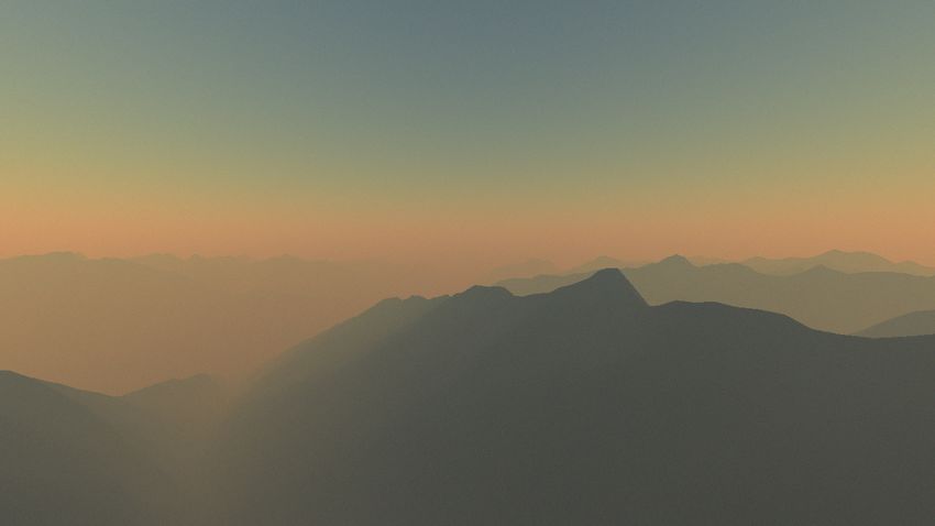
S. Hillaire / Production Ready Atmosphere Rendering

                                                                               π/2
                                                                                                                                                     Sky

                                                                                  Latitude
                                                                                 0
                                                                                                                                                  Horizon

                                                                                                                                               Planet ground

                                                                              -π/2
                                                                                                                   Longitude

Figure 3: Top: a scene with sun, sky and aerial perspective without           Figure 4: The Sky-View LUT during daytime. The sun direction can
(left) and with (right) volumetric shadows. Bottom: images present            be seen on the left side, where Mie scattering happens.
a ground view when multiple scattering is evaluated (right) or not
(left). Note: global illumination on the terrain is disabled to make
observations more visible.

                                                                              Linear latitude parameterisation

we propose can render the atmosphere with two modes: volumetric
shadow disabled, i.e. taking advantage of the Sky-View LUT for
faster rendering (see Section 5.3) or enabled, i.e. for a more accu-          Non-linear latitude parameterisation
rate but also more expensive render (see Section 7).
                                                                              Figure 5: The non-linear parameterization of the Sky-View LUT
                                                                              helps to concentrate texel details at the horizon, where it visually
5.2. Transmittance LUT                                                        matters.
When ray marching is executed to integrate Lscat , the shadowing
term T — representing the atmospheric medium casting onto it-
self — must be evaluated. However, executing a second ray march                  This effectively compresses more pixels close to the horizon and
toward the sun for each single scattering sample would be expen-              improves the amount of detail present there. It also helps hide the
sive. To accelerate that, the function T is stored as a LUT using             fact that the atmosphere is rendered at a lower resolution, as shown
the same representation described in Section 4 of Bruneton and                in Figure 5. The sun disk is not rendered as part of that texture be-
Neyret [BN08].                                                                cause of the low resolution and the non linear mapping. It is com-
                                                                              posited after applying the Sky-View LUT.
5.3. Sky-View LUT
Given the overall low frequency of the participating media consti-            5.4. Aerial Perspective LUT
tuting the atmosphere (see Section 5.1), it should be enough to ray           When rendering a scene, the aerial perspective effects on opaque
march it with a low number of samples. However, doing so for each             structures (e.g. terrain, mountains, and buildings) and translu-
pixel can be expensive, especially at high resolution such as 4K or           cent elements (e.g. glass, fire, or other participating media such
8K. Given the overall low visual frequency of the sky, we should              as clouds) must be rendered for consistency. Thus, similar to
be able to render the sky at a lower resolution and upsample it to            Hillaire [Hil16], we evaluate in-scattering and transmittance to-
higher resolution afterward.                                                  wards the camera in a volume texture fit to the view camera frustum
   For a given point of view, we propose to render the distant sky            (see Figure 6). In-scattering is stored in the RGB channels while the
into a latitude/longitude texture, oriented with respect to the cam-          transmittance is stored in the A channel, as the mean of the wave-
era local up vector on the planet’s ground for the horizon to al-             length dependent RGB transmittance.
ways be a horizontal line within it. For an example of this, see                 The default resolution used in our case is 32 × 32 over the screen
Figure 4, where the upper part represents the sky and the lower               and 32 depth slices over a depth range of 32 kilometers, which is
part the virtual planet ground, with the horizon in the middle.               enough for most applications and games. This is the case for Epic
In Section 5.1, we mentioned that higher-frequency visual fea-                Games’ Fortnite‡ , having a world map size of 3km2 with an Earth-
tures are visible toward the horizon. In order to help better rep-            like stylized atmosphere setup. If the planet’s atmosphere is really
resent those, we apply a non-linear transformation to the latitude l          dense up to a point where distant objects are less visible, then the
when computing the texture coordinate v ∈ [0, 1] that will compress
more texels near the horizon.
                         q       A simple quadratic curve is used:
                            |l|                                               ‡ https://www.epicgames.com/fortnite.
v = 0.5 + 0.5 ∗ sign(l) ∗   π/2
                                ,   with l ∈ [−π/2, π/2].

                                                                                                                                                    © 2020 The Author(s)
                                                                                  Computer Graphics Forum © 2020 The Eurographics Association and John Wiley & Sons Ltd.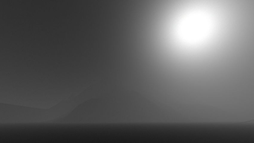
S. Hillaire / Production Ready Atmosphere Rendering

depth range can be brought back closer to the view point, in order                         resulting from higher-order light scattering events around a sam-
to increase accuracy over short range.                                                     ple point can be approximated by integrating the in-scattered light
                                                                                           over the surrounding sphere, from neighboring points that receive
   The aerial perspective volume texture is applied on opaque ob-
                                                                                           the same illuminance E, while taking into account the transmittance
jects as a post process after lighting is evaluated, at the same time as
                                                                                           between those points. This idea of using global in-scattered illumi-
the Sky-View LUT is applied on screen. For transparent elements
                                                                                           nance E as the input to evaluate multiple scattering using the local
in a forward-rendering pipeline, we apply aerial perspective at the
                                                                                           material data is inspired by the dual scattering method approximat-
per-vertex level. This is because transparent elements are usually
                                                                                           ing light multiple scattering in hair [ZYWK08].
small in screen space relative to atmospheric visual variations.
                                                                                              When light scatters around in a medium, the distribution of scat-
                                                                                           tering directions quickly becomes isotropic [JMLH01; Yan97]. For
5.5. Multiple scattering LUT                                                               the sake of performance, we would like our multiple scattering
As described in Section 2, previous atmospheric rendering tech-                            LUT to have a low dimensionality. To this aim, we assume that
niques [BN08; Ele09; Yus13] rely on iterative methods to update                            light bouncing around for scattering orders greater than or equal
3D or 4D LUTs, with one iteration per scattering order. This is an                         to 2 will be achieved according to an isotropic phase function, i.e.
acceptable solution when rendering Earth-like atmospheres where                            without any preferred directions. As such, we will ignore the Mie
only a multiple scattering order of 5 is required to reach realistic                       and Rayleigh phase function setup as part of the multiple scattering
sky visuals. However, it quickly becomes impractical when render-                          approximation. We feel that this an acceptable fit considering that
ing thicker atmosphere, i.e. when higher scattering orders are im-                         the Rayleigh phase function is already smooth. In order to get a bet-
portant for the atmosphere’s look and it is thus necessary to iterate                      ter intuition about the approximation for the case of Mie scattering,
many times over the LUTs. Practically, this operation of complexity                        we refer the reader to the analysis of BSDF shape with respect to
O(n) (where n is the scattering order) is computationally too heavy.                       scattering orders conducted by Bouthors [Bou08].
This is especially the case when artists are constantly updating at-                         Furthermore, it has been shown that a correlation exists be-
mospheric properties to match art direction or weather changes at                          tween second order scattered luminance and further scattering or-
different times of day. The computation can be time sliced [Hil16]                         ders [HG13]. Thus we propose to evaluate the multiple scattering
but this will result in update delays, which can impact the reactiv-                       contribution in the atmosphere as a function of the second order of
ity of other systems such as global illumination or reflection cube                        scattered luminance arriving at each sample point.
maps captured in real time.
                                                                                             We build our method from these previous results, and it will be
   Our goal is to propose a cheaper and instant O(1) method that is                        described in depth in Section 5.5.3. Here is a summary of it, to-
independent of the scattering order, to be able to evaluate the light                      gether with its approximations when evaluating multiple scattering:
multiple scattering contribution each and every frame without any
delay. Maintaining correctness and believability for a wide range                          • Scattering events with order greater or equal to 2 are executed
of atmosphere setups is also a requirement, as well as being able                            using an isotropic phase function pu .
to render atmospheres across a range of devices (from mobile to                            • All points within the neighborhood of the position we currently
high-end PC). Last but not least, we want our approach to rely on                            shade receive the same amount of second order scattered light.
a physically based participating media parametrization and to be                           • We compute the second scattering order contribution L2nd order
energy conserving.
                                                                                                       Colors scaled x50                 Colors scaled x1
5.5.1. Building an intuition about our approximation                                      Top

Given the overall large scale, long mean free path, and smooth dis-
                                                                                            Altitude

tribution of participating media in the atmosphere, it can be consid-
ered that the illuminance E reaching a point in space is the same for
all points within a large area around it. Thus integrating luminance

                                                                                               0       Sun / Zenith angle   π

                                                                                           Figure 7: Visualization of Equation 10 Ψms stored in multiple scat-
                                                                                           tering LUTs. Left: the LUT for the Earth setup. It is broadly uni-
                                                                                           form, and scattering dominates over transmittance. Right: 50 times
                                                                                           denser air, causing Rayleigh scattering with a modified distribu-
                                                                                                              h
                                                                                           tion d r (h) = e 20km . The contribution of multiple scattering increases
                                                                                           with the density of the medium, until transmittance overtakes it, re-
Figure 6: The camera frustum aerial perspective LUT. This is a                             sulting in a drastic reduction of light reaching the ground. This is
visualization of in-scattering for a few slices.                                           especially true when the sun is close to the horizon.

© 2020 The Author(s)
Computer Graphics Forum © 2020 The Eurographics Association and John Wiley & Sons Ltd.
S. Hillaire / Production Ready Atmosphere Rendering

  and a transfer function fms (taking into account transmittance                 medium around and towards the currently shaded sample at posi-
  and medium variation along altitude) from the participating me-                tion xs as
  dia around the position we currently shade.                                                                  Z
• Finally, we compute the multiple scattering contribution Ψms                                         fms =       L f (xs , −ω) pu dω,                                (7)
                                                                                                               Ω4π
  from these factors, simulating the infinite scattering of the sec-                                          Z kp−xk
  ond order light contribution isotropically with respect to the                                 L f (x, v) =           σs (x) T (x, x − tv) 1 dt.                     (8)
  transfer function from neighborhood points, back to the currently                                            t=0
  shaded position.                                                               This is illustrated in Figure 8 (right). The directional integration
• Visibility Vis is ignored when evaluating multiple scattering.                 over the sphere is computed as fms , where L f is integrated along
  This relies on the fact that light will scatter around mountains               each ray using Equation 8. It is important to skip the sampling of
  anyway, e.g. the impact of visibility is low for natural atmo-                 the shadowing term S and phase function in this equation because
  spheres with a large mean free path.                                           it is already accounted for when evaluating L2nd order . Thus fms is a
                                                                                 unitless normalized transfer factor of the energy integrated around
5.5.2. LUT parameterization                                                      and towards xs , in the range [0, 1] . To help respect that range, it
                                                                                 is recommended to use the analytical solution to the integration of
For any point in space, we want to be able to store and query the                Equation 8 as proposed by Hillaire [Hil15].
isotropic multiple scattering contribution to luminance from a LUT.                 As mentioned above, we assume that light reaching any point
Given that we consider the virtual planet to be a perfect sphere, the            around xs is the same as that reaching xs itself for scattering orders
multiple scattering contribution to be isotropic, and the distribution           greater than to 2. We can use this low spatial variation assump-
of medium in the atmosphere to only vary based on altitude, we                   tion to evaluate the multiple scattering contribution analytically.
represent this LUT as a small 2D texture. The u, v parameterization              Inspired by the dual-scattering approach [ZYWK08], we approx-
in [0, 1]2 is:                                                                   imate the infinite multiple scattering light contribution factor Fms
• u = 0.5 + 0.5 cos(θs ), where θs is the sun zenith angle and ωs                as a geometric series infinite sum
  represents its direction.                                                                                                                       1
                     h−R                                                                        Fms =1 + fms + f2ms + f3ms + ... =                     .               (9)
• v = max(0, min( Rtop −Rground
                           ground
                                  , 1)), where the sample position xs is                                                                       1 − fms
  at altitude h.
                                                                                    Finally, the total contribution of a directional light with an infi-
An example of such LUTs and their parameterization can be seen                   nite number of scattering orders can be evaluated as
in Figure 7.
                                                                                                               Ψms =L2nd order Fms ,                                 (10)
5.5.3. High scattering order LUT evaluation                                      where the second order scattering contribution L2nd order is ampli-
                                                                                 fied by the multiple scattering transfer function Fms . The transfer
Considering a sample point at position xs and altitude h, we inte-               function Ψms (unit sr−1 ) is thus simply multiplied with any direc-
grate the second order scattered luminance L2nd order towards point              tional light illuminance (Lux as cd.sr.m−2 ) to retrieve the multiple
xs (as illustrated in Figure 8 (left)) using                                     scattering contribution to a pixel as luminance (cd.m−2 ). Ψms is
                  Z                                                              stored in the multiple scattering LUT. For an atmosphere material
   L2nd order =          L0 (xs , −ω) pu dω,                            (5)      setup, this LUT is valid for any point of view and light direction
                   Ω4π
                                                                                 around the planet.
     L0 (x, v) = T (x, p) Lo (p, v) +
                  Z kp−xk                                               (6)        To conclude, the light scattering Equation 3 can now be aug-
                             σs (x) T (x, x − tv) S(x, ωs ) pu EI dt.            mented with our multiple scattering approximation, which gives
                   t=0
                                                                                                                Nlight
In Equation 6, the L0 term evaluates the luminance contribution                    Lscat (c, x, v) = σs (x)      ∑ (T (c, x) S(x, li )p(v, li ) + Ψms )Ei .          (11)
from a single directional light with illuminance EI and with a di-                                              i=1
rection ωs , for a position xs matching the current LUT entry being              This simplification avoids a reliance on an iterative method to eval-
built. It also contains the luminance contribution reflected from the            uate the multiple scattering contribution within the atmosphere. For
ground through Lo (diffuse response according to albedo). L2nd order             our real-time use case, the integration of fms and L2nd order over the
should give the second order scattered light towards point xs as lu-             unit sphere is achieved using 64 uniformly distributed directions.
minance. But it is evaluated using EI : it is a placeholder for what             For more performance details, please refer to Section 7.
should be light illuminance Ei . Though in this case it is a unitless
factor EI = 1 to ensure that L2nd order does not return a luminance
value, but instead acts as a transfer function of unit sr−1 , only re-           6. Results
turning luminance when later multiplied with the actual directional
                                                                                 We validate our approach to atmosphere rendering by comparing it
light illuminance. In Equation 5, Lo is also evaluated using EI but
                                                                                 to two state of the art techniques: the model proposed by Brune-
we kept this out for simplicity.
                                                                                 ton [Bru17a] and a volumetric path tracer. We compare various
   Secondly, we integrate a unitless factor fms representing the                 scenarios and give the image root mean square error (RMSE) for
transfer of energy that would occur from all of the atmospheric                  each of the R, G and B channels as compared to the ground truth

                                                                                                                                                       © 2020 The Author(s)
                                                                                     Computer Graphics Forum © 2020 The Eurographics Association and John Wiley & Sons Ltd.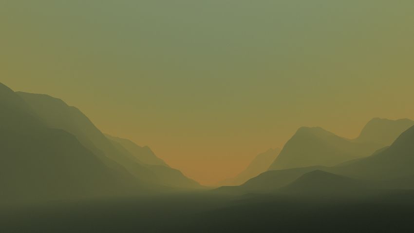
S. Hillaire / Production Ready Atmosphere Rendering
E� = 1 Lf(x,v) fms
T(xs,x) dω dω
Lf(x,v) dω Lf(x,v) dω fms
L'(s,v) fms
dω
L'(s,v)
T(xs,x)
L'(s,v)
dω xs fms
dω
dω xs
2
fms
dω
...
dω T(xs,x) dω
fms fms
Lf(x,v) dω Lf(x,v) dω
dω dω
xs
L2ndorder Lf(x,v) fms
Figure 8: Sketch presenting on the left how L2nd order is computed from single scattering L0 and, on the right, how Fms approximates multiple
scattering bounces using a normalized transfer function fms , corresponding to Equation 7, and assuming a sample point neighborhood
receive the same amount of energy as the sample point itself, corresponding to Equation 9.
Bruneton Ours Path traced reference
path tracer. We show the results on a planet with a terrain using a
pure-black albedo, and without sun disk, so as not to influence the
RMSE measure. The code for this application is open source§ . Earth
Firstly, we verify that our model can faithfully render the Earth’s
atmosphere — see Figure 9. We present views using single scat-
Mars like
tering only in order to show the difference when multiple scatter-
ing is taken into account. It also shows the three models: Brune-
ton (B), our model (O) and the reference path tracer (P). At day-
time, (B) and (O) RSME are respectively (1.43, 2.28, 6.07).10−3
Tiny planet
and (0.94, 1.74, 5.07).10−3 — both very close to the reference (P).
For the sunset case, it is important to note that (B) does not faith-
fully represent the orange color propagated by Mie scattering. This
is because we use a single RGBA 4D scattering LUT, where A
represents colorless Mie scattering, rather than a solution requiring Figure 10: Space view rendering of different planets: Earth, Mars
two RGB 4D scattering LUTs. This is the typical setup used in real- like and a fictional tiny planet with a thick and dense atmosphere.
time applications in order to allocate less memory and to increase
performance (only 1 scattering LUT needs to be updated and it re-
§ https://github.com/sebh/UnrealEngineSkyAtmosphere.
quires less bandwidth to fetch LUT data). The Mie scattering color
is recovered using the trick discussed in Section 4 of Bruneton and
Neyret [BN08]. It is also interesting to note that both models are
Path traced reference Bruneton Ours Path traced reference able to reproduce the pale scattering color visible in the shadow
Single scattering Multiple scattering
cast by the Earth within the atmosphere — see bottom of Figure 9.
Daytime
We also compare the accuracy of those models to achieve
space views, see Figure 10. Both (B) and (O) models are able
to faithfully reproduce the Earth, with respective RSMEs of
Sunset
(0.58, 0.67, 1.61).10−3 and (0.95, 0.85, 1.23).10−3 , as well as a
Mars-like planet atmosphere, RSMEs of (0.87, 0.97, 0.94).10−3
and (1.99, 0.91, 0.56).10−3 . When it comes to artistic tiny plan-
150° view
ets with thick and dense atmospheres, it appears that (B) is not able
to reproduce the volumetric shadowing from the planet’s solid core
with high quality. This is due to the LUT parameterization, which
Figure 9: Rendering Earth’s atmosphere with different techniques results in a lack of accuracy for small planets inherently featur-
under different conditions: daytime, sunset, and a 150 degree view ing a high ground-surface curvature. This limitation of model (B)
of the sky with sun below the horizon revealing the shadow cast by could be lifted by increasing the 4D light scattering LUT resolu-
the Earth within the atmosphere. Note: various exposures are used tion, adding additional memory and computational costs.
in this figure to ensute that visuals are readable.
For Earth’s atmosphere, it has been reported that computing scat-
© 2020 The Author(s)
Computer Graphics Forum © 2020 The Eurographics Association and John Wiley & Sons Ltd.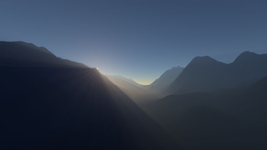
S. Hillaire / Production Ready Atmosphere Rendering

                                                Daytime                                                                                     Sunset
    Path traced reference - Single scatter             Ours                                         Path traced reference - Single scatter       Ours

    Path traced reference - depth=5                    Path traced reference - depth=40             Path traced reference - depth=5              Path traced reference - depth=40

    Bruneton 5 iterations                              Bruneton 40 iterations                       Bruneton 5 iterations                        Bruneton 40 iterations

 Figure 11: Daytime on ground (left) and sunset up in the atmosphere (right) views demonstrating that it is important to consider higher
 scattering orders for denser participating media. Our approach is the only non-iterative technique that can approximate the ground truth.

               Mie scattering (g = 0.0)   Mie scattering (g = 0.8)   Earth atmosphere 55x thicker
                                                                                                      • When using very high scattering coefficients, the hue can be lost
                                                                                                        or even start to drift as compared to the ground truth.
      Ours

                                                                                                      • We assume that the light scattering direction is isotropic right af-
                                                                                                        ter the second bounce. This is in fact an approximation, which is
                                                                                                        confirmed by a comparison between our model and the reference
(depth=100)
Path tracing

                                                                                                        path tracer. For Mie scattering only, with g = 0.0 and g = 0.8,
                                                                                                        RMSE is 0.0058 and 0.039, respectively.

                                                                                                      7. Performance and Discussion
 Figure 12: Limitations of our method when the atmosphere be-
 comes dense. Left and middle: the larger the phase g value, the less                                 On a PC equipped with an NVIDIA 1080, the final on-screen ren-
 accurate it is. Right: a dense atmosphere can result in a different                                  dering of the sky and atmospheric perspective is 0.14 milliseconds
 multiple-scattering color.                                                                           (ms) considering the daytime situation depicted in Figure 9. More
                                                                                                      detailed timings and the properties of the LUTs generated by our
                                                                                                      method are provided in Table 2. In the end, the total render time
                                                                                                      is 0.31 ms for a resolution of 1280 × 720. For the same view, the
 tering only up to the 5th order was enough to capture most of the en-                                Bruneton model [BN08] renders in 0.22ms, but this is without all
 ergy [BN08], and we have been able to confirm this by observation.                                   the LUTs being updated. Updating all the LUTs using the code pro-
 However, when control is given to artists to setup an atmosphere,                                    vided [Bru17b] costs 250ms, where 99% of this cost comes from
 the atmosphere may get denser and it then becomes important to                                       the many iterations required to estimate multiple scattering. As al-
 account for higher scattering orders. While our new model (O) au-                                    ready shown by Hillaire [Hil16], it is possible to time slice the up-
 tomatically takes that into account, it is not the case for model (B).                               date over several frames. However, latency would increase when
 In this case, there must be as many iterations as there are scattering                               evaluating high scattering orders, and it would take a long time be-
 orders that need to be evaluated, which quickly becomes impracti-                                    fore any result would be available on screen.
 cal, even with time slicing. Figure 11 demonstrates that for denser                                     When viewing the planet from space, as seen in Figure 10, the
 atmospheres, higher-order scattering is crucial for faithfully pro-                                  Sky-View LUT described in Section 5.3 becomes less accurate be-
 ducing the correct atmospheric color. Our model is able to repre-                                    cause a large part of it is wasted to render empty space. In this
 sent such behavior, while model (B) fails to converge to the correct                                 case, we seamlessly switch to simple ray marching on screen. The
 color for higher scattering orders, and even explodes numerically                                    planet and atmosphere render time then becomes more expensive
 (Figure 11 (right)). This is likely due to precision issues when sam-                                (0.33ms) resulting in a total rendering cost of 0.5ms. But this is of-
 pling the LUTs, even though we are using a 32 bit float represen-                                    ten acceptable as planetary views focus on the planet itself, so the
 tation for the model (B) scattering LUT, instead of a 16 bit float                                   rendering budget is likely higher.
 representation that is enough for model (O).
                                                                                                         Our technique can scale from desktop PC to relatively old Apple
   As shown in Figure 12, the new model (O) does have a few issues                                    iPhone 6s mobile hardware. In this case, LUT resolution and sam-
 worth mentioning, each of which are due to the multiple scattering                                   ple count can be scaled down without a huge impact on the result-
 approximation:                                                                                       ing visuals. Our setup and performance differences are illustrated

                                                                                                                                                                            © 2020 The Author(s)
                                                                                                          Computer Graphics Forum © 2020 The Eurographics Association and John Wiley & Sons Ltd.
S. Hillaire / Production Ready Atmosphere Rendering

                     PC                                         Mobile                         Path traced reference   Path traced reference - depth=5   Our

                                                                                           Figure 14: Volumetric shadows from the atmosphere, from left to
                                                                                           right: path-traced single scattering, path-traced multiple scattering
                                                                                           (depth = 5) and our real-time approach using ray marching and
                                                                                           cascaded shadow maps.

Figure 13: Visual comparison between PC (NVIDIA 1080) and mo-                              and reprojection can automatically be achieved via a temporal anti-
bile (iPhone 6s) rendering of the atmosphere. Only the sky is vis-                         aliasing (TAA) approach [Kar14]. This is illustrated in Figure 14.
ible at daytime (top) and at sunset with 5× higher Rayleigh scat-                          Using such an approach requires a sample count that is content de-
tering coefficients (bottom). Bloom, color grading and other post-                         pendent. In this example, we use 32 samples, which causes the sky
processing effects have been disabled.                                                     and atmosphere rendering time to go up to 1.0ms. To reduce this
                                                                                           cost, it is also possible to trace at a lower resolution and temporally
                                                                                           reproject and upsample the result. This has already been used, with
                                                                                           great results, in a few game engines [Bau19; EPI18]. Results with
in Table 2, while changes in visuals are presented in Figure 13. Vi-
                                                                                           volumetric shadows are shown in Figure 1.
sual differences, due to lower LUT quality, are not noticeable to the
naked eye. Please note that we do maintain a similar transmittance                            Furthermore, the multiple-scattering LUT we propose can also
LUT on both platforms as it is important for ensuring a matching                           accelerate path tracing of the atmosphere participating media, if
look. Its quality could be further reduced on mobile if more visual                        the approximations described in Section 5.5 and Figure 12 are ac-
differences can be traded for performance. For Epic Games’ Fort-                           ceptable. In this case, only single scattering events need to be sam-
nite, the total sky rendering cost was roughly 1ms on iPhone 6s.                           pled, e.g. using delta tracking [FWKH17]. When such an event oc-
                                                                                           curs, the traced path can be stopped immediately, at which point the
   An important visual effect to reproduce is volumetric shadowing,
                                                                                           single scattering contribution is evaluated using next event estima-
for example from mountains onto the atmosphere. It is not possi-
                                                                                           tion and the contribution from the remaining scattering orders can
ble to use epipolar sampling [BCR*10] because the atmosphere is
                                                                                           be evaluated using the multiple scattering LUT. When using this
not a homogeneous medium. And it is also not possible to use a
                                                                                           approach with our reference GPU path tracer, the cost for a 720p
shadow volume approach [BN08; Hoo16] because our LUTs do
                                                                                           frame goes down from 0.74ms to 0.29ms for daytime with 5 scat-
not allow that kind of integral sampling over view ray paths in
                                                                                           tering orders (path depth), as seen in Figure 9. The cost also goes
the atmosphere. Last but not least, these techniques cannot repre-
                                                                                           down from 7.9ms to 0.6ms for daytime with 50 scattering orders,
sent soft shadows cast by clouds: we must ray march. Similar to
                                                                                           as seen in Figure 11.
Valient [Val14] and Gjoel [GS16], we recommend using per-ray
sample jittering and reprojection to combine samples from previ-
ous frames. Jittering can be done according to blue noise [GS16]                           8. Conclusion
                                                                                           In summary, our method can render sky and atmosphere from many
                                                                                           view points efficiently in real time while constantly updating the
Table 2: Performance for each step of our method, as measured on                           LUTs, with light multiple scattering simulated, but without requir-
a PC (NVIDIA 1080) and a mobile device (iPhone 6s).                                        ing cumbersome iterative computations per scattering orders. This
                                                                                           is important for lighting artists to be able to achieve their vision and
  PC
                                                                                           follow a project’s art direction, while simulating time of day and
  LUT                            Resolution          Step count         Render time        changing weather at the same time. We have shown that it gives
  Transmittance                  256 × 64            40                 0.01ms             accurate visual results and, even when it drifts from ground truth
  Sky-View                       200 × 100           30                 0.05ms             due to dense atmosphere or strong anisotropic phase function, the
  Aerial perspective             323                 30                 0.04ms             result remains plausible. Because it is physically based and energy
  Multi-scattering               322                 20                 0.07ms             conserving, it does not explode. Furthermore, it can be used to ac-
                                                                                           celerate path tracing applications that render sky and atmosphere.
  Mobile (iPhone 6s)
  LUT                            Resolution          Step count         Render time        9. Future work

  Transmittance                  256 × 64            40                 0.53ms             Future work could involve investigating ways to improve the accu-
  Sky-View                       96 × 50             8                  0.27ms             racy of the lookup table for anisotropic phase functions and also to
                                                                                           support spatially varying atmospheric conditions. We believe it is
  Aerial perspective             322 × 16            8                  0.11ms
                                                                                           important at some point to switch to spectral rendering in order to
  Multi-scattering               322                 20                 0.12ms
                                                                                           improve the accuracy of the method [EK10]. Last but not least, we

© 2020 The Author(s)
Computer Graphics Forum © 2020 The Eurographics Association and John Wiley & Sons Ltd.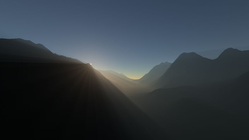
S. Hillaire / Production Ready Atmosphere Rendering

believe that rendering real-time sky and atmosphere using a path              [Hil16] H ILLAIRE, S ÉBASTIEN. “Physically Based Sky, Atmosphere and
tracer coupled with a denoiser is a promising research avenue.                  Cloud Rendering in Frostbite”. SIGGRAPH 2016 Course: Physically
                                                                                Based Shading in Theory and Practice. 2016 2, 4, 5, 8.
                                                                              [Hoo16] H OOBLER, NATHAN. “Fast, Flexible, Physically-Based Volumet-
Acknowledgments                                                                 ric Light Scattering”. Game Developers Conference. 2016 2, 9.
We would like to thank the anonymous reviewers for the useful                 [HW12] H OSEK, L UKAS and W ILKIE, A LEXANDER. “An Analytic
                                                                                Model for Full Spectral Sky-dome Radiance”. ACM Trans. Graph. 31.4
comments, as well as the entire rendering team at Epic Games
                                                                                (2012), 95:1–95:9 2.
for reviewing and proofreading the paper, especially Krzysztof
                                                                              [JMLH01] J ENSEN, H ENRIK WANN, M ARSCHNER, S TEPHEN R.,
Narkowicz, Charles de Rousiers, Graham Wihlidal and Dmitriy
                                                                                 L EVOY, M ARC, and H ANRAHAN, PAT. “A Practical Model for Subsur-
Dyomin. We would also like to thank Jean-Sebastien Guay, Jor-                   face Light Transport”. Proceedings of the ACM on Computer Graphics
dan Walker, Ryan Brucks, Sjoerd de Jong and Wiktor Öhman for                    and Interactive Techniques. 2001, 511–518 5.
providing level art and evaluating the technique. Lastly, we would            [Kar14] K ARIS, B RIAN. “High-Quality Temporal Supersampling”. Ad-
like to thank Stephen Hill for proofreading the paper.                          vances in Real-time Rendering in Games Part I, ACM SIGGRAPH 2014
                                                                                Courses. 2014, 10:1–10:1 9.
                                                                              [Kut13] K UTZ, P ETER. The Importance of Ozone. 2013. URL: http://
References                                                                      skyrenderer.blogspot.se/2013/05/the- importance-
[Bau19] BAUER, FABIAN. “Creating the Atmospheric World of Red Dead              of-ozone.html 3.
  Redemption 2: A Complete and Integrated Solution”. Advances in Real         [LdR14] L AGARDE, S EBASTIEN and de ROUSIERS, C HARLES. “Moving
  Time Rendering, ACM SIGGRAPH 2019 Courses. 2019 2, 9.                         Frostbite to PBR”. Physically Based Shading in Theory and Practice,
[BCR*10] BARAN, I LYA, C HEN, J IAWEN, R AGAN -K ELLEY, J ONATHAN,              ACM SIGGRAPH 2014 Courses. 2014 2.
  et al. “A Hierarchical Volumetric Shadow Algorithm for Single Scatter-      [NAS] NASA. Earth Fact Sheet. URL: https : / / nssdc . gsfc .
  ing”. ACM Trans. Graph. 29.6 (2010), 178:1–178:10 9.                          nasa.gov/planetary/factsheet/earthfact.html 3.
[BN08] B RUNETON, E RIC and N EYRET, FABRICE. “Precomputed Atmo-              [NDN96] N ISHITA, T OMOYUKI, D OBASHI, YOSHINORI, and NAKA -
  spheric Scattering”. Proceedings of Eurographics. 2008, 1079–1086 2–          MAE , E IHACHIRO . “Display of Clouds Taking into Account Multiple
  5, 7–9.                                                                       Anisotropic Scattering and Sky Light”. Proceedings of the ACM on Com-
[Bou08] B OUTHORS, A NTOINE. “Realistic rendering of clouds in real-            puter Graphics and Interactive Techniques. 1996, 379–386 2.
  time”. PhD thesis. Université Joseph Fourier, 2008. URL: http : / /         [NSJ] N OVÁK, JAN, S ELLE, A NDREW, and JAROSZ, W OJCIECH. “Resid-
  evasion . imag . fr / ~Antoine . Bouthors / research /                        ual Ratio Tracking for Estimating Attenuation in Participating Media”.
  phd/ 5.                                                                       ACM Trans. Graph. 33.6 (), 179:1–179:11 3.
[Bru17a] B RUNETON, E RIC. “A Qualitative and Quantitative Evaluation         [NSTN93] N ISHITA, T OMOYUKI, S IRAI, TAKAO, TADAMURA, K AT-
  of 8 Clear Sky Models”. IEEE Transactions on Visualization and Com-           SUMI , and NAKAMAE , E IHACHIRO . “Display of the Earth Taking into
  puter Graphics 23.12 (2017), 2641–2655 2, 3, 6.                               Account Atmospheric Scattering”. Proceedings of the ACM on Com-
[Bru17b] B RUNETON, E RIC. Precomputed Atmospheric Scattering. 2017.            puter Graphics and Interactive Techniques. 1993, 175–182 2.
   URL : https : / / github . com / ebruneton / precomputed _                 [ONe07] O’N EIL, S EAN. “Accurate Atmospheric Scattering”. GPU Gems
  atmospheric_scattering 2, 3, 8.                                               2. 2007 2.
[dCK17] De C ARPENTIER, G ILIAM and KOHEI, I SHIYAMA. “Decima En-             [PSS99] P REETHAM, A. J., S HIRLEY, P ETER, and S MITS, B RIAN. “A
  gine: Advances in Lighting and AA”. Advances in Real Time Rendering,          Practical Analytic Model for Daylight”. Proceedings of the ACM on
  ACM SIGGRAPH 2017 Courses. New York, NY, USA: ACM, 2017 2.                    Computer Graphics and Interactive Techniques. 1999, 91–100 2.
[EK10] E LEK, O SKAR and K MOCH, P ETR. “Real-time spectral scattering        [Val14] VALIENT, M ICHAL. “Making Killzone Shadow Fall Image Qual-
  in large-scale natural participating media”. Proceedings of the Spring        ity into the Next Generation”. Game Developers Conference. 2014 9.
  Conference on Computer Graphics (SCCG). 2010, 77–84 9.
                                                                              [Wen07] W ENZEL, C ARSTEN. “Real time atmospheric effects in game re-
[Ele09] E LEK, O SKAR. “Rendering Parametrizable Planetary Atmo-                visited”. Game Developers Conference. 2007 2.
   spheres with Multiple Scattering in Real-time”. CESCG (2009) 2, 3, 5.
                                                                              [Yan97] YANOVITSKIJ, E DGARD G. Light Scattering in Inhomogeneous
[EPI18] EPICGAMES. Unreal Engine 4.19: Screen percentage with                   Atmospheres. Springer-Verlag Berlin Heidelberg, 1997 5.
  temporal upsample. March 2018. URL: https : / / docs .
  unrealengine . com / en - US / Engine / Rendering /                         [Yus13] Y USOV, E GOR. “Outdoor Light Scattering”. Game Developers
  ScreenPercentage/index.html 9.                                                Conference. 2013 2, 5.
[FWKH17] F ONG, J ULIAN, W RENNINGE, M AGNUS, K ULLA, C HRISTO -              [ZYWK08] Z INKE, A RNO, Y UKSEL, C EM, W EBER, A NDREAS, and
  PHER , and H ABEL , R ALF . “Production Volume Rendering”. ACM SIG-           K EYSER, J OHN. “Dual Scattering Approximation for Fast Multiple Scat-
  GRAPH 2017 Courses. 2017 2, 3, 9.                                             tering in Hair”. ACM Trans. Graph. 27.3 (2008), 32:1–32:10 5, 6.
[GK99] G ARY E., T HOMAS and K NUT, S TAMNES. “Radiative transfer in
  the atmosphere and ocean”. Cambridge Univ. Press (1999) 3.
[GS16] G JOEL, M IKKEL and S VENDSEN, M IKKEL. “Low Complexity,
  High Fidelity - INSIDE Rendering”. Game Developers Conference.
  2016 9.
[HG13] H OLZSCHUCH, N ICOLAS and G ASCUEL, J EAN -D OMINIQUE.
  “Double- and Multiple-Scattering Effects in Translucent Materials”.
  IEEE Computer Graphics and Applications (2013), 66–76 5.
[Hil15] H ILLAIRE, S ÉBASTIEN. “Physically Based and Unified Volumet-
  ric Rendering in Frostbite”. Advances in Real Time Rendering, ACM
  SIGGRAPH 2015 Courses. 2015 6.

                                                                                                                                                    © 2020 The Author(s)
                                                                                  Computer Graphics Forum © 2020 The Eurographics Association and John Wiley & Sons Ltd.
You can also read